1
Syndromic surveillance using veterinary laboratory data: data pre-processing
and algorithm performance evaluation
Fernanda C. Dórea1; Beverly J. McEwen2, W Bruce McNab3; Crawford W. Revie1; Javier Sanchez1
1Department of Health Management, Atlantic Veterinary College, University of Prince Edward Island, Charlottetown, PE, C1A 4P3, Canada.
2Animal Health Laboratory, Ontario Veterinary College, University of Guelph, Guelph, ON, N1H 6R8, Canada
3Ontario Ministry of Agriculture Food and Rural Affairs, Guelph, ON, N1G 4Y2, Canada
Corresponding Author Fernanda Dórea
[email protected]. Department of Health Management, Atlantic Veterinary College, University of Prince Edward Island, Charlottetown, PE, C1A 4P3, Canada. Phone: +1(902)566-0969; Fax: +1(902)-620-5053.
Postal address:
2 Abstract
Diagnostic test orders to an animal laboratory were explored as a data source for monitoring trends in the incidence of clinical syndromes in cattle. Four years of real data and over 200 simulated outbreak signals were used to compare pre-processing methods that could remove temporal effects in the data, as well as temporal aberration detection algorithms that provided high sensitivity and specificity. Weekly differencing demonstrated solid performance in
removing day-of-week effects, even in series with low daily counts. For aberration detection, the results indicated that no single algorithm showed performance superior to all others across the range of outbreak scenarios simulated. Exponentially Weighted Moving Average charts and Holt-Winters exponential smoothing demonstrated complementary performance, with the latter offering an automated method to adjust to changes in the time series that will likely occur in the future. Shewhart charts provided lower sensitivity but earlier detection in some scenarios.
Cumulative Sum charts did not appear to add value to the system, however the poor performance of this algorithm was attributed to characteristics of the data monitored. These findings indicate that automated monitoring aimed at early detection of temporal aberrations will likely be most effective when a range of algorithms are implemented in parallel.
3 Introduction
During the last decade, increased awareness of the need to recognize the introduction of pathogens in a monitored population as early as possible has caused a shift in disease surveillance towards systems that can provide timely detection [1, 2]. Some monitoring has shifted to pre-diagnostic data, which are available early, but lack specificity for detection of particular diseases. These data can, however, be aggregated into syndromes, a practice which has led to an increase in the use of the terms "syndromic data", and "syndromic surveillance" [3, 2]. Disease outbreak detection is a process similar to that of statistical quality control used in manufacturing, where one or more streams of data are inspected prospectively for abnormalities [2]. For this reason, the use of classical quality control methods has been used extensively in public health monitoring [4, 5]. However, these types of control charts are based on the assumption that observations are independently drawn from pre-specified parametric
distributions, and therefore their performance is not optimal when applied to raw, unprocessed health data [6], which are typically subjected to the effect of factors other than disease burden. Some of these factors are predictable, such as day-of-week effects, seasonal patterns or global trends in the data [2]. These predictable effects can be modelled and removed from the data [7, 6, 8]. An alternative is to make use of data-driven statistical methods, such as the Holt-Winters exponential smoothing, which can efficiently account for temporal effects [9].
The use of real data is an essential step in the selection of algorithms and detection parameters because the characteristics of the baseline (such as temporal effects and noise) are likely to have a significant impact on the performance of the algorithms [10]. However, the limited amount of real data and lack of certainty concerning the consistent labelling of outbreaks in the data prevent a quantitative assessment of algorithm performance using standard measures such as sensitivity and specificity. These issues can be partially overcome through the use of simulated data which can include the controlled injection of outbreaks. Furthermore this approach has the advantage of allowing for the evaluation of algorithm performance over a wide range of outbreak scenarios [11].
A recent review [12] indicated that few systems have been developed for real- or near-real time monitoring of animal health data. Previous work by the authors [13] has addressed the possibility of using laboratory test requests as a data source for syndromic surveillance in aiming to monitor patterns of disease occurrence in cattle. In this paper these same data streams were used to evaluate different temporal aberration detection algorithms, with the aim of constructing a monitoring system that can operate in near-real time (i.e. on a daily and weekly basis). The points outlined above were addressed in an exploratory analysis designed to:
4
(ii) explore methods that combine these pre-processing steps with detection algorithms, with the data streams available and being aware of the importance of having a detection process
interpretable by the analysts;
(iii) identify the temporal aberration detection algorithms that can provide high sensitivity and specificity for this specific monitoring system.
A variety of algorithms and pre-processing methods were combined and their performance for near-real time outbreak detection assessed. Real data were used to select algorithms, while sensitivity and specificity were calculated based on simulated data which included the controlled injection of outbreaks.
Methods
All methods were implemented using the R environment (http://www.r-project.org/) [14].
Data source
Four years of historical data from the Animal Health Laboratory (AHL) at the University of Guelph in the province of Ontario, Canada, were available – from January 2008 to December 2011. The Animal Health Laboratory (AHL) is the primary laboratory of choice for veterinary practitioners submitting samples for diagnosis in food animals in the province of Ontario, Canada. The number of unique veterinary clients currently in the laboratory’s database (2008 to 2012) is 326. The laboratory receives around 65,000 case submissions per year, summing up to over 800,000 individual laboratory tests performed, of which around 10% refer to cattle
submissions, the species chosen as the pilot for syndromic surveillance implementation. A common standard for the classification of syndromes has not been developed in veterinary medicine. Classification was therefore established firstly upon manual review of three years of available data, and then creating rules of classification reviewed by a group of experts (a
5
and “others”. Diagnostics for specific agents assigned to an individual group due to higher volume (ii above) were: bovine leukaemia virus (BLV); bovine viral diarrhoea virus (BVD);
Mycobacterium paratuberculosis (Johnes disease) and Neospora caninum. Lastly, the groups
created to classify general tests (iii above) were: biochemical profile; other clinical pathology tests; toxicology tests; and nonspecific tests (those which could not be classified into any of the previous groups). All 16 syndromic groups were subjected to monitoring using the methods described below.
Individual health events were defined as one syndromic occurrence per herd, that is, multiple test requests associated with a veterinarian visit to the same herd on a given day, when classified into the same syndromic group, are counted as “one case”. In comparison to human medicine, this would mean that the herd is the individual patient (not each animal within a herd). Classification is first performed for each requested test. Once each test request is classified into a syndromic group, the data are collapsed by the unique herd identification for each day.Any cases in the database assigned to weekends were summed to the following Monday, and weekends were removed from the data. Only syndromic groups with a median greater than one case per day were monitored daily [13]. It was proposed that the remaining syndromes (7 of 17 in total) would be monitored on a weekly basis; these series are not discussed further in this paper. All the methods described in this paper were carried out for all the syndromic groups monitored daily. As documented in [13], the time series of daily cases for each of these groups showed very similar statistical properties: daily medians between 2 and 4, except for tests for diagnostic of mastitis and respiratory syndromes, which daily medians were 9 and 1, respectively; strong day of week effect; no global monotonic trends; and weak seasonal effects, especially for the syndromes with lower daily medians.
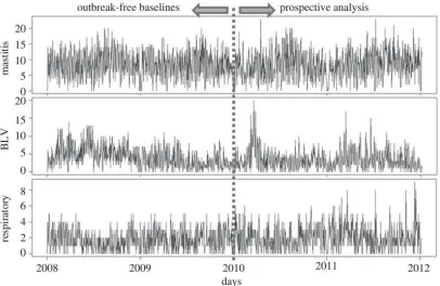
Methods and results will be illustrated using the daily counts of laboratory test requests for identification of Bovine Leukaemia Virus (BLV). Animals affected by bovine leukosis present a reduction in condition, diarrhoea, and tumours in several organs, which can sometimes be palpated through the skin, though more often only the unspecific signs are noted. Tests for BLV are often requested in animals showing a general reduction in condition. This series was chosen due to the statistical similarities to time series of other syndromic groups, while being the only times series showing evident presence of temporal aberrations (outbreak signals) documented in the historical data. Additionally, the counts of test requests for diagnostic of mastitis (inflamed udder in lactating cows) are used to illustrate the particular effect of working with time series with stronger seasonal effects; while the daily counts of laboratory submissions for diagnostic of respiratory syndromes is used to illustrate the particular challenges of working with time series with lower daily median. The three time series are shown in Figure 1.
6
Data from 2010 and 2011 were used to evaluate the performance of detection algorithms trained using those baselines.
Simulated data
In order to simulate the baseline (background behaviour) for each syndromic group the four years of data were fit to a Poisson regression model with variables to account for day-of-week and month, as previously documented [13]. The predicted value for each day of the year was set to be the mean of a Poisson distribution, and this distribution was sampled randomly to
determine the value for that day of a given year, for each of 100 simulated years.
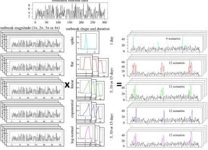
To simulate outbreak signals (temporal aberrations that are hypothesized to be documented in the data stream monitored in case of an outbreak in the population of interest) that also preserved the temporal effects from the original data, different outbreak signal magnitudes were simulated by multiplying the mean of the Poisson distributions that characterized each day of the baseline data by selected values. Magnitudes of 1, 2, 3 and 4 were used.
Outbreak signal shape (temporal progression), duration and spacing were then determined by overlaying a filter to these outbreak series, representing the fraction of the original magnified count which should be kept. For instance, a filter increasing linearly from 0 to 1 in 5 days
(explicitly: 0.2, 0.4, 0.6, 0.8 and 1), when superimposed to an outbreak signal series, would result in 20% of the counts in that series being input (added to the baseline) on the first day, 40% in the second, and so on, until the maximum outbreak signal magnitude would be reached in the last outbreak day. The process and resulting series are summarized in Figure 2. As can be seen in the figure, while the filters had monotonic shapes, the final outbreak signals included the random variation generated by the Poisson distribution. The temporal progression of an outbreak is difficult to predict in veterinary medicine, where the epidemiological unit is the herd rather than individual animals, because a large proportion of transmission is due to indirect contact between farms locally and also over large distances [16]. The same pathogen introduction can result in different temporal progressions in different areas as a result of spatial heterogeneity, as seen in the foot-and-mouth disease outbreak in the UK in 2001 [17] and the bluetongue outbreak in Europe in 2006 [18]. For this reason, several outbreak signal shapes previously proposed in the literature ([19, 20]) were simulated. These shapes were combined to generate the following filters:
a. Single spike outbreaks: A value of 1 is assigned to outbreak days, while all other days are assigned a value of zero.
b. Moving average (flat) outbreaks: Each outbreak signal is represented by a sequence of 5, 10 or 15 days (one to three weeks) with a filter value of 1 (outbreak days), separated by days of non-outbreak in which the filter value is zero.
7
d. Exponential increase: The filter value increases exponentially from 0 in the first day, to 1 in the last day. For the duration of 5 days this was achieved by assigning 1 to the last day, and dividing each day by 1.5 to obtain the value for the preceding day. For the durations of 10 and 15 days a value of 1.3 was used.
e. Log-normal (or sigmoidal) increase: The filter value increases following a lognormal curve from 0 in the first day, to 1 in the last day. The same values for the distribution are used for any outbreak signal length [lognormal(4, 0.3)], but the value corresponding to 5, 10 and 15 equally distributed percentiles from this distribution are used to assign the filter value for outbreaks with these respective durations.
Each filter was composed using one setting of outbreak signal shape and duration, repeated at least 200 times over the 100 simulated years, with a fixed number of non-outbreak days between them. The space between outbreak signals was determined after real data were used to choose the initial settings for the aberration detection algorithms, in order to ensure that outbreak signals were spaced far enough apart to prevent one outbreak from being included in the training data of the next. Each of these filters was then superimposed on the 4 different outbreak signal
magnitude series, generating a total of 52 outbreak signal scenarios to be evaluated independently by each detection algorithm.
Detection based on removal of temporal effects and use of control charts
Exploratory analysis of pre-processing methods
The retrospective analysis [13] showed that day-of-week (DOW) effects were the most important explainable effects in the data streams, and could be modelled using Poisson regression. Weekly cyclical effects can also be removed by differencing [6]. Both of the following alternatives were evaluated to pre-process data in order to remove the DOW effect:
i. Poisson regression modelling with day-of-week and month as predictors. The residuals of the model were saved into a new time series. This time series evolves daily by refitting the model to the baseline plus the current day, and calculating today’s residual.
ii. Five-day differencing. The differenced residuals (the residual at each time point t being the difference between the observed value at t and t-5) were saved as a new time series. Autocorrelation and normality in the series of residuals were assessed in order to evaluate whether pre-processing was able to transform the weekly- and daily-autocorrelated series into i.i.d. observations.
Control charts
The three most commonly used control charts in biosurveillance were compared in this paper: (1) Shewhart charts, appropriate for detecting single spikes in the data; (2) cumulative sums
8
weighted moving average (EWMA), appropriate for use in detecting gradual increases in the mean [5, 6].
The Shewhart chart evaluates a single observation. It is based on a simple calculation of the standardized difference between the current observation and the mean (Z-statistic); the mean and standard deviation being calculated based on a temporal window provided by the analyst
(baseline).
The CUSUM chart is obtained by:
where t is the current time point, Dt is the standardized difference between the current observed value and the expected value. The differences are accumulated daily (since at each time point t
the statistic incorporates the value at t-1) over the baseline, but reset to zero when the standardized value of the current difference, summed to the previous cumulative value, is negative. . The EWMA calculation includes all previous time points, with each observation’s weight reduced exponentially according to its age:
where is the smoothing parameter (>0) that determines the relative weight of current data to past data, It is the individual observation at time t and E0 is the starting value [21, 5].
The mean from values from the baseline are used as the expected value at each time point. Baseline windows of 10 to 260 days were evaluated for all control charts.
In order to avoid contamination of the baseline with gradually increasing outbreaks it is advised to leave a buffer, or guard-band gap, between the baseline and the current values being
evaluated [22, 23, 24]. Guard-band lengths of one and two weeks were considered for all algorithms investigated.
One-sided standardized detection limits (magnitude above the expected value) between 1.5 and 3.5 standard deviations were evaluated. Based on the standard deviations reported in the
literature for detection limits [25, 20, 26, 27], an arbitrary wide range of values was selected for the initial evaluation of this parameter.
For the EWMA chart, smoothing coefficients from 0.1 to 0.4 were evaluated based on values reported in the literature [28, 29, 27].
The three algorithms were applied to the residuals of the pre-processing steps.
Detection using Holt-Winters exponential smoothing
9
While regression models are based on the global behaviour of the time series, the Holt-Winters generalized exponential smoothing is a recursive forecasting method, capable of modifying forecasts in response to recent behaviour of the time series [9, 31]. The method is a
generalization of the exponentially weighted moving averages calculation. Besides a smoothing constant to attribute weight to mean calculated values over time (level), additional smoothing constants are introduced to account for trends and cyclic features in the data [9]. The time-series cycles are usually set to one year, so that the cyclical component reflects seasonal behaviour. However retrospective analysis of the time series presented in this paper [13] showed that Holt-Winters smoothing [31, 9] was able to reproduce DOW effects when the cycles were set to one week. The method suggested by Elbert and Burkom (2009) [9] was reproduced using 3 and 5-day-ahead predictions (n=3 or n=5), and establishing alarms based on confidence intervals for these predictions. Confidence intervals from 85% to 99% (which correspond to 1 to 2.6 standard deviations above the mean) were evaluated. Retrospective analysis showed that a long baseline yielded stabilization of the smoothing parameters in all time series tested when 2 years of data were used as training. Various baseline lengths were compared relative to detection performance. All time points in the chosen baseline length, up to n days before the current point were used to fit the model daily. Then the observed count of the current time point was compared to the confidence interval upper limit (detection limit) in order to decide whether a temporal aberration should be flagged [13].
Performance assessment
Two years of data (2010 and 2011) were used to qualitatively assess the performance of the detection algorithms (control charts and Holt-Winters). Detected alarms were plotted against the data in order to compare the results. This preliminary assessment aimed at reducing the range of settings to be evaluated quantitatively for each algorithm using simulated data.
The choice of values for baseline, guard-band and smoothing coefficient (EWMA) were
10
To optimize the detection thresholds, quantitative measures of sensitivity and specificity were calculated using simulated data. Sensitivity of outbreak detection was calculated as the
percentage of outbreaks detected from all outbreaks injected into the data. An outbreak was considered detected when at least one outbreak day generated an alarm. The number of days, during the same outbreak signal, for which each algorithm continued to generate an alarm was also recorded for each algorithm. Algorithms were also applied to the simulated baselines
directly, without the injection of any outbreaks, and all the days in which an alarm was generated in those time series were counted as false-positive alarms. Time to detection was recorded as the first outbreak day in which an alarm was generated, and therefore can only be evaluated when comparing the performance of algorithms in scenarios of the same outbreak duration. Sensitivity of outbreak detection were plotted against false positives in order to calculate the Area Under the Curve (AUC) for the resulting Receiver Operating Characteristic (ROC) curves.
Results
Preprocessing to remove the DOW effect
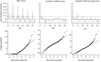
Autocorrelation function plots and normality Q-Q plots are shown in Figure 3 for the BLV series, for 2010 and 2011, to allow the two pre-processing methods to be evaluated. Neither method was able to remove the autocorrelations completely, but differencing resulted in smaller autocorrelations and smaller deviation from normality in all time series evaluated. Moreover, differencing retains the count data as discrete values. The Poisson regression had very limited applicability to series with low daily counts, cases in which model fitting was not satisfactory. Due to its ready applicability to time series with low as well as high daily medians, and the fact that it retains the discrete characteristic of the data, differencing was chosen as the
pre-processing method to be implemented in the system and evaluated using simulated data.
Qualitative evaluation of detection algorithms
Based on graphical analysis of the aberration detection results using real data, a baseline of 50 days (10 weeks) seemed to provide the best balance between capturing the behaviour of the data from the training time points and not allowing excessive influence of recent values. Longer baselines tended to reduce the influence of local temporal effects, resulting in excessive number of false alarms generated, for instance, at the beginning of seasonal increases for certain
syndromes. Shorter baselines gave local effects too much weight, allowing aberrations to contaminate the baseline, thereby increasing the mean and standard deviation of the baseline, resulting in a reduction of sensitivity.
11
days, the algorithms became insensitive to the aberrations during the last week of outbreak signal. The guard-band was therefore set to 10 days.
For the EWMA control charts, the number of alarms generated was higher when the smoothing parameter was greater, within the range tested. When evaluating graphically whether these alarms seemed to correspond to true aberrations, a smoothing parameter of 0.2 produced more consistent results across the different series evaluated and so this parameter value was adopted for the simulated data.
EWMA was more efficient than CUSUM in generating alarms when the series median was shifted from the mean for consecutive days, but no strong peak was observed. EWMA and Shewhart control charts appeared to exhibit complementary performance – aberration shapes missed by one algorithm were generally picked up by the other. CUSUM charts seldom improved overall system performance if the other two types of control chart had been implemented.
The performance of the Holt-Winters method was very similar with 3- and 5-day ahead predictions. Five-days ahead prediction was chosen because it provides a longer guard-band between the baseline and the observed data. Since this method is data-driven, using long baselines (2 years) did not cause the model to ignore local effects, but it did allow convergence of the smoothing parameters, eliminating the need to set an initial value. The method was set to read two years of data prior to the current time point. The use of longer baselines (up to 3 years) did not improve performance, but it would require longer computational time. The method did not appear to perform well in series characterised by low daily medians. In the case of the respiratory series, for instance, the Holt-Winters method generated 19 alarms over a period of 2 years, most of which seemed to be false alarms based on visual assessment (the control charts generated only 5-8 alarms for the same period).
Based on qualitative assessment alone, the range of detection limits to be evaluated using the simulated data could not be narrowed by more than half a unit for the control charts. It was therefore decided to evaluate 8 detection limits (in increments of 0.25) when carrying out the quantitative investigation: 2 to 3.75 for the Shewhart charts, 1.75 to 3.5 for CUSUM charts and for EWMA. For the Holt-Winters method confidence intervals greater or equal to 95% were investigated using simulated data.
Evaluation using simulated data
12
Longer outbreak lengths increased the sensitivity per outbreak, but reduced the number of days with alarms per outbreak in shapes with longer initial tails, as linear, exponential and lognormal. For these shapes a longer outbreak length also resulted in longer time to detection.
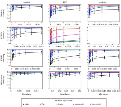
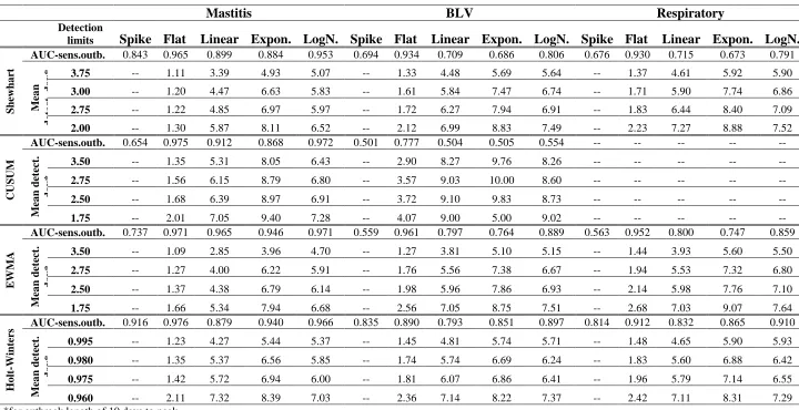
Receiver operating characteristics (ROC) curves for system sensitivities plotted against the number of false alarms are shown in Figure 4 for each of the four algorithms evaluated and the three syndromes. Lines in each panel show the median sensitivity for the five different outbreak shapes, along the eight detection limits tested. Error bars represent the 25% to 75% percentile of 12 scenarios, combining the four scenarios of outbreak magnitude (one to four times the
baseline) and the three scenarios of outbreak duration (one to three weeks) simulated. Area under the curve (AUC) for the plots are shown in Table 1, as well as median time to detection for the specific scenario of an outbreak of 10 days. A limited number of detection limits are shown in Table 1.
Starting at the first column of Figure 4 and Table 1, the results for the Mastitis simulated series, the sensitivity of detection of spikes and flat outbreaks was highest for the Holt-Winters method. EWMA charts showed low sensitivity for those, but the highest performance for all slow raising outbreak shapes (linear, exponential and lognormal). The lowest sensitivity within each
algorithm was for the detection of spikes, which is an artefact of the short duration of these outbreaks, compared to all other shapes. Similarly, the relatively high sensitivity for flat outbreaks can be interpreted as a result of the higher number of days with high counts in this scenario. Similarly, the performance for detection in lognormal shapes closely related to the flat outbreaks, being superior to linear and exponential increases. The CUSUM algorithm showed good performance in the Mastitis series, but its performance very quickly deteriorated for other series with smaller daily medians, as discussed below.
Median day of first signal for each outbreak, in the scenario of a 10 days to peak outbreak, are shown in Table 1 for a few key detection limits. Looking at the median day of detection for the flat and exponential outbreaks in the Mastitis series, it is possible to see, for instance, that even though the AUC is higher for the Holt-Winters (more outbreaks detected) when compared to the Shewhart chart, in case of detection the latter algorithm detects outbreaks earlier than the first. Moving to syndromes with lower daily counts, Figure 4 shows that the performance of all algorithms decreases as daily counts decrease. The problem is critical with the CUSUM
algorithm. Because this algorithm resets to zero if the difference in observed counts is lower than the expected counts, its application to a series with a large number of zero counts (Respiratory) resulted in no alarm being detected, true or false.
13
exponentially increasing outbreaks. Moving to even lower daily counts, as in the Respiratory series, the Holt-Winters method outperformed EWMA charts in all outbreak shapes but flat, the case for which both the EWMA charts and the Shewhart charts showed better performance than Holt-Winters.
The impact of the underlying baseline in the absence of outbreaks is also seen in the range of false positive values. The same detection limits generated a greater number of false alarms in the BLV series for all algorithms. Except for the BLV series, the number of false alarms generated in every scenario was smaller than 3% (1 false alarm in each 30 days of system operation). For the Holt-Winters method, a detection limit of 97.5% would always result in specificity greater than 97%, without loss of sensitivity compared to the lowest detection limits evaluated. For the EWMA charts a detection limit of 2 standard deviations represents the maximum attained specificity without starting to rapidly decrease sensitivity, but the behaviour should be evaluated individually for different syndromes. For the Shewhart chart such a cut-off seemed to rest on a detection limit of 2.25 standard deviations for the lower count series, but for the Mastitis series a limit of 2.5 would reduce false alarms with very little reduction in sensitivity.
Discussion
A recent review of veterinary syndromic surveillance initiatives [12] concluded that, due to the current lack of computerized clinical records, laboratory test requests represent the opportunistic data with the greatest potential for implementation of syndromic surveillance systems in
livestock medicine. In this paper we have evaluated two years of laboratory test request data, using the two preceding years as training data, and illustrated the potential of different
combinations of pre-processing methods and detection algorithms for the prospective analysis of these data where the primary aim is aberration detection.
A large number of studies have documented the use of public health data sources in syndromic surveillance, such as data from hospital emergency departments, physician office visits, over-the-counter medicine sales, etc. [32]. In veterinary health, however, the epidemiological unit for clinical data is usually the herd, rather than individual animals [12]. The number of
epidemiological units in a catchment area for individual data sources is therefore generally smaller than in public health monitoring, resulting in challenges around handling data with low daily counts, such as those described in this paper. It is hoped that the description of the steps taken to prepare these data and to select appropriate detection algorithms together with the results of this evaluation can guide the work of other analysts investigating the potential of syndromic data sources in animal health.
The data used for algorithm training had been previously evaluated retrospectively [13] and were found to have a strong day-of-week (DOW) effect. This effect prevented the direct use of
14
efficient method to remove daily autocorrelation; in line with a finding previously reported by Lotze et al (2008) [6]. Differencing has been recommended not only to remove DOW effects, but any cyclical patterns in addition to linear trends [6]. Five-day (weekly) differencing
demonstrated solid performance in removing the DOW effect, even in series with low daily counts, and preserved the data as count data (integers). Preserving the data as integers is important when using control-charts based on count data, and also in order to facilitate the analyst’s comprehension of both the observed and the pre-processed data series.
When pre-processed data were subjected to temporal aberration detection using control charts, EWMA performed better than CUSUM. EWMA’s superiority in detecting slow shifts in the process mean is expected from its documented use [6]. In the particular time series explored in this paper the general poor performance of the CUSUM was attributed to the low median values, when compared to traditional data streams used in public health. The injected outbreak signals were simulated to capture the random behaviour of the data, as opposed to being simulated as monotonic increases of a specific shape. Therefore, as seen in Figure 2, often the daily counts were close to zero even during outbreak days, as it is common for these time series. As a result, the CUSUM algorithm was often reset to zero, decreasing its performance. Shewhart charts showed complementary performance to EWMA charts, detecting single spikes that were missed by the first algorithm.
The use of control-charts in pre-processed data was compared to the direct application of the Holt-Winters exponential smoothing. Lotze et al. (2008) [6] have pointed out the effectiveness of the Holt-Winters method in capturing seasonality and weekly patterns, but highlighted the
potential difficulties in setting the smoothing parameters as well as the problems of one-day-ahead predictions. In this work the temporal cycles were set to weeks, and the availability of two years of training data allowed convergence of the smoothing parameters without the need to estimate initialization values. Moreover, the method worked well with predictions of up to 5 days ahead, which allows a guard-band to be kept between the training data and the actual
observations, avoiding contamination of the training data with undetected outbreaks [22, 23, 24]. Our findings confirm the conclusions of Burkom, et al., 2007 [31] who found, working in the context of human medicine, that the method outperformed ordinary regression, while remaining straight-forward to automate.
15
random effects were added by sampling from a Poisson distribution daily, rather than using model estimated values directly. Amplifying background data using multiplicative factors allowed the creation of outbreaks that also preserved the temporal effects observed in the background data.
Murphy and Burkom (2008) [24] pointed out the complexity of finding the best performance settings, when developing syndromic surveillance systems, if the shapes of outbreak signals to be detected are unknown. In this work the use of simulated data allowed evaluation of the
algorithms under several outbreak scenarios. Special care was given to outbreak spacing, in order to ensure that the baseline used by each algorithm to estimate detection limits was not
contaminated with previous outbreaks.
As the epidemiological unit in animal health is a herd, transmission by direct contact is not usually the main source of disease spread. Indirect contact between farms through the movement of people and vehicles is often a large component of disease spread [38]. The shape of the outbreak signal that will be registered in different health sources is hard to predict, and depends on whether the contacts, which often cover a large geographical area [16], will also be included in the catchment area of the data provider. The temporal progression of outbreaks of fast spreading diseases is often modelled as an exponential progression [39, 40], but data from documented outbreaks [18], and the result of models which explicitly take into account the changes in spread patterns due to spatial heterogeneity [41] more closely resemble linear increases. Linear increases may also be observed when an increase in the incidence of endemic diseases is registered, as opposed to the introduction of new diseases. Due to these uncertainties, all the outbreak signal shapes previously documented in simulation studies for development of syndromic monitoring were reproduced in this paper [11, 19, 36, 37].
Evaluation of outbreak detection performance was based on sensitivity and specificity, metrics traditionally used in epidemiology, combined using the AUC for a traditional ROC curve [42]. The training data used in this work to simulate background behaviour was previously analysed in order to remove aberrations and excess noise [13]. The number of false alarms when algorithms are implemented using real data is expected to be higher than that observed for simulated data. However, all the detection limits explored, generated less than 3% false alarm days (97% specificity) in the simulated data, which is the general fixed false-alarm rate suggested for biosurveillance system implementations [36]. Because the right tail of the ROC curves was flat in most graphs, it was possible to choose detection limits that provide even low rates of false alarms, with little loss of sensitivity.
16
recommended for the evaluation of prospective statistical surveillance [44], performance measures from the industrial literature were not used [43].
The results showed that no single algorithm should be expected to perform optimally across all scenarios. EWMA charts and Holt-Winters exponential smoothing complemented each other’s performance, the latter serving as a highly automated method to adjust to changes in the time series that can happen in the future, particularly in the context of an increase in the number of daily counts or seasonal effects. However, Shewhart charts showed earlier detection of signals in some scenarios, and therefore its role in the system cannot be overlooked. The CUSUM charts, however, would not add sensitivity value to the system.
Besides the difference in performance when encountering different outbreak signal shapes, the “no method fits all” problem also applied to the different time series evaluated. The performance of the same algorithm was different between two series with similar daily medians (results not shown). This was likely due to non-explainable effects in the background time series, such as noise and random temporal effects. Therefore, the choice of a detection limit which can provide a desired balance between sensitivity and false alarms would have to be made individually for each syndrome.
The use of these three methods in parallel – differencing+EWMA; differencing+Shewhart; and Holt-Winters exponential smoothing – ensures that algorithms with efficient performance in different outbreak scenarios are utilised. Methods to implement automated monitoring aimed at early detection of temporal aberrations occurrence using multiple algorithms in parallel will be evaluated in future steps of this work.
Acknowledgments
17 References
[1] Bravata DM, McDonald KM, Smith WM, Rydzak C, Szeto H, Buckeridge DL, et al. Systematic review: surveillance systems for early detection of bioterrorism-related diseases. Annals of Internal Medicine. 2004 Jun;140(11):910–922.
[2] Shmueli G, Burkom H. Statistical Challenges Facing Early Outbreak Detection in Biosurveillance. Technometrics. 2010;52:39–51.
[3] Centers for Disease Control and Prevention (CDC). Annotated Bibliography for Syndromic Surveillance; 2006. Acessed on June 17th, 2010. Available from: http://-www.cdc.gov/ncphi/disss/nndss/syndromic.htm.
[4] Benneyan JC. Statistical quality control methods in infection control and hospital epidemiology, part I: Introduction and basic theory. Infection Control and Hospital Epidemiology. 1998 Mar;19(3):194–214.
[5] Woodall WH. Use of Control Charts in Health-Care and Public-Health Surveillance. Journal of Quality Technology. 2006;38:2:89–104.
[6] Lotze T, Murphy S, Shmueli G. Implementation and Comparison of Preprocessing Methods for Biosurveillance Data. Advances in Disease Surveillance. 2008;6(1):1–20. ID: 1277. [7] Lotze T, Murphy SP, Shmueli G. Preparing Biosurveillance Data for Classic Monitoring. Advances in Disease Surveillance. 2007;2:55. ID: 1278.
[8] Yahav I, Shmueli G. Algorithm combination for improved performance in
biosurveillance systems. In: Proceedings of the 2nd NSF conference on Intelligence and security informatics: BioSurveillance. BioSurveillance’07. Berlin, Heidelberg: Springer-Verlag; 2007. p. 91–102. Available from: http://dl.acm.org/citation.cfm?id=1768376.1768388.
[9] Elbert Y, Burkom HS. Development and evaluation of a data-adaptive alerting algorithm for univariate temporal biosurveillance data. Statistics in Medicine. 2009 Nov;28(26):3226– 3248. Available from: http://dx.doi.org/10.1002/sim.3708.
[10] Buckeridge DL, Okhmatovskaia A, Tu S, O’Connor M, Nyulas C, Musen MA. Predicting outbreak detection in public health surveillance: quantitative analysis to enable evidence-based method selection. AMIA Annual Symposium Proceedings. 2008;1:76–80.
[11] Jackson ML, Baer A, Painter I, Duchin J. A simulation study comparing aberration detection algorithms for syndromic surveillance. BMC Med Inform Decis Mak. 2007;7:6. Available from: http://dx.doi.org/10.1186/1472-6947-7-6.
18
[13] Dórea FC, Revie CW, McEwen BJ, McNab WB, Kelton D, Sanchez J. Retrospective time series analysis of veterinary laboratory data preparing a historical baseline for cluster detection in syndromic surveillance. Preventive Veterinary Medicine. 2012;in press. Http://dx.doi.org/10.1016/j.prevetmed.2012.10.010.
[14] R Core Team. R: A Language and Environment for Statistical Computing. Vienna, Austria; 2012. ISBN 3-900051-07-0. Available from: http://www.R-project.org.
[15] Dórea FC, Muckle CA, Kelton D, McClure JT, McEwen B, McNab B, et al. Exploratory analysis of methods for automated classification of laboratory test orders into syndromic groups in veterinary medicine. PloSONE. 2013 Aug;In press(1-2). Available from: http://dx.doi.org/-10.1016/j.prevetmed.2011.05.004.
[16] Gibbens JC, Wilesmith JW, Sharpe CE, Mansley LM, Michalopoulou E, Ryan JBM, et al. Descriptive epidemiology of the 2001 foot-and-mouth disease epidemic in Great Britain: the first five months. Veterinary Record. 2001;149:729–743.
[17] Picado A, Guitian F, Pfeiffer D. Space-time interaction as an indicator of local spread during the 2001 FMD outbreak in the UK. Preventive Veterinary Medicine. 2007;79(1):3–19. [18] Santman-Berends IMGA, Stegeman JA, Vellema P, van Schaik G. Estimation of the reproduction ratio (R0) of bluetongue based on serological field data and comparison with other BTV transmission models. Preventive Veterinary Medicine. 2013;In press(0):–. Available from: http://www.sciencedirect.com/science/article/pii/S0167587712003662.
[19] Mandl KD, Reis B, Cassa C. Measuring outbreak-detection performance by using controlled feature set simulations. Morbidity and Mortality Weekly Report. 2004 Sep;53 Suppl:130–136.
[20] Hutwagner LC, Thompson WW, Seeman GM, Treadwell T. A simulation model for assessing aberration detection methods used in public health surveillance for systems with limited baselines. Statistics in Medicine. 2005 Feb;24(4):543–550. Available from: http://-dx.doi.org/10.1002/sim.2034.
[21] Stoumbos ZG, Reynolds MR, Ryan TP, Woodall WH. The State of Statistical Process Control as We Proceed into the 21st Century. Journal of the American Statistical Association. 2000;95(451):992–998.
[22] Burkom HS. Development, Adaptation, and Assessment of Alerting Algorithms for Biosurveillance. Johns Hopkins Apl Technical Digest. 2003;24(4):335–342.
19
[24] Murphy SP, Burkom H. Recombinant temporal aberration detection algorithms for enhanced biosurveillance. Journal of the American Medical Informatics Association. 2008;15(1):77–86. Available from: http://dx.doi.org/10.1197/jamia.M2587.
[25] Hutwagner LC, Maloney EK, Bean NH, Slutsker L, Martin SM. Using laboratory-based surveillance data for prevention: an algorithm for detecting Salmonella outbreaks. Emerging Infectious Diseases. 1997;3(3):395–400.
[26] Carpenter TE. Evaluation and extension of the cusum technique with an application to Salmonella surveillance. Journal of Veterinary Diagnostic and Investigation. 2002
May;14(3):211–218.
[27] Szarka JL 3rd, Gan L, Woodall WH. Comparison of the early aberration reporting system (EARS) W2 methods to an adaptive threshold method. Statistics in Medicine. 2011
Feb;30(5):489–504. Available from: http://dx.doi.org/10.1002/sim.3913.
[28] Nobre FF, Stroup DF. A monitoring system to detect changes in public health surveillance data. International Journal of Epidemiology. 1994 Apr;23(2):408–418. [29] Ngo L, Tager IB, Hadley D. Application of exponential smoothing for nosocomial infection surveillance. American Journal of Epidemiology. 1996 Mar;143(6):637–647. [30] Chatfield C. The Holt-Winters Forecasting Procedure. Applied Statistics. 1978;27(3):264–279.
[31] Burkom H, Murphy S, Shmueli G. Automated time series forecasting for biosurveillance. Statistics in Medicine. 2007 Sep;26(22):4202–4218. Available from: http://dx.doi.org/10.1002/-sim.2835.
[32] Hurt-Mullen KJ, Coberly J. Syndromic surveillance on the epidemiologist’s desktop: making sense of much data. Morbidity and Mortality Weekly Report. 2005 Aug;54 Suppl:141– 146.
[33] Buckeridge DL. Outbreak detection through automated surveillance: a review of the determinants of detection. Journal of Biomedical Informatics. 2007 Aug;40(4):370–379. Available from: http://dx.doi.org/10.1016/j.jbi.2006.09.003.
[34] Lotze TH, Shmueli G, Yahav I. In: Kass-Hout T, Zhang X, editors. Simulatin and
Evaluating Biosurveillance Datasets. Biosurveillance: Methods and Case Studies. United States: CRC Press; 2011. p. 23–51.
20
[36] Reis BY, Pagano M, Mandl KD. Using temporal context to improve biosurveillance. Proceedings of the National Academy of Sciences of the United States of America. 2003 Feb;100(4):1961–1965. Available from: http://dx.doi.org/10.1073/pnas.0335026100.
[37] Hutwagner L, Browne T, Seeman GM, Fleischauer AT. Comparing aberration detection methods with simulated data. Emerging Infectious Diseases. 2005 Feb;11(2):314–316.
[38] Dórea FC, Vieira AR, Hofacre C, Waldrip D, Cole DJ. Stochastic model of the potential spread of highly pathogenic avian influenza from an infected commercial broiler operation in Georgia. Avian Diseases. 2010 Mar;54(1 Suppl):713–719.
[39] Ferguson NM, Donnelly CA, Anderson RM. The Foot-and-Mouth Epidemic in Great Britain: Pattern of Spread and Impact of Interventions. Science. 2001;292(5519):1155–1160. Available from: http://dx.doi.org/10.1126/science.1061020.
[40] Keeling M, Woolhouse M, Shaw D, Matthews L, Chase-Topping M, Haydon D, et al. Dynamics of the 2001 UK foot and mouth epidemic: stochastic dispersal in a heterogeneous landscape. Science. 2001;294(5543):813–817.
[41] Kao RR. Landscape fragmentation and foot-and-mouth disease transmission. Veterinary Record. 2001;148:746–747.
[42] Wagner MM, Wallstrom G. In: Wagner MM, Moore AW, Aryel RM, editors. Methods for Algorithm Evaluation. Handbook of biosurveillance. UK: Academic Press; 2006. p. 301–310. [43] Fraker SE, Woodall WH, Mousavi S. Performance Metrics for Surveillance Schemes. Quality Engineering. 2008;20(4):451–464. Available from: http://www.tandfonline.com/doi/-abs/10.1080/08982110701810444.
[44] Sonesson C, Bock D. A Review and Discussion of Prospective Statistical Surveillance in Public Health. Journal of the Royal Statistical Society Series A (Statistics in Society).
21 Figure captions
Figure 1. Syndromic groups used to exemplify the times-series used in this work. Data from 2008 and 2009 have been analysed in order to remove temporal aberrations, constructing an outbreak-free baseline.
Figure 2. Synthetic outbreak simulation process. Data with no outbreaks were simulated reproducing the temporal effects in the baseline data. The same process was used to construct series that were for outbreak simulation, but counts were amplified up to 4 times. Filters of different shape and duration were then multiplied to these outbreak series. The resulting outbreaks were added to the baseline data.
Figure 3. Comparative analysis of the autocorrelation function and normality plots for the BLV series (years 2010 and 2011) before and after pre-processing.
22
23
24
25
26
Table 1. Performance evaluation of different detection algorithms. Area under the curve (for sensitivity of outbreak detection and percentage of simulated outbreak days with an alarm signal) was calculated using the median sensitivity for all scenarios of each outbreak shape (four outbreak magnitudes and three durations), plotted against false positive alarms, for the different detection limits shown. These curves are shown in Figure 4. The median detection days for the four outbreak magnitudes simulated for each outbreak shape, in the scenario of a 10 days outbreak length, are also shown.
Mastitis BLV Respiratory
Detection
limits Spike Flat Linear Expon. LogN. Spike Flat Linear Expon. LogN. Spike Flat Linear Expon. LogN.
Sh
ewha
rt
AUC-sens.outb. 0.843 0.965 0.899 0.884 0.953 0.694 0.934 0.709 0.686 0.806 0.676 0.930 0.715 0.673 0.791
M ea n det ec t. d ay
* 3.75 -- 1.11 3.39 4.93 5.07 -- 1.33 4.48 5.69 5.64 -- 1.37 4.61 5.92 5.90
3.00 -- 1.20 4.47 6.63 5.83 -- 1.61 5.84 7.47 6.74 -- 1.71 5.90 7.74 6.86
2.75 -- 1.22 4.85 6.97 5.97 -- 1.72 6.27 7.94 6.91 -- 1.83 6.44 8.40 7.09
2.00 -- 1.30 5.87 8.11 6.52 -- 2.12 6.99 8.83 7.49 -- 2.23 7.27 8.88 7.52
CUSU
M
AUC-sens.outb. 0.654 0.975 0.912 0.868 0.972 0.501 0.777 0.504 0.505 0.554 -- -- -- -- --
M ea n det ec t. da y *
3.50 -- 1.35 5.31 8.05 6.43 -- 2.90 8.27 9.76 8.26 -- -- -- -- --
2.75 -- 1.56 6.15 8.79 6.80 -- 3.57 9.03 10.00 8.60 -- -- -- -- --
2.50 -- 1.68 6.39 8.97 6.91 -- 3.72 9.10 9.83 8.73 -- -- -- -- --
1.75 -- 2.01 7.05 9.40 7.28 -- 4.07 9.00 5.00 9.02 -- -- -- -- --
E
W
M
A
AUC-sens.outb. 0.737 0.971 0.965 0.946 0.971 0.559 0.961 0.797 0.764 0.889 0.563 0.952 0.800 0.747 0.859
M ea n det ec t. da y *
3.50 -- 1.09 2.85 3.96 4.70 -- 1.27 3.81 5.10 5.15 -- 1.44 3.93 5.60 5.50
2.75 -- 1.27 4.00 6.22 5.91 -- 1.76 5.56 7.38 6.67 -- 1.94 5.53 7.32 6.80
2.50 -- 1.37 4.38 6.79 6.14 -- 1.98 5.96 7.86 6.93 -- 2.14 5.98 7.76 7.10
1.75 -- 1.66 5.34 7.94 6.68 -- 2.56 7.05 8.75 7.51 -- 2.68 7.03 9.07 7.64
H
o
lt
-Winte
rs
AUC-sens.outb. 0.916 0.976 0.879 0.940 0.966 0.835 0.890 0.793 0.851 0.897 0.814 0.912 0.832 0.865 0.910
M ea n det ec t. da y *
0.995 -- 1.23 4.27 5.44 5.37 -- 1.45 4.81 5.74 5.71 -- 1.48 4.65 5.90 5.93
0.980 -- 1.35 5.37 6.56 5.85 -- 1.74 5.74 6.69 6.24 -- 1.83 5.60 6.88 6.42
0.975 -- 1.42 5.72 6.94 6.00 -- 1.81 6.07 6.86 6.41 -- 1.96 5.79 7.14 6.55
0.960 -- 2.11 7.32 8.39 7.03 -- 2.36 7.14 8.22 7.37 -- 2.42 7.11 8.31 7.29 *for outbreak length of 10 days to peak.