Rochester Institute of Technology
RIT Scholar Works
Theses
Thesis/Dissertation Collections
4-15-1993
An Uncertainty analysis of a color tolerance
database
Mitchell Balonon-Rosen
Follow this and additional works at:
http://scholarworks.rit.edu/theses
This Thesis is brought to you for free and open access by the Thesis/Dissertation Collections at RIT Scholar Works. It has been accepted for inclusion
in Theses by an authorized administrator of RIT Scholar Works. For more information, please contact
.
Recommended Citation
AN UNCERTAINTY ANALYSIS OF A
COLOR TOLERANCE DATABASE
by
Mitchell Balonon-Rosen
B.S. Tufts University
(1983)
A thesis submitted in· par.tial fulfillment of the
requirement for the degree of Master of Science in
the Center for Imaging Science in the College of
Imaging Arts and Sciences of the Rochester
Institute of Technology
Mitchell Balonon-Rosen
Signature of the Author
_
Accepted by
Dana G. Marsh
~-2.
J!l2l
-J-COLLEGE OF IMAGING ARTS AND SCIENCES
ROCHESlER INSTITUIE OF lECHNOLOGY
ROCHESlER,
NEW
YORK
CERTIFICAlE OF APPROYAL
M.S. DEGREE THESIS
The M.S. Degree Thesis of Mitchell Balonon-Rosen
has been examined and approved by the thesis
committee as satisfactory for the thesis
requirement for the Master of Science degree
Dr. Roy Berns, Thesis Advisor
Dr. Mark Fairchild
THESIS RELEASE PERMISSION
ROCHESTER INSTITUTE OF TECHNOLOGY
COLLEGE OF IMAGING ARTS AND SCIENCES
AN UNCERTAINTY ANALYSIS OF A COLOR TOLERANCE DATABASE
I, Mitchell
Balonon-Rosen, hereby grant permission to the Wallace
Memorial Library of RJ.T. to reproduce my thesis in whole or in part.
Any reproduction will not be for commercial use or profit.
AN
UNCERTAINTY
ANALYSIS OF A
COLOR TOLERANCE DATABASE
by
Mitchell
Balonon-Rosen
Submitted
to
the
Center for
Imaging
Science
in
partial
fulfillment
of
the
requirements
for
the
Master
of
Science Degree
at
the
Rochester
Institute
of
Technology
ABSTRACT
Acknowledgments
It
is
with
great
appreciation
that
I
acknowledge
a
few
of
the
people
who
helped
me
and
stood
by
me
through
the
various
stages
of
this
work.
First,
I
would
like
to
single
out
my
thesis
advisor,
Dr.
Roy
Berns,
with
whom
it has been
a
source
of
pride
to
be
associated.
Dr.
Bern's
stewardship
of
the
Munsell
Color
Science
Laboratory
provides
a
comfortable
setting
for
serious
and
important
scholarship.
Since
my
departure
from
RIT,
Dr.
Berns
has
provided
me
with
a
level
of
long
distance
help
which
speaks
volumes
about
his
dedication
to
his
students'
successes.
The
completion
of
this
thesis
is
indeed
his
victory
as
it is
mine.
I
would
not
have
been
able
to
complete
this
thesis
had
it
not
been
for
the
help,
comradery
and
genuine
concern
provided
by
the
faculty,
staff
and
students
of
the
Munsell Laboratory.
In
particular
I
would
like
to
thank
Dr.
Mark
Fairchild,
my
teacher,
informal
advisor
and
a
member
of
my
thesis
committee,
and
fellow
students
Mr.
Mark
Gorzynski
and
Ms.
Lisa
Reniff,
also
a
member
of
my
thesis
committee.
Many
faculty,
staff
and
students
of
the
Center
for
Imaging
Science
were
instrumental
along
the
way
including
Dr.
Roger
Easton,
Ms.
Margaret
Evans,
Ms.
Susan
Chan,
Ms.
Colleen
Desimone
and
Mr.
Jeff
Loomis.
A
special
thanks
to the
50
members
of
the
R.I.T
community
who
volunteered
to
be
subjects
for
the
supplemental
experiments
carried
out
as
part
of
this
thesis.
I
would
like
to
acknowledge
Dr.
David
Alman
of
DuPont
Corporation for his
sponsorship
of
and
contributions
to
this
work,
Dr.
Jay
Thornton
and
Dr.
Richard Cottrell
of
Polaroid Corporation for
their
references,
meaningful
feedback
on
an
early
draft
and
for
being
a
grandfather
(his
words)
to
the
Munsell
Color
Science
students,
Mr.
Alan
Ames
of
Polaroid
for his
suggestion
that
I
use
cumulative
histograms
as
part
of
my
comparison
analysis,
and,
finally,
my
Uncle
Bill,
Dr.
William
Greenberg
of
Virginia
Polytechnic
Institute,
for
a
late-night
long-distance
explanation
of
eigen
vectors
("suppose
you
Dedication
December
6,
1992
This
thesis
is
dedicated
to
my
family:
to
my
parents,
Leonard
and
Adelaide
Rosen,
who
have
always
believed
one
hundred
percent
in
their
children,
to
Alma,
my
wife
and
friend,
who
has
supported
me
in
this
effort
for
years,
to
our
delightful
daughter
Marissa,
who's
entrance
on
the
scene
inspired
me
to
finish
this,
and
to
our
new
son
Peter,
born
14
days
ago,
may he
never
know
a
world
where
Daddy
is
Table
of
Contents
I.
Introduction
1
II.
Background
5
A. Uniform
Color-Spaces
and
Color-Difference
Formulae
5
B.
Overview
of
Color-Difference
Equations
7
C. Introduction
to
Phases
I
and
II
11
D. Probit Analysis
12
E. Differences Between Color Names in This
and
Previous
Papers
16
F. Phase
1
17
G. Phase
II
19
H. This Thesis
23
III.
Uncertainty
Analysis
26
A. Approach
26
B.
Supplemental Observations
26
C. Different Duration
of
Observer Session
31
D. Different Sample
AE*ab
Range
per
Vector
33
E.
Different Observer Population
34
F. Different
Vector
Orientations
35
G. Different Color Center Distance
From
Anchor
Pair
38
IV.
Median
Filtering
41
A.
Intra-Observer
Filtering
41
V.
Filtering
Effectiveness
and
Data
Pooling
74
A.
Filtering
Effectiveness
74
B. Data
Pooling
76
VI.
Color-Difference
Equation
Testing
81
A. Comparison
of
Filtered Data With
Color-Difference
Formulae
81
VB. Conclusions
88
Vffl. References
89
Appendix A: Tables
96
List
of
Tables
Table I:
Relating
currently
and
previously
used
color
names
16
Table II:
Vector
Directions Used
in Phase
1
17
Table HI:
Color
Centers
Used in Phase
1
17
Table IV:
Vector
Directions
Used in Phase
II
20
Table V:
Color
Centers
Used
in
Phase II
20
Table VI:
Color
Center Distance
from Anchor Pair
27
Table VII:
Anchor Pair
Measurements
and
Calculations
29
Table VIII: Results for Moderate Bluish Green Color Center....
30
Table IX:
Results for Light Bluish Green Color Center
31
Table X:
T-test
Comparison
of
Phase
II
and
Supplemental
Moderate Bluish Green
and
Light Bluish Green
Standard
Deviations
32
Table XI:
Paired
Samples T-test Comparison
of
Phase
II
and
Supplemental Light Bluish Green T50's
33
Table XII:
T-test
Comparison
of
Phase
I,
II
and
Supplemental
Moderate
Bluish
Green
Responses...
34
Table XIII:
Uncertainty
Indicators
for
Phase
I
and
II
Grouped
by
Vector Direction
37
Table XIV:
Uncertainty
Indicators
for
Phase
I
Grouped
by
Color Center
39
Table XV:
Uncertainty
Indicators
for Phase
II
Grouped
by
Color Center
39
Table XVI:
Frequency
Response for Noise
Free Observers
(Example
I)
43
Table XVII:
Frequency
Response for
Noisy
Observers
(Example
II)
45
Table XVIII:
Comparing
Phase
I
Unfiltered
to
Filtered
Frequency
Data
48
Table XIX:
Comparing
Phase
II Unfiltered
to
Filtered
Frequency
Data
57
Table XX:
T-test Comparison
of
Phase
I
and
II
Filtered
Moderate Bluish
Green Responses
76
Table XXI:
Filtering
results
summary:
77
Table XXII:
Statistics
on
Normalized
Color-Difference
Calculations
82
Table XXIII:
Kolmogorov-Smirnov Test
83
Table A-I:
Comparing
Current
Frequency
Data
to
Snyder's
96
Table
A-
II:
Comparing
Current
Frequency
Data
to
Reniffs
105
Table
A-
III:
Comparison
of
Various
Color-Difference
Formulae
List
of
Figures
Figure 1:
Anchor
and
Test-Pair
Configuration
2 9
Figure
2:
Phase I
and
Phase II Color Center
AE*ab
Distances
from Anchor Pair
3 8
Figure
3:
Average Stdev
as
Function
of
Color Center
Color-Distance from Anchor Pair for Combined Phase
I
and
II
4 0
Figure
4:
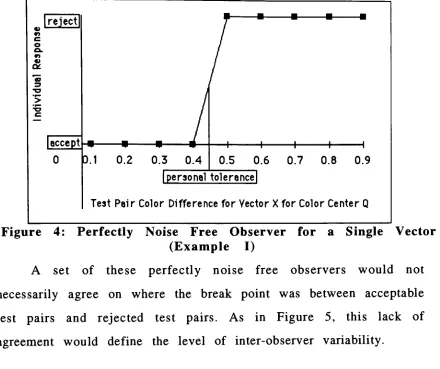
Perfectly
Noise Free Observer for
a
Single
Vector
(Example
I)
4
2
Figure
5:
Set
of
Noise Free
Observers
for
a
Single
Vector
(Example
I)
4 2
Figure
6:
Individual
Responding
as
if CIELAB
were
Non-Monotonic
Locally
(Example
II)
4
4
Figure 7:
Set
of
Observers
Responding
as
if CIELAB
were
Non-Monotonic
Locally
(Example
II)
4 4
Figure
8:
Median
Filter Examples
4 7
Figure 9:
Combined
Color-Difference
Cumulative
Histogram
8
4
Figure
10:
Comparison
of
Average Normalized
CMC(1:1)
and
BFD(1:1)
With Respect
to
Average Color Center L*..
8 5
Figure 11:
Comparison
of
Average
Normalized
CMC(1:1)
and
[image:11.520.81.469.46.368.2]I.
Introduction
A
multi-phase
research
project
has
been
underway
at
the
Munsell
Color
Science
Laboratory
to
create
a
database
of
experimentally
derived
human
color
difference
responses
for
a
large
subject
population
with
respect
to
a
wide
sampling
of
color-space.
Two
independent
studies,
Phase
I1-2
and
Phase
II3,
examined
a
total
of
nine
CIELAB7
color
directions in
the
vicinity
of
19
color
centers.
Although
the
studies
shared
similar
experimental
designs,
they
produced
very
different
confidence
statistics.
The
purpose
of
the
current
work
was
to
evaluate
differences
between
the
two
studies
and
determine
if pooling
the
data
was
appropriate.
Phases
I
and
II
took
advantage
of
an
experimental
method
which
enabled
a
quantitative
comparison
of
color-differences
throughout
color
space.
A
color-difference
standard
called
the
anchor
pair
was
used
for
these
comparisons.
It
consisted
of
two
near-neutral
painted
aluminum
samples,
differing
in
all
three
CIELAB
dimensions,
with
a
color-difference
magnitude
of
approximately
1
AE*ab
unit,
and
mounted
on
a
gray
background.
Color-differences
visually
matching
the
anchor
pair
were
dubbed
industrial-sized
because
of
their
importance
for
many
commercial
transactions.
The
anchor
pair
thus
measured
one
industrial-sized
color-difference
unit.
Test-pairs
were
of
similar
construction
to
the
anchor
pair.
Observers
were
asked
to
make
binary
forced
choice
determinations
as
to
whether
the
perceived
color-differences
of
test-pairs
were
greater
than
or
less
than
that
associated
with
the
anchor
The
inconsistency
between
currently
available
color-difference
scales
such
as
CIELAB
and
human
perceived
magnitudes,
particularly
in
the
realm
of
industrial-sized
color-differences,
was
the
main
motivation
behind
these
earlier
investigations.37"39
Snyder,1
Alman
et
al.,2Reniff,3
and
Berns
et
al.4have
produced
a
body
of
work
describing
the
background,
implementation
and
results
of
Phases
I
and
II.
They
have
justified
the
need
for
these
studies
and
have
thoroughly
explained
the
methodology
used
for
the
experimental
design
and
the
data
analysis.
In
order
to
put
the
current
work
in
proper
context,
the
aforementioned
papers
should
be
studied.
The
statistical
analysis
method
for
Phase
I
and
Phase
II
was
Probit
analysis.5Probit
was
designed
for
determining
population
tolerance
levels
for
quantal
experiments
where
observers
responded
normally
with
respect
to
a
stimulus
level
and
where
individual
observations
were
completely
independent.
The
stimulus
to
which
observers
reacted
in
Phases
I
and
II
was
test-pair
color-difference.
The
tolerance
level
sought
by
the
experiments
was
the
level
of
CIELAB
color-difference
corresponding
to
one
industrial-sized
color-difference
unit
at
various
points
in
color-space
and
in
particular
color-
space
orientations.
The
term
T50
was
used
in
these
studies
to
describe
the
median
tolerance
level
as
determined
by
Probit
analysis,
color
center
signified
locations
in
color-space
about
which
data
were
taken,
and
the
term
color
vector
was
used
to
designate
the
tri-valued
entity
comprising
the
resultant
T50
magnitude,
its
associated
color
center
and
its
color-space
orientation.
Phase
I
statistical
analysis
showed
an
observer
population
encouraging
statistics,
Phase II
results
were
cause
for
concern.
Only
47%
of
the
T50's
were
associated
with
high
confidence
measurements.3
The
current
project
was
mandated
the
responsibility
to
identify
the
differences
between Phases I
and
II
and
to
determine if
and
how
the
data
could
be
pooled.
Several
experiments
were
designed
to
test
theories
about
the
change
in
confidence
statistics.
These
experiments
helped
to
narrow
the
list
of
probable
primary
contributors.
The
most
likely
causes
for
the
decrease
in
statistical
confidence
were
identified
as
follows:
color-space
orientation
of
color-difference
test-pairs
and
the
color
distance
of
test-pair
colors
from
the
anchor
pair.
It
was
concluded
that
these
factors
resulted
in
making
Phase
II
a
more
difficult
task
for
observers.
A
median
filtering
technique
was
developed
for
use
on
the
raw
observer
responses.
The
effect
of
the
median
filter
was
to
reduce
within-observer
noise
so
that
the
Probit
analysis
could
properly
measure
between-observer
variation.
A
priori
knowledge
of
how
individuals
react
to
locally-increasing
color-differences
was
used
as
rationale
for
applying
the
filter.6
Phase
I
T50
metrics
were
changed
little
between
the
filtered
and
unfiltered
responses
where
maximum
magnitude
difference
was
0.03t
AE*ab
units.
91%
of
the
Phase II
filtered
T50's
were
within
0.10
AE*ab
units
of
the
unfiltered
values.
Filtered
Phase
I
data
showed
34+
of
its
45
color
vectors
passing
+
The
unfilteredPhase
I
andPhase
II
statisticsbeing
compared withthe
filtered
statisticsare
notthe
same asthose
reportedby
Snyder1,
Alman
et al.2and
Reniff3,
nor arethe
filtered
statistics
the
same asthose
reportedby
Berns
et al4.This is because
the
rawdata
was relogged
for
the
current study.For
further
explanation,
seethe
sections
Phase
I,
confidence
tests,
a
slight
decrease
from
35+
passing
prior
to
the
filtering.
Filtered Phase II
data
showed
an
increase
to
86+
from
56+
of
its
119
unfiltered
vectors.
The
filtered
results
were
compared
to
the
following
list
of
color-difference
formulae:
XYZ8
Euclidean
distance,
CIELAB7,
CIELUV7,
SVF9,
FMC210-11,
BFD(1:1)1213,
CMC(1:1)1415,
and
the
NBS
Unit
of
Color-Difference16-17.
CMC(1:1)
was
found
to
have
the
closest
II.
Background
A.
Uniform
Color-Spaces
and
Color-Difference
Formulae
In
1931
the
CIE
established
the
standard
observer
and
the
ability
to
calculate
trichromatic
responses.
This
provided
the
world
with
unambiguous
color
specification.
A
color
sample
described
by
XYZ
tristimulus
values
should
visually
match
another
sample
described
by
the
same
XYZ
tristimulus
values
under
identical
viewing
conditions.
The
ability
to
measure
colors
by
means
of
a
spectrophotometer
and
to
transform
measurements
to
XYZ
values
created
a
"universal
and
fundamental language
of
color."23The
1931
standard
observer
was
greatly
important
for
the
growth
of
color
science.
As
the
Handbook
of
Colorimetry23
pointed
out,
"Students
of
history
agree
that
man's
progress
was
slow
until
he
had
developed
a
language
that
enabled
him
to
impart
to
others
the
experience
that
he
had just
acquired."By
1934,
transformations
of
the
XYZ
system
were
being
developed
for
superior
correlation
between
calculated
distances
and
human
visual
perception.17Known
as
uniform
color
spaces
or
uniform
color
scales,
many
XYZ
transformations
have
been
offered
over
the
past
sixty
years.
Earliest
attempts
at
improving
the
non
uniform
nature
of
XYZ
space
concentrated
on
the
two-dimensional
projection
known
as
the
chromaticity
diagram.
MacAdam,
one
of
the
original
researchers
for
the
color
science
"Holy
Grail"
of
a
universal
uniform
color
space,
reminisced:25Analogous
to
Mercator
charts and otherkinds
of maps ofthe
worldthat
represent
perceptually
equal colordifferences
by
equaldistances
between
points
that
represent
equally
luminous
colors.
The
noticeability
of colordifferences
was notconsidered
-very
few
data
were available - whenthe
chromaticity
diagram
wasdevised
and
adopted.
However,
as soon asit
cameinto
use,
anomalies
wereencountered
in
interpreting
the
configurations ofpoints
onthe
diagram.
Inconsistencies
between
distances
and
perceivedmagnitudes
of colordifferences
were evident.The
analogy
withgeographical
maps wasquickly
noted andsuggestions
were madeto
changethe
representation
sothat
equaldistances
would representequally
noticeable
colordifferences.
The
hoped-for
chromaticity
diagram
withsuch
properties
came
to
be
called
"uniform".
The
searchfor
it
has
extended
over50
years and seems no nearerits
goalthan
atthe
beginning.
Much
ofthe
accumulated
evidenceindicates
that
the
goalis
unattainablethat
aflat
diagram
cannot represent equal colordifferences
by
equaldistances
any
morethan
aflat
map
ofthe
world can represent equalgeographical
distances
by
equaldistances
onthe
map.Without
a
uniform
color
space
it
was
necessary
to
perform
special
investigations
for
each
color
about
which
a
color
tolerance
was
to
be
specified.
MacAdam25
and
Billmeyer26
have described
the
use
of
"limit
standards"
which
are
chosen
as
representatives
of
acceptable
"extreme
variations."
Many
uniform
color
spaces
have
been
offered.
Hunter17
has
given
an
extensive
history
to
the
development
of
many
of
these
scales.
In
general,
the
scales
break down
into
three
categories:
those
deriving
from
the
work
of
Albert
Munsell:28-31
those
in
the
family
1940's
on
just-noticeable
differences33-34
(jnd's).
In
1976
the
CIE
recommended
that
the
color
community
use
either
of
two
color-difference
formulae,7-36
CIELAB
or
CIELUV.
CIELAB is
a
member
of
the
Munsell
family,
CIELUV
derives
from
MacAdam just-noticeable
difference
data.
As
these
and
their
derivations
have
become
the
most
dominant
uniform
color
spaces,
the
lack
of
best
fit
for
industrial-sized
color-differences
by
either
has
proven
troublesome.37"39
B.
Overview
of
Color-Difference
Equations
In
1969
Wright
wrote
"the
preference
for
one
[color-difference]
formula
over
another
is
likely
to
be
determined
by
its
practical
convenience
and
ease
of
application
rather
than
because
of
some
superior
visual
validity."40Over
the
years
and
between
industries,
these
criteria
have
had
inconsistent
interpretation.
For
example,
equations
once
thought
too
complicated
for
human
calculation
or
for
analog
circuitry
have
become
less
intimidating
as
computers
and
digital
circuitry
have
become
commonplace.
Yet,
simplicity
has
continued
to
be
a
driving
force.
Visual
factors
important
to
a
particular
niche
have
been
incorporated
into
formulae
only
to
find
indifference
from
the
color-difference
marketplace.
Historical
precedence,
as
well,
has
always
had
a
marked
influence
on
the
use
of
metrics.
"Practical
convenience"
is
often
defined
by
the
common
language,
regardless
of
its
appropriateness
to
the
problem
at
hand.
The
color-difference
formulae
compared
in
this
thesis
were
chosen
because
they
are
in
wide
use
today.
One
exception
is
the
NBS
was
derived
for
industrial-sized
color-differences.
Appendix
B
lists
the
formulae
for
these
equations.
The
NBS
unit
of
color-difference16-17also
known
as
the
Judd
col
or-difference
unit,
is
associated
with
the
Judd-Hunter
or
Modified
Judd
formula,
derived
by
Hunter
in
1942.
According
to
Hunter,
"differences
of
less
than
one
unit
are
usually
not
important
in
commercial
transactions."17
This
unit
was
based
on
Judd's
1939
formula,32
a
summary
of
dye
house
color-matching
investigations.
Hunter
transformed
the
1939
formula
to
his
"alpha-beta"rectangular
chromaticity
diagram
and
used
an
additional
10,000
observations
of
tile
samples.
The
formula
included
a
"gloss
factor,"considered
by
Hunter
as
late
as
1987
to
be
unique
among
uniform
color
spaces.17The
FMC-2
formula11
was
based
upon
the
FMC-1
metric.41The
earlier
formula
was
a
three-dimensional
fit
to
the
results
of
the
MacAdam
series
of
jnd
studies.
FMC-2
added
two
factors
to
better
conform
with
the
Simon-Goodwin
type
of
lightness
and
chromaticness
differences.42-43
The
first
factor
was
specifically
developed
for
textile
industry
use.
It
simulated
the
"swelling/
shrinking
behavior
of
Simon-Goodwin
chromaticness
differences."11
The
other
factor
was
developed
to
constrain
grays
to
conform
to
Simon-Goodwin
lightness
differences.
By
1976
it
was
recognized
that
as
many
as
20 different
color-difference
formulae
were
being
used
world
wide.7While
many
studies
were
made
comparing
the
various
available
formulae,
no
clear
winner
was
emerging.
At
the
time,
particularly
in
Europe,
ANLAB.
A disadvantage
to
the
formula
was
the
set
of
non-invertible
quintic
expressions
relating
fundamental
factors
to
the
CIE
XYZ
tristimulus
values.
In
order
to
estimate
these
factors,
table
lookups
and
interpolations
were
necessary.
A
simplification
using
cube-root
relationships
was
shown
to
deviate
from
the
original
insignificantly
and
grew
into
CIELAB.7
CIELUV7
was
derived
as
a
modification
to the
1964
CIE
U*V*W*
formula.46
Both
CIELUV
and
the
1964
formulas
had
associated
chromaticity
diagrams
with
desirable
properties
for
additive
systems.
Industries
that
worked
with
additive
colors,
such
as
color
television,
found
great
functionality
in
chromaticity
diagrams
which
preserved
a
colinear
relationship
between
the
chromaticities
of
any
two
colored
lights
and
the
chromaticity
of
their
weighted
combination.
The
position
of
the
resultant
chromaticity
was
directly
calculable
from
the
relative
radiance
levels.
No
such
diagram
was
available
for
CIELAB.
CIELAB
and
CIELUV
shared
a
common
lightness
component,
L*.
CMC(l:c),14
disclosed in
1984,
was
an
improvement
to the
JPC79
formula47-48
which,
in turn,
was
a
modification
of
ANLAB.52
JPC79
was
based
on
acceptability
results
obtained
in
one
study.12Under
the
direction
of
the
Society
of
Dyers
and
Colourists'
Colour
Measurement
Committee,
for
which
it
was
named,
CMC(l:c)
was
formed
to
remove
anomalies
introduced
in
lightness
differences
between
very
dark
colors
and
anomalies
introduced
in
hue
differences
between
near-neatral
colors.
The
CMC(l:c)
formula
also
added
the
T
and
'c'
attributes
which
allowed
application
specific
Reported
in
1986,
the
SVF9
color
space
was
an
attempt
to
"test
whether
it
was
possible
to
improve
the
quantitative
description
of
color-differences
by
introducing
a
few
physiological
assumptions
about
signal
processing
in
the
eye."In
particular,
three
aspects
of
contemporary
understanding
of
eye/brain
color
processing
were
addressed:
the
relationship
between
the
amount
of
light
incident
upon
the
three
cone
pigments
and
the
resultant
receptor
response;
the
relative
sensitivities
of
the
three
cone
types
and
their
saturation
characteristics;
and,
the
opponency
mechanism
for
chromatic
vision.
The
SVF
formula
was
a
modification
of
the
Munsell
Renotation
System.49
BFD(l:c)12-13
was
the
outcome
of
comparing
11
color-difference
formulae
to
a
combined
database
of
15
published
perceptibility
and
acceptability
data
sets.
A
total
of
132
color
centers
were
used.
While
CMC(l:c)
was
shown
to
perform
best,
systematic
errors
were
identified.
A
modification
of
CMC(l:c)
became
BFD(l:c).
BFD(lx)
was
designed
to
be
similar
in
structure
to
the
CMC(l:c)
formula
with
newly
derived
coefficients
and
an
additional
term
incorporated
to
correct
the
claimed
CMC(lx)
defect
of
always
orienting
discrimination
ellipsoids
toward
the
achromatic
axis
of
CIELAB.
Of
the
above
formulae,
FMC-2
and
CMC(l:c)
do
not
always
calculate
the
same
color-difference
between
two
colors
when
the
assigned
the
role
of
standard
is
changed.
This
has
often
been
considered
an
undesirable
characteristic.
The
use
of
weighted
CIELAB
AE*ab
components,
enjoyed
by
both
CMC(l:c)
and
BFD(l:c),
is
C.
Introduction
to
Phases
I
and
II
"It
may
be
noted
that
all
color-difference
formulas
are
designed
to
provide
results
that
describe
or
fit
well
one
or
another
body
of
visual
data (but
not
more
than
one,
since
these
data
sets
are
not
consistent
with
one
another)."35Here
Billmeyer
and
Saltzman
make
reference
to
one
of
the
most
important
motivations
for
this
study
and
its
predecessors.
Uniform
color
spaces
were
derived
from
and
fit best
one
or
another
data
set.
As described
above,
most
color-difference
formulae
can
be
traced
back
to
one
of
three
data
sets.
It
follows
that
each
formula
is
best
suited
to
deliver
psychophysical^
accurate
color-difference
magnitudes
for
differences
which
are
similar
to
those
comprising
its
associated
data
set.
While
the
Judd
family
of
color
spaces
actually
did
derive
from
commercially
important
color-differences,
Munsell-based
formulae
and
MacAdam
just-noticeable
difference
color
spaces
did
not.
Munsell
spacing
is
very
large
with
respect
to
industrial-sized
color-differences.
Just-noticeable
differences
are
very
small
with
respect
to
industrial-sized
color-differences.
Recall
that
the
two
current
CIE
recommended
color-difference
formulae,
CIELAB
and
CIELUV,
derive
respectively
from
Munsell
and
MacAdam
jnd
spaces.
Phases
I
and
II
were
designed
to
gather
data
about
human
perception
of
industrial- sized
color-differences.
In
1989,
Alman
et
al.2reported
the
results
of
Snyder's1
color
tolerance
experiment.
This
experiment
has
been
referred
to
as
Phase
industrial-sized
color-difference,
was
chosen
as
the
anchor
pair.
Using
a
psychophysical
technique
of
paired
comparison,
test-pairs
were
compared
to
the
anchor
pair.
Fifty
color-normal
observers
volunteered
for
the
experimental
task.
Observers
viewed
a
randomized
set
of
test-pairs.
For
each
pair,
observers
were
given
the
forced
choice
between
designating
"pass",
if
the
perceived
magnitude
of
the
test-pair
color-difference
were
smaller
than
that
of
the
anchor
pair,
or
"fail",
if
otherwise.
The
two
painted
colors
used
to
create
the
test-pairs
were
carefully
chosen
so
that
they
were
orientated
in
one
of
five
color
directions.
For
Phase
I,
each
vector
was
associated
with
one
of
nine
distinct
color
centers.
The
Reniff3
study,
referred
to
as
Phase
II,
was
a
follow-up
of
the
earlier
Phase
I
work.
Again,
fifty
color-normal
volunteers
were
assembled.
Conceptually,
the
task
was
identical
to
Phase
I.
Observers
were
asked
to
accept
a
test-pair
if
its
color-difference
were
smaller
than
the
anchor
pair's
and
reject
it
if
its
color-difference
were
larger.
The
anchor
pair
was
the
same
standard
as
had
been
used
in
Phase
I.
Test-pair
physical
dimensions
were
likewise
identical
to
those
used
in
Phase
I.
Phase
II
vectors
were
oriented
in
one
of
seven
color
directions
and
associated
with
one
of
17
color
centers.
D.
Probit
Analysis
Observer
rejection
rates
were
processed
through
Probit
which
would
have
been
perceptually
equivalent
to
the
anchor
pair's
color-difference.
Referred
to
as
the
T50,
this
equivalent
CIELAB
color-difference
is
an
estimate
of
that
which
would
have
been
rejected
by
exactly 50%
of
the
population.
The
SAS54
computer
statistical
package
was
used
to
perform
the
Probit
analysis.
In
addition
to
the
T50
values
the
SAS
program
calculated
for
each
vector
an
associated
a
(standard
deviation),
ax2value
and
a
%2confidence
value.
This
x2confidence
value
indicated
the
probability
that
the
true
x2were
greater
than
the
reported
%2.
Each T50
value
also
had
an
associated
fiducial limit
range,
similar
to
a
confidence
interval.
Probit
was
designed
for
situations
where
it
would
be
impractical
or
impossible
to
implement
a
method
of
limits
analysis.
An
experiment
utilizing
Probit
analysis
must
meet
the
following
criteria:
discrete
stimulus
levels
must
be
presented
to
subjects;
the
subject
population
should
respond
in
a
normal
manner
to
the
stimulus;
and,
each
individual
response
must
be
completely
independent
of
all
others.
The
Phase
I
and
Phase
II
experiments
were
quantal
in
nature.
Subjects
were
asked
to
respond
to
discrete
color-difference
magnitudes
associated
with
prefabricated
test-pairs.
The
Probit
criterion
that
the
population
respond
in
a
normal
manner
was
tested
within
the
analysis
for
each
T50
and
the
goodness-of-fit
was
quantified
in
the
%2probability
term.
As
described
above,
Probit
analysis
would
have
been
applied
inappropriatly
had
there
been
a
dependence
between
responses.
entertain
the
possibility
that
there
exist
experiments
which
could
reuse
subjects
to
receive
multiple
stimulus
levels.
It
assumed
that
this
would
automatically
violate
the
"independence"criterion.
This
conservative
stance
prevented
any
situation
where
a
residual
effect
from
earlier
observations
influenced
later
responses,
potentially
skewing
results.
"For
the
method
to
be
satisfactory,
there
must
be
no
cumulative
effect
of
doses
already
given,
either
as
lowering
or
as
increasing
the
resistance
of
the
subject,
a
condition
which
severely
limits
its
applicability."5Jameson
and
Hurvich
have
noted
that
perceived
color
is
"systematically
dependent
on
both
preceding
stimulation
and
on
simultaneous
stimulation
of
the
remainder
of
the
visual
field."73
However,
the
experiment
on
which
Jameson
and
Hurvich
based
their
claim
was
primarily
concerned
with
the
latter
phenomenon
followed
by
postulation
that
preceding
stimulus
would
have
similar
effect.
Conversely,
Berns
reported
general
acceptance
in
the
color
science
community
that
it
would
be
unreasonable
to
"expect
hysteresis
or
build-up
for
color-difference" observations.55
T50
represented
that
level
of
stimulus
which
would
have
caused
positive
response
in
50%
of
the
population.
The
stimulus
for
these
studies
was
color-difference.
The
T50,
in
CIELAB
AE*ab
units,
was
used
to
determine
the
population
match
to
the
visual
appearance
of
the
anchor
pair's
color-difference
for
each
color
direction
at
each
color
center.
The
x2was
representative
of
the
deviation
of
observer
responses
from
the
normality
assumption.
The
X2
and
the
number
of
degrees
of
freedom
were
used
to
lookup
a
x2distribution"6,
x2probability
terms
of
greater
than
5%
showed
good
model
fit.
The
standard
deviation
was
associated
with
the
cumulative
normal
curve
to
which
the
actual
responses
were
fit.
Fiducial
limits
delimited
the
error
range
about
the
T50
for
a
given
level
of
probability.
Fiducial
limits
were
calculated
using
a
95%
confidence
level.
The
Probit
procedure
used
an
iterative
process
to
estimate
p
and
a
such
that
f(x)
=X
1
(1)62
y2n
a
where
x
is
the
stimulus
level
and
f(x)
is
the
population
fractional
response.
For
the
purposes
of
these
studies,
reported
T50's
were
the
estimated
p's,
reported
standard
deviations
were
the
estimated
a's,
and
the
x2and
x2probability
terms
indicated
how
closely
the
estimated
curves
fit
the
raw
data.
The
stimulus,
x,
was
measured
in
AE*ab
units.
Equation
(1)
can
be
rewritten
as
follows:
AE*ab
rf(AE*ab)
=L_
(2)
ylnc
E.
Differences
Between
Color
Names
in
This
and
Previous
Papers
Snyder1
and
Alman
et
al.,2in reporting Phase
I,
and
Reniff,3
in
reporting
Phase
II,
used
color
names
convenient
for
the
purposes
of
their
investigations,
but
not
based
on
any
standard
naming
conventions.
Berns
et
al.4derived
the
ISCC-NBS
color
names22and
ISCC-NBS
colornames
are
defined
for
illuminant C
andthe
1931
standard
observer.
CIELAB
was used as achromatic-adaption
transformation
to
convert
the
experimental
color-center
values
based
onilluminant
D65
and
the
1964
supplementary
standard
observer
to
the
required
illuminant
andobserver.
Although CIELAB
is
wellknown
to
be
not anaccurate
adaptation
transformation,
its
useseemed
reasonable
for
the
purpose
ofmerely
assigning
colornames.
Table
I:
Relating
currently
names
and
previously
used
color
ISCC-NBS
color name
Previouslv
used name
Oriainal
Phase
Phase
1
Moderate blue
Blue
Moderate
greenish
blue
Cyan
Phase
1
Medium gray
Gray
Phase
1
Moderate bluish
green
Green
Phase
1
Light brown
Orange
Phase
1
Grayish
purple
Purple
Phase
1
Dark
reddish orange
Red
Phase
1
Moderate
yellow
Yellow
Phase 1
Grayish
yellow green
Yellow/Green
Phase
1
Black
Black
Phase
II
Light bluish
green
Blue/Green
Phase II
Moderate
reddish
brown
Brown
Phase
II
Dark bluish
green
Green/Blue
Phase II
Brilliant
greenish
blue
Light Blue
Phase II
Very
dark
red
Maroon
Phase
II
Moderate
purplish
pink
Pink
Phase
II
Dark blue
Violet
Phase II
Light gray
White
Phase
II
Strong
orange yellow
Yellow/Orange
Phase
II
Where
ever
possible
in
this
paper,
the
ISCC-NBS
names
have
been
used.
Table
I
displays
the
previously
used
and
current
names
F.
Phase
I
The
vector
directions
used
in
Phase
I
appear
in
Table
II.
Descriptions
of
the
color
centers
and
the
anchor
pair,
appear
in Table
III.
Five
of
the
nine
color
centers
used
corresponded
to
the
CIE
recommended
centers
for
coordinated
research.39Those
which
fulfill
this
criteria
contain
'yes'in
the
second
column.
Table
II:
Vector
Directions
Used
in
Phase
I
Vector Direction Name
CIELAB
orientation
A
to
+L*B
to
+a*C
to
+b*D
to
+a*,+b*E
to
+a*,-b*Table
III:
Color
Centers
Used
in
Phase
I
Color Center
CIE
recomd.
L* a* b*
AE*ab
from
Anchor
Anchor
49.21
0.045
5.275
-Moderate
yellow
yes
77.2
2.0
36.0
41.6
Grayish
yellow green
64.6
-9.913.2
20.0
Moderate bluish
green
yes
55.0
-27.72.0
28.5
Moderate blue
yes
34.2
-1 .0 -28.036.5
Grayish
purple
45.6
11.4
12.6
21.5
Moderate
greenish
blue
49.1
-16.2 -11
.523.4
Dark
redish orange
yes
42.8
34.7
22.8
39.4
Light
brown
61.2
13.2
20.0
23.1
Medium
Gray
yes
58.2
-0.30.8
10.0
A
high
degree
of
confidence
that
the
Phase
I
observer
population
was
consistent
and
had
a
distribution
equivalent
to
a
cumulative
normal
response
was
revealed
through
the
Probit
analysis.
Only
eight
of
the
45
Phase
I
vectors
revealed
statistically
Reported
statistics
in
Snyder1
and
Alman
et
al.2were
based
on
Snyder's
experimentally
derived
data.
The
visual
task
was
for
observers
to
accept
or
reject
test-pairs
based
on
comparison
of
the
color-difference
magnitude
to
that
of
the
anchor
pair.
When
an
observer
indicated
that
a
test-pair
passed,
Snyder
handwrote
a
check
mark
(
v
)
on
a
preprinted
form
next
to
a
number
representing
the
accepted
test-pair.
When
an
observer
indicated
that
a
test-pair
failed,
Snyder handwrote
an
'ex'mark
( X )
instead
at
the
same
place
on
the
response
form.
The
current
research
necessitated
a
return
to
the
original
response
forms.
Handwritten
check
marks
and
ex
marks
can
be
extremely
hard
to
distinguish.
The
use
of
the
two
marks
to
represent
opposite
responses
was
a
very
poor
choice.
After
examining
the
results
of
Snyder's
population
totals,
317
response
frequencies
from
50
observers,
and
comparing
them
with
the
current
totals,
tallied
from
photocopies
of
the
original
50
forms,
it
was
clear
that
certain
ambiguous
marks
had
been
interpreted
previously
as
denoting
acceptance
or
rejection
and
currently
as
the
opposite.
There
was
no
possibility
to
tell
which
marks
were
the
ones
with
which
the
researchers
had
disagreed.
It
was
only
possible
to
tell
which
test-pairs
were
affected
by
comparing
the
total
number
of
rejections
tabulated.
Table
A-I
presents
the
differences
between
Snyder's
totals
and
the
ones
used
for
the
current
research.
Note
that
Table
A-I
shows
only
unfiltered
responses.
Results
of
filtered
response
values
based
upon
the
current
data
were
reported
by
Berns
et
al.4Bluish
Green
showed
a
very
large
difference.
This
has
been
determined
to
be due
to
a
typographical
error
on
Snyder's behalf.
77
of
the
317
test-pairs
used
in
Phase I
showed
a
discrepancy
between
the
current
and
Snyder
tallies.
20%
of
the
45
Phase
I
T50
values
were
derived
using
none
of
the
discrepant
test-pairs.
The
other
36
T50's
were
derived
using
at
least
one
of
the
77
unagreed
upon
response
frequencies.
Ignoring
the
suspected
typographical
error
demonstrated
by
Moderate
Bluish
Green
vector
B,
the
largest
frequency
discrepancy
had
of
magnitude
of
3
observer
responses
and
no
T50
value
changed
by
more
than
.03CIELAB
AE*ab
units.
These
differences
are
considered
minuscule
and
are
certainly
within
experimental
error.
Only
the
current
data
were
used
for
the
present
research.
G.
Phase
II
The
exceptional
Phase
I
results
were
used
to
justify
an
optimistic,
ambitious
effort
for
Phase
II
utilizing
the
same
experimental
approach.
Four
new
vector
directions
were
added
to
each
of
the
original
color
centers.
Unlike
any
Phase
I
vectors,
these
new
directions
varied
simultaneously
in
all
three
dimensions
of
L*,
a*and
b*.
Also,
ten
new
color
centers
were
investigated.
These
centers
were
generally
much
further
in
AE*ab
distance
from
the
neutral
anchor
than
were
the
Phase
I
centers.
For
these
new
color
centers,
seven
vector
directions
were
tested.
Included
were
the
four
new
vector
directions
and
three
of
the
original
directions.
The
seven
Table
IV:
Vector
Directions
Used
in
Phase
II
Vector Direction Name
CIELAB
orientation
Also
in
Phase
1
A
to
+L*yes
B
to
+a*yes
C
to
+b*yes
F
-LVaVb*to
+L\+a*.+b*G
-L*,+a*,-b*to
+L*,-a*,+b*H
-L\+a*,+b*to
+LVa*.-b*1
-L*,-a*,+b*to
+L*,+a*,-b*Table
V:
Color
Centers
Usee
in
Phase
II
Color Center
CIE
recomd.
L* a* b*
AE*ab
from
Anchor
Also in
Phase I
Anchor
49.21
0.045
5.275
-yes
Moderate
yellow
yes
77.2
2.0
36.0
41.6
yes
Grayish
yellow green
64.6
-9.913.2
20.0
yes
Moderate bluish
green
yes
55.0
-27.72.0
28.5
yes
Moderate blue
yes
34.2
-1 .0 -28.036.5
yes
Grayish
purple
45.6
11.4
-12.621.5
yes
Moderate
greenish
blue
49.1
-16.2 -11
.523.4
yes
Dark
redish orange
yes
42.8
34.7
22.8
39.4
yes
Light brown
61.2
13.2
20.0
23.1
yes
Medium
Gray
yes
58.2
-0.30.8
10.0
yes
Light
Gray
83.0
0.4
0.1
34.2
Strong
orange yellow
75.0
17.2
78.4
79.4
Light bluish
green
68.2
-30.2 -5.437.3
Brilliant
greenish
blue
59.4
-13.1 -26.135.5
Moderate
purplish
pink
67.6
31.2
-0.236.6
Dark
bluish<