FRANCESCA ARRIGO†, DESMOND J. HIGHAM†, AND VANNI NOFERINI‡ Abstract. The combinatorics of walks on a graph is a key topic in network science. Here we study a special class of walks on directed graphs. We combine two features that have previously been considered in isolation. We consider alternating walks, which form the basis of algorithms for hub/authority detection and for discovering directed bipartite substructure. Within this class, we restrict to non-backtracking walks, since this constraint has been seen to offer advantages in related contexts. We derive a recursive formula for counting the total number of non-backtracking alternating walks of a given length, leading to an expression for any associated power series expansion. We discuss computational issues for the widely used cases of resolvent and exponential series, showing that non-backtracking can be incorporated at very little extra cost. We also derive an appropriate asymptotic limit which gives a parameter-free, spectral analogue. We perform tests on an artificial data set in order to quantify the advantages of the new methodology. We also show that the removal of backtracking allows us to identify larger bipartite subgraphs within an anatomical connectivity network from neuroscience.
Key words. bipartivity, centrality, directed graph, generating function, matrix polynomial, network
AMS subject classifications. 65F60, 68R10
1. Motivation. The notion of a walk around a graph is both natural and useful. However, in some settings, walks that backtrack—setting out from a node and then returning to it on the next step—are best avoided. The idea of restricting attention tonon-backtracking walks has been suggested and analysed in a wide range of fields, including spectral graph theory [2,21,22], number theory [35], discrete mathematics [11, 31], stochastic analysis [1], applied linear algebra [32] and computer science [30,
36]. In particular, in the area of network science non-backtracking walks have been shown to form the basis of effective algorithms for finding communities [23, 25] and assigning centrality values to nodes [6, 17, 26, 28]. From [5, 6, 17, 25, 26, 30] we know that advantages of the non-backtracking approach include
• low computational cost—comparable with, or less than, the backtracking counterparts,
• avoidance of localization (where most of a measure is assigned to a finite subset of the nodes),
• greater flexibility—a larger radius of convergence in the associated power series, which leads to a wider choice for the corresponding method parameter. In this work, we extend the non-backtracking idea to the case ofalternating walks
on directed graphs. This allows us to develop new theoretical results that lead to novel extensions of existing algorithms.
The work is organised as follows. In Section 2 we set up the basic notation and recall the idea of an alternating walk. In Subsections 3.1 and 3.2 we describe how alternating walks have been used to define algorithms for discovering bipartiv-ity and assigning nodal centralbipartiv-ity. The new contributions begin in Section 4, where
∗Submitted to the editors DATE.
Funding:DJH and FA are supported by grant EP/M00158X/1 from the EPSRC/RCUK Digital Economy Programme.
†Department of Mathematics and Statistics, University of Strathclyde, Glasgow, UK
([email protected],[email protected]).
‡Department of Mathematical Sciences, University of Essex, Wivenhoe Park, CO4 3SQ,
Colch-ester, UK ([email protected]).
we consider non-backtracking analogues of alternating walks. After formalizing the definitions, we derive in Theorem 4.1new, explicit recurrences that count the total number of non-backtracking alternating walks of any length. This gives a natural extension of the two and three term recurrences that arise in the non-alternating case. Using this result, we derive in Theorem 4.3 a single two-term recurrence in higher dimension that can be used to evaluate general power series expansions over the walk count lengths; see Lemma4.5. In this way we are able to derive computable expressions for the generalized matrix functions that arise when we define new, non-backtracking versions of the centrality and bipartivity algorithms. For traditional walk-counting centrality measures it is known that related, parameter-free, spectral measures can be recovered by taking an appropriate asymptotic limit. In Proposi-tion5.1of Section 5we use this approach to derive a new non-backtracking spectral centrality measure. Section6gives results on a specially constructed class of networks in order to quantify the benefits of non-backtracking. In Section 7 we consider the issue of finding directed bipartite structure in a worm brain network, and show how the non-backtracking version improves on previous results. Section 8 gives a brief summary.
2. Background and Notation. Let G = (V,E) be a directed graph with n nodes andm edges. We assume that the graph is unweighted, with no self-loops or multiple edges. The associated adjacency matrix A hasaij = 1 if there is an edge from node ito node j andaij = 0 otherwise. So A has zeros on the main diagonal and is generally unsymmetric. We letIdenote the identity matrix,eitheith column of I, 1the vector of all ones and 0 the vector of all zeros. To avoid confusion, the dimensions of these objects will sometimes be indicated with a subscript, as in In. Given a matrix B ∈ Rn×n, we use diag(B) to denote the diagonal matrix in Rn×n
with (i, i) element equal to (B)ii. We denote byρ(B) the spectral radius of a matrix
B and byσ1(B) its largest singular value.
A sequence of k+ 1 nodes i1, i2, . . . , ik+1 such that i` → i`+1 ∈ E for all ` =
1,2, . . . , kis called awalk of lengthk. Note that the nodes and edges are not required to be distinct. A well known result in graph theory states that the (i, j) entry of the matrixAk counts the number of different walks of lengthkthat start at node iand finish at node j. In directed networks, thanks to the orientation of the edges, it is possible to definealternating walks [7,13,33]. Analternating walk of lengthkstarting with an out-edge is a sequence ofk+ 1 nodesi1, i2, . . . , ik+1 such thati`+1→i`when
`is even andi`→i`+1when `is odd. Walks of this type will thus have the form:
i1→i2← · · · →ik ←ik+1, ifkis even
and
i1→i2← · · · ←ik →ik+1, ifk is odd.
It is easily seen that thekth power ofAAT contains in its (i, j) entry the number of alternating walks from nodeito nodej of length 2kstarting with an out-edge (note that, since 2kis even, these walks will end with an edge of the form←). In a similar way, entries of the matrix (AAT)kAcount alternating walks of length 2k+ 1 starting with an out-edge and ending with→. We may analogously define analternating walk of length kstarting with an in-edge as a sequence ofk+ 1 nodesi1, i2, . . . , ik+1 such
that
i1←i2→ · · · ←ik →ik+1, ifkis even
and
i.e., such that for all`= 1,2, . . . , k we havei`→i`+1 when `is even, andi`+1→i` when`is odd. The number of alternating walks of length 2kstarting with an in-edge (and therefore ending with →) is counted by (ATA)k, and (ATA)kAT counts the number of alternating walks of length 2k+ 1 starting with an in-edge (and therefore ending with←).
Within the field of network science, the concept of alternating walks has been used in two related areas, as we discuss in the next section.
3. Bipartite Structures and Centrality Measures.
3.1. Detecting Bipartite Structures. The use of alternating walk counts in network science first appeared in [13], where the authors considered the problem of uncovering directed bipartite subnetworks. More precisely, they wanted to find two disjoint sets of nodesS1, S2⊂ V such that:
• nodes within each set have few links between them, and
• there are several links fromS1 toS2 and few fromS2 toS1.
The existence of this type of substructure reveals that nodes in S1, although not
strongly interconnected, share a common topological role in the network—they form a one-way bipartite route into the nodes of S2. Similarly, the nodes in S2 are not
strongly interconnected, but share the common role of endpoints for these edges. In [13] this type of pattern was seen to be of relevance in an anatomical neural connectivity network, where discovering a subsetS1 was consistent with identifying
“command neurons” that pass messages down the hierarchy. The algorithm developed in [13] made use of the matrix
(3.1) F(A) =
I+AA
T
2! +
(AAT)2
4! +· · ·
−
A+AA
TA
3! +
A(ATA)2
5! +· · ·
.
The expression in the first pair of parentheses counts alternating walks of even length starting with an out-edge, while the second counts the number of alternating walks of odd length starting with an out-edge. If the required bipartite structure existed in the directed graph, we would have many of these alternating walks of even length that start and finish inS1. Likewise, we would have many alternating walks of odd length
that start in S1 and finish inS2. Based on this interpretation of F(A), one would
expect F(A)ij to take large positive values when i, j∈S1 and large negative values
when i ∈ S1 and j ∈ S2. Similarly, (F(AT))ij will take large positive values when both nodes belong toS2and large negative values wheni∈S2andj∈S1. Therefore,
F(A)+F(AT) is expected to reveal intra-cluster (S
1→S1andS2→S2) relationships
through positive entries and inter-cluster (S1→S2orS2→S1) relationships through
negative entries. A very useful feature of this approach is that the task is reduced to finding strongly connected clusters in the symmetric, weighted, network represented byF(A) +F(AT). This has converted the problem to a standard form where many well-tested algorithms are available.
For our purposes, it is convenient to writeF(A) in (3.1) as
F(A) = cosh(
√
AAT)−sinh(A).
Here, given a compact SVD of the rank-r matrix A = UrΣrVrT, we let f(A) =
functionf(x) =P∞
k=0ckx
kdefined on the spectrum ofAAT, with even and odd parts
feven(x) =
f(x) +f(−x)
2 , and fodd(x) =
f(x)−f(−x)
2 ,
by forming
(3.2) Ff(A) =feven(
√
AAT)−f
odd(A).
To see this, we note that feven( √
AAT) = P
kc2k(AA
T)k has in its (i, j) entry a
weighted sum of all alternating walks of even length starting at nodeiwith an out-edge and ending at node j. Similarly,fodd (A) =P
kc2k+1(AAT)kA contains a weighted
sum of all alternating walks of odd length starting with an out-edge.
Remark 3.1. Odd generalized matrix functions of a matrix A can be expressed via standard matrix functions of the matrixAAT orATA; see, e.g., [4,18].
The original definition (3.1) is based on an exponential function expansion. In this work we will also consider an expansion of the resolvent function,f(x) = (1−αx)−1
with α ∈ (0,1/σ1(A)), with σ1(A) denoting the largest singular value of A. We
therefore define the matrix
(3.3) G(A) = (I−α2AAT)−1−g(A), whereg(x) =αx/(1−α2x2) withα∈(0,1/σ
1(A)). In summary, the matricesF(A) +
F(AT) andG(A)+G(AT) will be used for revealing intra-cluster relationships through positive entries and inter-cluster relations through negative entries.
3.2. Centrality Measures. In a message-passing context, nodes in a directed network play two roles, both spreading and receiving information, and thus two types of centrality are relevant. Kleinberg [24] quantified these centralities through the concepts of hub and authority measures based on the HITS algorithm. Intuitively, a good hub points to many good authorities and a good authority is pointed to by many good hubs. This defines a recursive relationship between the two centrality measures. The HITS algorithm uses this idea to compute a nonnegative vector of hub centralities,x?, and authority centralities,y?. In each case theith component of the vector represents the centrality of node i, with a larger value indicating greater centrality. Given two starting vectorsx(0) =y(0)=1/√n, the algorithm iterates for
k= 1,2, . . .until convergence
(
x(k)=Ay(k−1), y(k)=ATx(k),
followed by a normalization step. By substitution it follows that
(
x(k)=AATx(k−1)= (AAT)kx(0), y(k)=ATAy(k−1)= (ATA)ky(0),
followed by normalization. Hence, HITS is a power method to compute the eigenvec-tors associated with the leading eigenvalues of AAT, the hub matrix, and ATA, the
authority matrix, i.e., the first left and right singular vectors ofA[20].
from this perspective: a good hub is pointed to by many good authorities which are themselves pointed to by many good hubs, and so on. So a good hub initiates many alternating walks around the network that start with an out-edge. Similarly, a good authority initiates many alternating walks around the network that start with an in-edge. Following on from HITS, further centrality measures have been proposed as entries of functions of the hub and authority matrices or row and columns sums of these; see, [3,7].
Using the general notation of subsection3.1, wheref(x) =P∞
k=0ckxk is a func-tion defined on the spectrum ofAAT and lettingfeven(x) andfodd(x) denote its even
and odd parts, we see that, within the radius of convergence, the vector h = (hi) whose components are
hi=eTi feven( √
AAT)z
i+TeTi fodd (A)wi
is a candidate for measuringhub centrality, and the vectora= (ai) having components
ai=eTi feven( √
ATA)z i+eTi f
odd(A
T)w i
is a candidate for measuring authority centrality. Here, zi,wi ∈ {ei,1,0} for all
i= 1,2, . . . , nwith the constraint that the same “type” of vector should be selected for all values ofi. Namely, if for example we select zi∗ =ei∗ andwi∗ =0for some i∗, then we should selectzi=ei andwi=0for alli= 1,2, . . . , n.
Before moving on to the description of non-backtracking alternating walks, let us briefly discuss the centrality measures resulting from different common choices of the vectors zi and wi. One of the most popular choices is represented by zi = ei and wi = 0 for all i, or vice versa; with this choice of the vectors the resulting centrality measures are f-subgraph centrality type of measures [15]. In particular, if f(x) = ex and z
i = ei and wi = 0, we derive the hub and authority centrality measures introduced in [7]. On the other hand, using the same function but taking
zi =0and wi =ei yields the hub-authority centrality measure; see [7]. The choice of zi = 0 and wi = 1 for all i results in a total (node) communicability type of measure [8]. When consideringf(x) = (1−αx)−1 for appropriate choices of α >0
we obtain the total communicability of nodes introduced in [3]. Another choice of vectors that may lead to new, insightful centrality measures is zi =wi =1. This yields again to a total (node) communicability type of centrality measure, where each node is targeting all the nodes in a network, regardless of whether they are acting as hubs or authorities in the graph.
directed case. Because the walk-counting measures correspond to spectral measures as we approach the radius of convergence of the power series, related measures that use the Hashimoto or non-backtracking matrix are also relevant [25,26]. We also note that non-backtrackingrandom walks are a subject of current interest [1,10].
This motivates our interest in defining and analyzing non-backtracking analogues of alternating walks for use in centrality and bipartivity algorithms.
Formally, we will say that an alternating walk is backtracking if it contains a sequence of the form i→j ←i or i←j →i, otherwise we will say that it is non-backtracking. For the sake of brevity, we will use the acronyms BTAW and NBTAW for the phrases backtracking alternating walk and non-backtracking alternating walk, respectively.
We letpk(A) denote the matrix whose (i, j) entry records the number of NBTAWs from nodeito nodejof lengthkthat start with an out-edge. Similarly, we letqk(A) record the number of NBTAWs from nodeito node j of lengthkthat start with an in-edge. Notice that, by construction, we have
(4.1) pk(AT) =qk(A), for allk, A.
Our aim is to derive computable expressions for the associated power series
φ(A,{ck}) = ∞
X
k=0
ckpk(A)
and
ϕ(A,{ck}) = ∞
X
k=0
ckqk(A),
as well as their even and odd parts. We note in passing that from (4.1) it follows that φ(AT,{ck}) =ϕ(A,{ck}).
Using these series, new centrality vectors can be computed asbh= (bhi) with (4.3a) bhi=eTiφeven(A,{ck})zi+eTiφodd(A,{ck})wi
andba= (bai) with
(4.3b) bai=eTi ϕeven(A,{ck})zi+eTiϕodd(A,{ck})wi,
for some zi,wi ∈ {1,0,ei} for all i = 1,2, . . . , n. Similarly, a non-backtracking analogue ofFf(A) takes the form
(4.4) Fbf(A) =φeven(A,{ck})−φodd(A,{ck}),
that is,
b
Ff(A) = (c0I+c2p2(A) +c4p4(A) +· · ·)−(c1A+c3p3(A) +· · ·).
4.1. Recurrence Relations. The following result gives a two-term recurrence for the matrices pk(A) and qk(A). This result may be compared with the corre-sponding recurrence that applies for standard walks on directed graphs [11], see also [32]. However the following theorem differs from previous work in the sense that here two matrices, namelyA and AT, are used to induce the recursion and two different recurrences are generated.
Theorem 4.1. LetAbe the adjacency matrix of a directed, unweighted graph with
no self-loops or multiple edges. Then, in the above notation,
p1(A) =A, p2(A) =AAT −D1,
whereD1=D1(A) = diag(AAT), and
q1(A) =AT, q2(A) =ATA−D2,
whereD2=D2(A) = diag(ATA). Moreover, for k≥2 • if kis even, then
pk+1(A) =pk(A)A+pk−1(A)(I−D2)
and
qk+1(A) =qk(A)AT +qk−1(A)(I−D1), • if kis odd, then
pk+1(A) =pk(A)AT +pk−1(A)(I−D1)
and
qk+1(A) =qk(A)A+qk−1(A)(I−D2).
Proof. We proceed by induction. It is straightforward to check the base case concerningp1(A), p2(A), q1(A) and q2(A). Fork ≥2 and k even, we assume as our
inductive hypothesis that all the matrices up topk(A) properly count NBTAWs. We will show thatpk(A)A+pk−1(A)(I−D2) producespk+1(A). Similar arguments can
be used for the other iterations stated in the theorem.
Leti, j∈ V be two nodes in the network. Any NBTAW of lengthk+ 1 starting at i with an out-edge and ending at j can be obtained by propagating NBTAWs of length k starting at i with an out-edge and arriving at some neighbour ` ∈ V of j such that`→j. The total of all such walks, which have the form
i→ · · · ←`→j of lengthk+ 1,
is counted by (pk(A)A)ij. However, this total includes walks of the form
BTAW
z }| {
i→ · · ·j ←`
| {z }
NBTAW
→j of lengthk+ 1
is natural to deal with this issue by subtracting (pk−1(A)D2)ij. However, subtracting this quantity will also remove from the count walks of the form
BTAW
z }| {
i→ · · · ←`→j
| {z }
NBTAW
←`→j of lengthk+ 1
which have already been taken care of at an earlier stage. In order to compensate we add the quantity (pk−1(A))ij, since the walks that need to be removed are in a one-to-one relationship with walks of the form
i→ · · · ←`→j
| {z }
NBTAW
of lengthk−1.
This concludes the proof.
Remark 4.2. It is interesting to note that in the case of standard walks, the analogous, simpler, recurrences that correspond to those in Theorem4.1change from having two terms to three terms when we move from undirected to directed graphs [11, 31,32]. Theorem 4.1applies to directed graphs and yet involves only two-term recurrences. Intuitively, this discrepancy arises because in the case of alternating walks every directed edge offers an opportunity to track back immediately to the previous node—in this sense, directed edges in the world of alternating walks are analogous to undirected edges in the world of standard walks.
Our next result shows that the pair of recurrences in Theorem4.1 can be refor-mulated as a single recurrence in a higher dimension.
Theorem 4.3. Let
(4.5) A=
0 A
AT 0
∈R2n×2n.
Now letrk(A)be defined by
r1(A) =A, r2(A) =A2−∆, where∆ = diag(A2), and, for k≥2,
(4.6) rk+1(A) =rk(A)A+rk−1(A)(I−∆). Then,
r2k(A) =
p2k(A) 0 0 q2k(A)
and r2k+1(A) =
0 p2k+1(A)
q2k+1(A) 0
.
Proof. From the structure ofAit follows that
∆ =
D1 0
0 D2
,
whereD1 andD2 are defined in the statement of Theorem4.1. It is straightforward
some levelk. Then, ifk is even
rk+1(A) =
pk(A) 0 0 qk(A)
0 A
AT 0
+
0 pk−1(A)
qk−1(A) 0
I−D1 0
0 I−D2
=
0 pk(A)A+pk−1(A)(I−D2)
qk(A)AT+qk−1(A)(I−D1) 0
.
Similarly, ifkis odd then
rk+1(A) =
pk(A)AT +pk−1(A)(I−D1) 0
0 qk(A)A+qk−1(A)(I−D2)
.
Hence, by Theorem4.1, the result follows.
Remark 4.4. The use of the block matrixAin (4.5) is intimately connected with an equivalence between directed graphs and undirected bipartite graphs. This equiva-lence has previously been exploited in [7,12]. Powering up the matrixAcounts stan-dard walks in an undirected bipartite graph, which corresponds to counting alternating walks in the original digraph. In a similar manner, the recurrence in Theorem 4.3
counts non-backtracking walks in an undirected bipartite graph, which corresponds to counting NBTAWs in the original directed graph. The compact formulation in Theorem 4.3 will allow us access to convenient expressions for the required power series expansions, using generating function techniques.
It follows from Theorem4.3thatφeven(A,{ck}),φodd(A,{ck}),ϕeven(A,{ck}) and
ϕodd(A,{ck}) in (4.3a) and(4.3b) may be computed via ∞
X
k=0
ckrk(A) =
" P
kc2kp2k(A)
P
kc2k+1p2k+1(A)
P
kc2k+1q2k+1(A) Pkc2kq2k(A)
#
= "
φeven(A,{ck}) φodd(A,{ck})
ϕodd(A,{ck}) ϕeven(A,{ck})
#
.
Hence, the non-backtracking centrality measureshb andbamay be written as
(4.7) bhi = [eTi ,0 T]
∞
X
k=0
ckrk(A)
!
zi
wi
and
(4.8) bai= [0T,eTi] ∞
X
k=0
ckrk(A)
!
wi
zi
.
Similarly, (4.4) rewrites as
(4.9) Fbf(A) = [I,0] ∞
X
k=0
ckrk(A)
!
I
−I
.
Lemma 4.5. Writingfh(x) =P∞k=0ck+hxk, we have ∞
X
k=0
ckrk(A) = [I2n,0] (f0(Y)−f2(Y))
I2n
0
,
where
(4.10) Y =
A I−∆
I 0
,
whenever the series converge.
Proof. The recurrence (4.6) withAinstead ofAwas studied in [5] using techniques from the theory of generating functions. Exactly the same arguments may be used in this case.
From Lemma 4.5, we see that hb in (4.7), ba in (4.8) andFbf(A) in (4.9) may be computed in terms of the matrix functions f0(Y) and f2(Y). We now examine the
two most popular cases, and show that convenient formulas are available.
4.2. Exponential. In the case whereck =tk/k! for some fixedt, so thatf(x) =
etx, it follows from (4.7), (4.8) and Lemma4.5that
b
hi= [0T,0T,eTi,0T]tψ1(tY)
(A2−∆)z
i
Awi
+eTi zi and
b
ai= [0T,0T,0T,eTi ]tψ1(tY)
(A2−∆)w
i
Azi
+eTi zi.
(This may be compared with the results for standard non-backtracking walks in [5, Theorem 2.1].) Moreover, in (4.9) we obtain
b
F(A) =φeven(A,{1/k!})−φodd(A,{1/k!})
= [I,0] ∞
X
k=0
pk(A)
k! ! I −I
= [0,0, I,0]ψ1(Y)
AAT −D
1
D2−ATA −A AT +I.
In these expressions, we need to computeψ1(Y)V, for some matrixV of appropriate
size. This can be done by using the matrix
e Y = Y V 0 0 ,
since it holds that [29]:
exp(Ye) =
eY ψ
1(Y)V
0 I
.
In particular, we can computeFb(A) as
b
F(A) = [0,0, I,0,0] exp(Ye) 0 I +I and similarly b
F(AT) =−[0,0,0, I,0] exp(Ye)
0 I
4.3. Resolvent. We now consider ck =tk for some t∈ (0,1/ρ(Y)), so f(x) = (1−tx)−1. In this case (4.7), (4.8) and Lemma 4.5give
∞
X
k=0
tkrk(A)
!
M(t) = (1−t2)I,
where
(4.11) M(t) =I−tA+t2(∆−I).
(This may be compared with the result for standard non-backtracking walks in [17, Theorem 5.2] and [11,31].) We may thus write (4.7) and (4.8) as
b
hi= (1−t2) [eTi,0
T]M(t)−1
zi
wi
and
b
ai= (1−t2) [0T,eTi ]M(t)−
1
wi
zi
.
Analogously, we can writeGb(A) :=Fbf(A) induced by f(x) = (1−tx)−1 as
b
G(A) = (1−t2) [I,0](I−tA+t2(∆−I))−1
I
−I
,
and similarly
b
G(AT) = (1−t2) [0, I](I−tA+t2(∆−I))−1
−I I
.
4.4. Detecting bipartite subnetworks in digraph. We explained in Sec-tion 3.1 how the matrices F(A) +F(AT) and G(A) +G(AT) can be used for re-vealing intra-cluster relationships through positive entries and inter-cluster relations through negative entries. We have now shown that their non-backtracking counter-parts Fb(A) +Fb(AT) and Gb(A) +Gb(AT) can be computed efficiently. Eliminating backtracking is intuitively reasonable, since it focuses attention on traversals that explore more of the network, and it has proved to be effective for related tasks [5,6,17,25,26,30]. In Sections6and7we compare the performance ofF(A)+F(AT) andG(A) +G(AT) with that ofFb(A) +Fb(AT) andGb(A) +Gb(AT) for detecting bi-partite subnetworks in digraphs.
5. Limiting behavior. Resolvent-based centrality measures have been studied in the limit as the attenuation parameter approaches the radius of convergence of the associated power series from below. The standard Katz case was analyzed in [9] and its non-backtracking analogue in [17]. These results gave useful insights by showing that the walk-based versions approach centrality measures that had been defined in the literature from a spectral perspective. In our non-backtracking alternating walk context, no such spectral measure has been previously defined, and in this section we show that the limit t→ µ−, whereµ = 1/ρ(Y), gives rise to a new, parameter-free centrality measure.
recall the definition of a (right) eigenpair of a regular matrix polynomial. An n×n square matrixP(t) whose entries are polynomials int with coefficients in some field
F is called regular if detP(t) 6= 0. In this case, a finite eigenpair of P(t) is a pair
(λ,v), such that P(λ)v=0, and withλ∈K,v∈Kn\ {0}, where Kis the algebraic
closure ofF. (In the case of our interest, the base field isRand the finite eigenvalues
are sought inC.)
Spectral properties of the deformed graph Laplacian, in relation to properties of the underlying graph, were extensively studied in [17]. Here, we are concerned with adjacency matrices of the formAin (4.5). We first show that this forces the spectrum of the deformed graph Laplacian to be symmetric about zero.
Proposition 5.1. It holds that λ∈ C is as an eigenvalue of M(t) = I−tA+
t2(∆−I) with eigenvector
v1 v2
if and only if −λ is an eigenvalue with eigenvector
v1 −v2
.
Proof. The statement is an immediate consequence of the identity
In 0
0 −In
M(t)
In 0
0 −In
=M(−t)
and of the fact that, for any pairX, Y of invertible matrices, (λ, Yv) is an eigenpair forM(t) if and only if (λ,v) is an eigenpair forXM(t)Y.
In the remainder of this section we will assumeA irreducible; this happens pre-cisely when both AAT and ATA are irreducible. Note that if A was reducible, we could work independently on each of the adjacency matrices corresponding to the different connected components in the associated bipartite graph.
Letµ= 1/ρ(Y)≤1 denote the smallest positive eigenvalue of the deformed graph LaplacianM(t). (The set of real positive eigenvalues ofM(t) is not empty, since 1 is always an eigenvalue [17, Proposition 4.4.2].) Since the underlying graph is connected, it follows from [17, Proposition 7.5] that µ is simple; moreover, the corresponding
eigenvectorv :=
x y
6
=0can be taken to be componentwise nonnegative (see, [17, Theorem 10.2]). It thus holds that
[I−µA+µ2(∆−I)]v=0, or equivalently,
(1−µ2)x+µ2D1x=µ(Ay) and (1−µ2)y+µ2D2y=µ(ATx). Hence it follows that
Y
v
µv
= 1
µ
v
µv
withµ−1=ρ(Y) and the eigenvector is again componentwise nonnegative sincev≥0.
We may now characterizes the limit of interest.
Theorem 5.2. Suppose thatA is irreducible. In the above notation, there exists
a constant c >0 such that
lim
t→µ−(µ−t)M(t)
Table 1
Limiting behavior of the measures defined in(4.3a)and (4.3b)whencr=tr ast→1/ρ(Y).
zi=
wi=
ei 1 0
ei
b
h→x◦(x+y) b
a→y◦(x+y) b
h→ kyk1x+x◦x
b
a→ kxk1y+y◦y
b
h→x◦x
b
a→y◦y 1 hb→ kxk1x+x◦y
b
a→ kyk1y+x◦y
b
h→x
b
a→y
b
h→x
b
a→y
0 hb→x◦y
b
a→x◦y
b
h→x
b
a→y
b
h→0
b
a→0
Proof. Following the proof of [17, Theorem 10.1], as well as the fact that µis a simple eigenvalue of the deformed graph Laplacian [17, Proposition 7.5], we have that there exists a positive constantcsuch that
(I+tA+t2(∆−I))−1= c µ−t
xxT xyT
yxT yyT
+o
1
µ−t
.
In the case where centrality values are used to rank nodes, so that only their ratios are relevant, Theorem5.2can be used to deduce the limiting behaviour of our quantities of interest. We see that
(µ−t)Gb(A) +Gb(AT)
= (µ−t)[I, I](I−tA+t2(∆−I))−1
I
−I
→c(x+y)(x−y)T.
Similarly, bhi becomes proportional to eTi x xTzi+yTwi
and bai becomes propor-tional toeTiy xTwi+yTzi
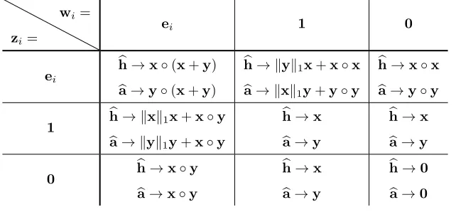
. We summarize in Table1what this implies in practice for the limiting behaviours of hb and ba in (4.3a) and (4.3b) according to the vari-ous possible choices of wi and zi. The limits are reported ignoring global positive multiplicative constants. These do not affect the rankings induced by the centrality vectors, which are the objects of interest in network science. The symbol◦ denotes the entrywise product.
From Table 1 it follows that selecting zi = ei and wi = 0, i.e., a subgraph centrality type of measure, orzi =0and wi=1, i.e., a total node communicability, would return the same ranking in the limit. Indeed,hb will rank the nodes the same asxandbathe same asy. The same is true for all other choices of the vectorszi,wi, apart from whenwi=ei and the trivial choicezi=wi=0.
4 5 6
1 2 3
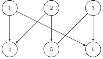
Fig. 1.Example of the network with adjacency matrixAin (6.1) withn= 6.
represented by the adjacency matrix
(6.1) A=
0 B
0 0
∈Rn×n, where B=I+C=
1 1
1 1
1 . .. . .. . ..
1 1
∈Rn2×
n
2,
withneven.
The nodes are ordered in such a way thati→ n
2+ifor alli= 1, . . . ,
n
2,i→
n
2+i−1
for alli= 2, . . . ,n
2 and 1→n. Figure1illustrates the case wheren= 6.
The nodes in this family of networks belong to two distinct groups: they are either sources or targets of edges. Following the notation of Section3.1, we will denote the two groups asS1 ={1,2, . . . , n/2}and S2={n/2 + 1, n/2 + 2, . . . , n}. The network
has been designed so that NBTAWs are forced to explore the network. For example, a NBTAW of lengthnmust involve every node. For largen, eliminating backtracking should help to highlight pairs of nodes that are in the same bipartite group but far apart periodically (such as nodes 1 anddn/4e). By contrast, a backtracking version should give relatively high pairwise weights to nodes in the same bipartite group that are periodically close (such as nodes 1 and 2), since there are many more backtracking walks between them. So, overall, non-backtracking should give a more consistent weighting between all nodes in a bipartite group, especially when the downweighting parameter is large. For the same reason, the NBTAW approach should be less sensitive to perturbations in the structure.
The resolvent-based measures G(A) +G(AT) and
b
G(A) +Gb(AT) are defined in terms of two positive downweighting parameters,αandt. In order for these measures to be well defined, we needα <1/ρ(A) andt <1/ρ(Y), whereY is defined in (4.10). We next show thatρ(A) = 2 andρ(Y) = 1.
The matrixAis unitarily similar to the block-diagonal matrix diag(Σ,−Σ) where Σ is the diagonal matrix containing the singular values of A. It thus follows that ρ(A) =σ1(A). Moreover, because of the structure ofA,σ1(A) =σ1(B) is the leading
singular value of the circulant matrixB. We have
σ1(B) =
q
λ1(BBT) =
q
λ1(2I+C+CT) =
q
2 +λ1(C+CT),
where we assume, here and in the following, that the eigenvalues and singular values are ordered in non-increasing modulus. The eigenvalues of the circulant matrixC+CT areλj = 2 cos(n/2πj2) forj = 1,2, . . . , n/2. Hence, ρ(C+CT) =λ1(C+CT) = 2 and
[image:14.612.171.339.96.193.2]Let us now consider the matrixY, which is permutation-similar to
Y0:=
−I B I I
BT −I
I I I
I
.
Therefore, it follows thatρ(Y) =ρ(Y0) = max{1, ρ(Y[10,1])}, whereY[10,1] denotes the leading 2n×2nblock ofY0. This latter is permutation-similar to
A+AT −I
I 0
,
which is the companion linearization [16] of the matrix polynomial rev(P(t)) associ-ated with the graph represented by A+AT, where P(t) = (1−t2)I−t(A+AT). This graph is simple and connected and all its nodes have degree exactly 2, so that the average degree of the nodes is 2. From [17, Lemma 6.2] it follows that rev(P(t)), and thusY[10,1], hasν distinct finite eigenvaluesλj= exp(−2πνˆιj) forj= 0, . . . , ν−1, whereν is the length of the unique cycle in the graph represented byA+AT. Here, ν=nand thusρ(Y) = 1.
The restrictionsα <1/2 andt <1 may also be understood intuitively by recalling that G(A) is built from the resolvent function. For convergence of the power series, the factorαortmust control any increase in the alternating walk count from length k to k+ 1. If we allow backtracking, then any alternating walk of length k spawns two alternating walks of length k+ 1. Henceα <1/2 is necessary and sufficient to suppress this growth. Eliminating backtracking, only one of these two alternating walks of lengthk+ 1 remains, so the constraint becomest <1.
Test 1. In this first test, we compare the performance ofF(A) +F(AT) (resp.,
G(A) +G(AT)) and
b
F(A) +Fb(AT) (resp.,Gb(A) +Gb(AT)) in highlighting the setsS1
andS2 in a network withn= 60 nodes.
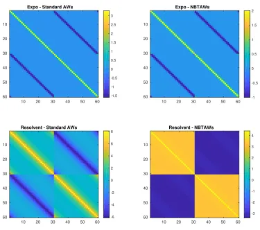
In Figure2we display heatmaps. As discussed in Section3.1, large positive values in the diagonal blocks reveal intra-cluster relationships (S1 → S1 and S2 → S2),
and large negative entries in the off-diagonal blocks reveal inter-cluster relationships (S1→S2 andS2→S1).
In the upper plots we see that both exponential-based measures, F(A) +F(AT) andFb(A) +Fb(AT), show rapid decay away from the diagonal—because the measure emphasizes short walks, pairs of nodes in the same bipartite group that are period-ically far apart are not highlighted. The color bar indicates that this effect is more pronounced for the standard walks.
For the lower plots in Figure2, we see that the resolvent-based measuresF(A) + F(AT) and
b
F(A) +Fb(AT) withα= 0.99/2 andt= 0.99 do a better job of revealing the structure, and in particular the non-backtracking version is able to highlight all types of interaction.
Expo - Standard AWs
10 20 30 40 50 60 10 20 30 40 50 60 -1.5 -1 -0.5 0 0.5 1 1.5 2 2.5 3
Expo - NBTAWs
10 20 30 40 50 60 10 20 30 40 50 60 -1 -0.5 0 0.5 1 1.5 2
Resolvent - Standard AWs
10 20 30 40 50 60 10 20 30 40 50 60 -6 -4 -2 0 2 4 6
8 Resolvent - NBTAWs
10 20 30 40 50 60 10 20 30 40 50 60 -3 -2 -1 0 1 2 3 4
Fig. 2. Upper: heatmaps ofF(A) +F(AT)and b
F(A) +Fb(AT). Lower: heatmaps ofG(A) + G(AT)(α= 0.99/2) and
b
G(A) +Gb(AT)(t= 0.99).
= 0.25/2
20 40 60 10 20 30 40 50 60 0 0.5 1 1.5 2
t = 0.25
20 40 60 10 20 30 40 50 60 0 0.5 1 1.5 2 = 0.5/2
20 40 60 10 20 30 40 50 60 0 0.5 1 1.5 2
t = 0.5
20 40 60 10 20 30 40 50 60 -0.5 0 0.5 1 1.5 2 = 0.8/2
20 40 60 10 20 30 40 50 60 -0.5 0 0.5 1 1.5 2 2.5
t = 0.8
20 40 60 10 20 30 40 50 60 -0.5 0 0.5 1 1.5 2 = 0.99/2
20 40 60 10 20 30 40 50 60 -5 0 5
t = 0.99
20 40 60 10 20 30 40 50 60 -2 0 2 4
[image:16.612.68.443.93.425.2] [image:16.612.72.443.473.657.2]Test 2. We now quantify the resilience of these methods to noise, in the form of spurious edges that impair the bipartite structure. More precisely, we successively added an extra directed edge to the network up to a limit of 60 edges. Each new edge was chosen uniformly at random, with the condition that repeated edges and loops are not allowed. After each edge had been added, we computed the symmetric matrices G(A) +G(AT) and Gb(A) +Gb(AT) for the new adjacency matrix A. To break the network into two groups, we used a standard spectral clustering approach [19,34]— we computed the eigenvector v[1] associated with the dominant eigenvalue λ1 and
assigned node iand node j to the same group ifv[1]i and vj[1] shared the same sign. This splits the nodes into two groups. In order to judge the algorithms, we regarded the group with the mostS1 nodes as our approximation toS1={1,2, . . . , n/2 = 30}
and the other group as our approximation to S2 = {n/2 + 1, n/2 + 2, . . . , n = 60}.
Note that the algorithm was not forced to place 30 nodes in each group; we were not hard-wiring the group size into the tests.
We assessed performance with the F1 score, which is the harmonic average of precision and recall:
F1 = 2precision ×recall precision + recall.
The F1 score ranges between 0 and 1, with 1 representing perfect precision and recall. Recall that precision is the ratio of the number of relevant items to the number of those selected by the method, so
precision = True Positive
True Positive + False Positive,
whilst recall (or sensitivity) is the ratio of the number of relevant items selected to the overall number of relevant items, and thus
recall = True Positive
True Positive + False Negative.
In more detail, we display the F1 score relative to the identification of the nodes in the set S1. In this case, precision is the ratio between the number of positive (or
negative) entries found in the top 30 entries of the eigenvector considered, i.e., the correctly identify nodes, and the total number of its entries with that sign. The recall, on the other hand, is the ratio of the number of correctly identified nodes to the size of S1. (Clearly, good performance with respect toS1 corresponds to good performance
with respectS2.)
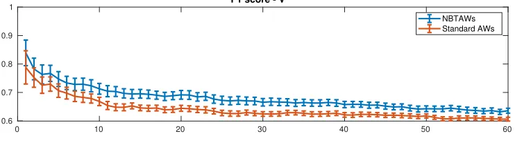
We ran this test 250 times and averaged the results. In Figures 4–6 we display the evolution of the average F1 score with the number of updates performed, with standard errors appended. We are not displaying here results on precision and recall considered individually, as we observed that their averages over 250 runs in this test case behave rather similarly. Therefore, their harmonic mean, i.e., the F1 score, well represents the behaviour of both.
0 10 20 30 40 50 60 0.6
0.7 0.8 0.9 1
F1 score - V
NBTAWs Standard AWs
Fig. 4. Evolution of the F1 score of the partition induced by the eigenvectors associated with
the leading eigenvalues ofG(A) +G(AT)and b
G(A) +Gb(AT). Hereαandtare chosen to be0.25 of their upper limits.
0 10 20 30 40 50 60
0.6 0.7 0.8 0.9 1
F1 score - V
NBTAWs Standard AWs
Fig. 5. Evolution of the F1 score of the partition induced by the eigenvectors associated with
the leading eigenvalues ofG(A) +G(AT)and b
G(A) +Gb(AT). Hereαandtare chosen to be0.5of their upper limits.
that these choices take greater account of longer walks, which have more opportunities to backtrack. In particular, with very small parameter values we emphasize walks of length one, which cannot backtrack.
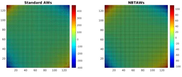
7. Experiment with Worm Brain Data. We now test the performance of the measure Fb(A) +Fb(AT) on a real network. We use a local subnetwork of 131 nodes from the nematode (roundworm)Caenorhabditis elegans. Here, nodes represent neurons and edges reflect physical connections. This network was analyzed in [13] using F(A) +F(AT). A directed bipartite substructure was discovered and shown to be consistent with know attributes of the neurons. The authors identified two sets S1 and S2 of 16 nodes each that constitute an approximate directed bipartite
subgraph in the network: the density of the submatrix S1 →S2 being at least five
times larger that ofSi →Si, fori= 1,2 and S2→S1. A heatmap of the reordered
F(A) +F(AT) is displayed on the left in Figure 7 and the hot zones in the upper left and lower right corners correspond to the indices associated with the nodes inS1
andS2, respectively. On the right in Figure7we display a heatmap of the reordered
b
F(A) +Fb(AT). The two hot regions represent two setsSb1 andSb2 containing 24 and
16 nodes, respectively. The density of the submatrixSb1 →Sb2 is 4, 16, and 32 times
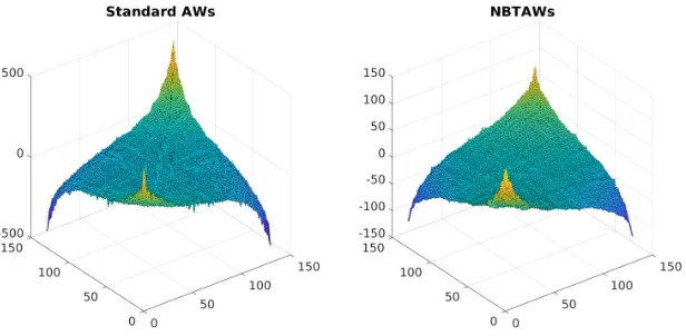
the densities of the submatricesSb1 →Sb1, Sb2→Sb2, andSb2→Sb1. Figure8 displays
[image:18.612.78.440.77.197.2] [image:18.612.71.442.254.359.2]0 10 20 30 40 50 60 0.6
0.7 0.8 0.9 1
F1 score - V
NBTAWs Standard AWs
Fig. 6. Evolution of the F1 score of the partition induced by the eigenvectors associated with
the leading eigenvalues ofG(A) +G(AT)and Gb(A) +Gb(AT). Hereαandtare chosen to be0.99 of their upper limits.
Fig. 7. Heatmap of the reordered version ofF(A) +F(AT)(left) and b
F(A) +Fb(AT)(right), reordered using the entries of the eigenvector associated with its largest eigenvalue.
In summary, the new non-backtracking version of the algorithm has discovered larger and denser directed bipartite substructure than the original method.
8. Summary. Our aim in this work was to combine two concepts that have proved useful in the development of walk-based algorithms for networks: non-backtracking
allows the network to be explored more thoroughly andalternatingreveals bipartite or hub/authority structures. We developed the required combinatoric theory for count-ing non-backtrackcount-ing alternatcount-ing walks and showed that convenient expressions can be derived for the associated power series. This enabled efficient algorithms to be devised—the backtracking constraint essentially imposes no extra cost. We also de-rived the parameter-free limit of the resolvent-based hub/authority measure, giving an analogue of the classical spectral measures.
REFERENCES
[1] N. Alon, I. Benjamini, E. Lubetzky, and S. Sodin. Non-backtracking random walks mix faster. Communications in Contemporary Mathematics, 09:585–603, 2007.
[image:19.612.72.442.84.205.2] [image:19.612.109.410.285.413.2]Fig. 8.Surface plot of the reordered version ofF(A) +F(AT)(left) and of b
F(A) +Fb(AT)(right)
a graph.Transactions of the American Mathematical Society, 326:4287–4318, 2015. [3] F. Arrigo and M. Benzi. Edge modification criteria for enhancing the communicability of
digraphs.SIAM Journal on Matrix Analysis and Applications, 37(1):443–468, 2016. [4] F. Arrigo, M. Benzi, and C. Fenu. Computation of generalized matrix functions.SIAM Journal
on Matrix Analysis and Applications, 37(3):836–860, 2016.
[5] F. Arrigo, P. Grindrod, D. J. Higham, and V. Noferini. On the exponential generating function for non-backtracking walks.Linear Algebra and its Applications, 556:381–399, 2018. [6] F. Arrigo, P. Grindrod, D. J. Higham, and V. Noferini. Non-backtracking walk centrality for
directed networks. Journal of Complex Networks, 6(1):54–78, 2018.
[7] M. Benzi, E. Estrada, and C. Klymko. Ranking hubs and authorities using matrix functions. Linear Algebra and its Applications, 438(5):2447–2474, 2013.
[8] M. Benzi and C. Klymko. Total communicability as a centrality measure. Journal of Complex Networks, 1(2):124–149, 2013.
[9] M. Benzi and C. Klymko. On the limiting behavior of parameter-dependent network centrality measures.SIAM Journal on Matrix Analysis and Applications, 36:686–706, 2015. [10] C. Bordenave, M. Lelarge, and L. Massouli´e. Non-backtracking spectrum of random graphs:
community detection and non-regular ramanujan graphs. Foundations of Computer Sci-ence (FOCS), 2015 IEEE 56th Annual Symposium on, 1347–1357, 2015.
[11] R. Bowen and O. E. Lanford. Zeta functions of restrictions of the shift transformation. In S.-S. Chern and S. Smale, editors,Global Analysis: Proceedings of the Symposium in Pure Mathematics of the Americal Mathematical Society, University of California, Berkely, 1968, pages 43–49. American Mathematical Society, 1970.
[12] R. A. Brualdi, F. Harary, and Z. Miller. Bigraphs versus digraphs via matrices. Journal of Graph Theory, 4(1):51–73, 1980.
[13] J. J. Crofts, E. Estrada, D. J. Higham, and A. Taylor. Mapping directed networks. Electronic Transactions on Numererical Analysis, 37:337–350, 2010.
[14] F. De Ter´an, F. M. Dopico, and P. Van Dooren. Matrix polynomials with completely prescribed eigenstructure.SIAM Jorunal on Matrix Analysis and Applications, 36:302–328, 2015. [15] E. Estrada and D. J. Higham. Network properties revealed through matrix functions. SIAM
Review, 52:696–671, 2010.
[16] I. Gohberg, P. Lancaster, and L. Rodman.Matrix Polynomials. SIAM, Philadelphia, PA, 2009. [17] P. Grindrod, D. J. Higham, and V. Noferini. The deformed graph Laplacian and its applications to network centrality analysis.SIAM Journal on Matrix Analysis and Applications, 39(1), 2018.
[18] J. B. Hawkins and A. Ben-Israel. On generalized matrix functions. Linear and Multilinear Algebra, 1(2):163–171, 1973.
[19] D. J. Higham, G. Kalna, and J. K. Vass. Spectral analysis of two-signed microarray expression data.Mathematical Medicine and Biology, 24(2):131–148, 2007.
[image:20.612.106.414.105.256.2][21] M. D. Horton. Ihara zeta functions on digraphs.Linear Algebra and its Applications, 425:130– 142, 2007.
[22] M. D. Horton, H. M. Stark, and A. A. Terras. What are zeta functions of graphs and what are they good for? In G. Berkolaiko, R. Carlson, S. A. Fulling, and P. Kuchment, editors, Quantum graphs and their applications, volume 415 ofContemp. Math., pages 173–190. 2006.
[23] T. Kawamoto. Localized eigenvectors of the non-backtracking matrix. Journal of Statistical Mechanics: Theory and Experiment, 2016:023404, 2016.
[24] J. M. Kleinberg. Authoritative sources in a hyperlinked environment. Journal of the ACM (JACM), 46(5):604–632, 1999.
[25] F. Krzakala, C. Moore, E. Mossel, J. Neeman, A. Sly, L. Zdeborov´a, and P. Zhang. Spectral redemption: clustering sparse networks.Proceedings of the National Academy of Sciences, 110:20935–20940, 2013.
[26] T. Martin, X. Zhang, and M. E. J. Newman. Localization and centrality in networks. Physical Review E, 90:052808, 2014.
[27] Y. Nakatsukasa, V. Noferini, and A. Townsend. Vector spaces of linearizations of matrix polynomials: a bivariate polynomial approach. SIAM Journal on Matrix Analysis and Applications, 38(1):1–29, 2016.
[28] R. Pastor-Satorras and C. Castellano. Distinct types of eigenvector localization in networks. Scientific Reports, 6:18847, 2016.
[29] Y. Saad. Analysis of some Krylov subspace approximations to the matrix exponential operator. SIAM Journal on Numerical Analysis, 29(1):209–228, 1992.
[30] A. Saade, F. Krzakala, and L. Zdeborov´a. Spectral clustering of graphs with the Bethe Hessian. In Z. Ghahramani, M. Welling, C. Cortes, N. D. Lawrence, and K. Q. Weinberger, editors, Advances in Neural Information Processing Systems 27, pages 406–414. 2014.
[31] H. Stark and A. Terras. Zeta functions of finite graphs and coverings.Advances in Mathematics, 121(1):124–165, 1996.
[32] A. Tarfulea and R. Perlis. An Ihara formula for partially directed graphs. Linear Algebra and its Applications, 431:73–85, 2009.
[33] H. Taubig. Matrix Inequalities for Iterative Systems. CRC Press, 2017.
[34] A. Taylor, J. K. Vass, and D. J. Higham. Discovering bipartite substructure in directed net-works. LMS Journal of Computation and Mathematics, 14:72–86, 2011.
[35] A. Terras. Harmonic Analysis on Symmetric Spaces — Euclidean Space, the Sphere, and the Poincar´e Upper Half-Plane. Springer, New York, 2nd edition, 2013.