entropy
ISSN 1099-4300 www.mdpi.com/journal/entropyArticle
Detecting Chronotaxic Systems from Single-Variable Time
Series with Separable Amplitude and Phase
Gemma Lancaster1, Philip T. Clemson1, Yevhen F. Suprunenko1,2, Tomislav Stankovski1and Aneta Stefanovska1,*
1 Department of Physics, Lancaster University, LA1 4YB, Lancaster, UK
2 Institute of Integrative Biology, University of Liverpool, L69 7ZB, Liverpool, UK
*Author to whom correspondence should be addressed; E-Mail: [email protected].
Academic Editor: Carlo Cafaro
Received: 22 April 2015 / Accepted: 10 June 2015 / Published: 23 June 2015
Abstract: The recent introduction of chronotaxic systems provides the means to describe nonautonomous systems with stable yet time-varying frequencies which are resistant to continuous external perturbations. This approach facilitates realistic characterization of the oscillations observed in living systems, including the observation of transitions in dynamics which were not considered previously. The novelty of this approach necessitated the development of a new set of methods for the inference of the dynamics and interactions present in chronotaxic systems. These methods, based on Bayesian inference and detrended fluctuation analysis, can identify chronotaxicity in phase dynamics extracted from a single time series. Here, they are applied to numerical examples and real experimental electroencephalogram (EEG) data. We also review the current methods, including their assumptions and limitations, elaborate on their implementation, and discuss future perspectives.
Keywords: chronotaxic systems; inverse approach; nonautonomous dynamical systems; Bayesian inference; detrended fluctuation analysis
1. Introduction
observed in nature suggests that previous approaches to the characterization of temporal fluctuations in these observations may be insufficient. At first glance, biological fluctuations may appear random, leading to their description by stochastic models [2]. The complexity observed in biological systems has also led to attempts to treat them with chaos theory [3], however this does not allow for the apparent stability of these systems, irrespective of their initial conditions. Such characteristics of biological oscillators suggests underlying determinism or control of both their amplitudes and frequencies, even with continuous perturbations. This phenomenon of biological systems resisting a natural tendency to disorder was discussed in terms of free energy minimization [4] and separation of internal and external states, but this approach is still based on random dynamics. A closely related, yet more natural, approach is to consider them as nonautonomous systems, which are explicitly time-dependent. Approaches based on reformulation of nonautonomous systems as higher dimensional autonomous systems introduce unnecessary complexity, whilst failing to accurately describe dynamics arising from nature due to the fact that these are open systems, subject to continuous variable external perturbations. Many living systems may be considered as nonautonomous oscillatory systems, with such time-varying dynamics observed in individual mitochondria [5], the cardio-respiratory system [6,7], the brain [8], and blood flow [9].
Although stability of the amplitude dynamics of an oscillator can be achieved with autonomous self-sustained limit cycle oscillators, the frequency of this oscillation could be easily changed by weak external perturbations [10]. To account for a case where this frequency of oscillation is also robust to perturbations, yet time-dependent, a completely new approach is required. Thus, nonautonomous systems with stable, yet time-varying frequencies were recently addressed, and formulated as chronotaxic systems [10–12]. Chronotaxic systems possess a time-dependent point attractor provided by an external drive system. This allows the frequency of oscillations to be prescribed externally through this driver and response system, giving rise to determinism, even when faced with strong perturbations.
2. Chronotaxic Systems
The crucial concept in the theory of chronotaxic systems is the ability to resist continuous external perturbations. In autonomous systems, such an ability is provided by a stationary steady state, allowing the system to always return to the vicinity of this steady state when continuously externally perturbed. However, only in nonautonomous (thermodynamically open) systems can the position of this steady state change in time,i.e., be outside of equilibrium. In such a case, not only the stationary state of a system, but also its time-dependent dynamics will be able to resist continuous external perturbations. These oscillatory nonautonomous dynamical systems with time-dependent steady states were introduced by Suprunenko et al. [10] and named chronotaxic systems, emphasizing that their dynamics is ordered in time (chronos— time,taxis— order).
Mathematically, nonautonomous dynamical systems and, consequently, chronotaxic systems, are defined by the following system of equations:
˙
p=f(p); x˙ =g(x,p), (1)
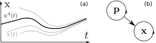
where p ∈ Rn, x ∈ Rm, f : Rn → Rn, g : Rm ×Rn → Rm, in which n andm can be any positive integers. Importantly, the solution x(t, t0,x0) of Equation (1) depends on the actual time t as well as on the initial conditions (t0,x0), whereas the solution p(t −t0,p0) depends only on initial condition p0 and on the time of evolutiont−t0. The subsystemx is nonautonomous in the sense that it can be described by an equation which depends on time explicitly, e.g.,x˙ =g(x,p(t)). A chronotaxic system is described byxwhich is assumed to be observable, andpwhich may be inaccessible for observation, as often occurs when studying real systems. Rather than assuming or approximating the dynamics ofp, we focus on the dynamics ofxand use only the following simple assumption: systemp is assumed to be such that it creates a time-dependent steady state in the dynamics ofx, which is schematically shown in Figure1a.
(a) (b)
Figure 1. (a)Moving point attractor,(b)simplest case of a chronotaxic system.
Therefore, the whole external environment with respect toxis divided into two parts. The first part is given by p which is only that part which makes the system xchronotaxic (defined below), i.e., an unperturbed chronotaxic system. The second part contains the rest of the environment, and is therefore considered as external perturbations.
Firstly, we provide a mathematical formulation of unperturbed chronotaxic systems. The defining component of an unperturbed chronotaxic system is a time-dependent steady state, also called a point attractor, and denotedxA(t).
[image:3.595.174.424.526.595.2]x0 at timet0 the solution of the system asymptotically approaches the time-dependent steady statexA, a condition of forward attraction forxAis the following,
lim
t→+∞|x(t, t0,x0)−x
A(t)|= 0. (2)
This condition can only be satisfied when the chronotaxic system is not perturbed. However, taking into account the time-dependence of xA(t), this condition is not satisfactory in terms of defining the time-dependent point attractor. Any solution ex(t, t0,x0) which satisfies Equation (2) with given xA(t) can also be considered as a time-dependent point attractor. Moreover, when dealing with living systems, it is crucially important to describe stability at the current time t and not in the infinite future. This problem is resolved by employing a condition of pullback attraction, which should also be satisfied by
xA(t)in a chronotaxic system,
lim
t0→−∞
|x(t, t0,x0)−xA(t)|= 0. (3)
One can see, that this condition defines a time-dependent point attractor at current timet.
Considering the condition in Equation (3) at all timest > −∞, it follows that the time-dependent point attractor should also satisfy the invariance condition,i.e., the condition thatxAis a solution of the system Equation (1),
x(t, t0,xA(t0)) =xA(t). (4)
Equations (2) and (3) determine asymptotic convergence in the infinite future or starting from the infinite past. Asymptotic convergence allows the dynamics of x(t, t0,x0) to deviate from xA during a certain finite time interval. Thus, during this time-interval the ability to resist continuous external perturbations will be absent. Therefore, in order to characterize the ability of living systems to sustain their time-dependent dynamics at finite time intervals, a chronotaxic system should satisfy the condition of contraction, or equivalently the attraction at all times. This means that in the phase spaceRm,x∈Rm, there should be a contraction regionC(t)such that for any two trajectoriesx1,x2 of a system inside the contraction regionxi(t, t0,x0i)∈C(t),i= 1,2, the distance between them can only decrease,
d
dt|x1(t, t0,x1,0)−x2(t, t0,x2,0)|<0. (5) However, in general the contraction region C(t) can be finite, and different trajectories can eventually leave this region. Therefore, in a chronotaxic system the contraction region should contain a finite area A0, A0 ⊂ C, such that solutions of the system starting in A0 never leave it, ∀t0 < t, ∀x0 ∈ A0(t0), x(t, t0,x0)∈A0(t).
In such a case, fulfillment of these conditions guarantees that the time-dependent point attractorxAis located inside the areaA0 inside the contraction regionC.
Alternatively, the trajectory xA(t) can be viewed as a linearly attracting uniformly hyperbolic trajectory [13], so that the distance between a neighboring trajectory and xA(t) can only decrease in an unperturbed chronotaxic system. For more details and for relations between chronotaxic and other dynamical systems see Reference [12]. A simple example of an unperturbed chronotaxic system is given by unidirectionally coupled phase oscillators with unwrapped phase ϕx ∈ (−∞,∞)driven by a phase ϕp ∈(−∞,∞):
˙
whereϕ˙p(t) = ω(t).
The point attractor will exist if the condition of chronotaxicity [11] is fulfilled,|ε(t)|>|ω0(t)−ω(t)|. As an example, for a particular choiceε(t) =ω(t)>0andω0(t) = 0, the equation can be integrated, and the limit t0 → −∞can be calculated, leading to the explicit expression for a time-dependent point attractor of an unperturbed chronotaxic system,ϕAx(t) = ϕp(t)−π/2 + 2πk, andk is any integer.
It should be noted that the dynamics ofp can be complex, stochastic, or chaotic, provided that the above conditions are met. Nevertheless, the dynamics of xwill be determined by the dynamics of p, and therefore it will be deterministic, at least in unperturbed chronotaxic systems. When considering perturbed chronotaxic systems, for simplicity it is sufficient to consider perturbations only to the x
component, as any perturbations to p can be included in its dynamics assuming that x does not influence p. In perturbed chronotaxic systems, which model real life systems, the general external perturbations will create complex dynamics of x with a stochastic component. Such dynamics may look very complex: perturbations can push trajectories away from the contraction region, therefore they can temporarily deviate before they converge. Despite this, due to the existence of the contraction region, the system will resist continuous external perturbations. The time-dependent dynamics of a perturbed chronotaxic system will be very close to the dynamics of the unperturbed chronotaxic system provided the perturbations are weak enough. In the case of very strong continuous perturbations, such perturbations may override the driving systemp, and become effectively a new driver, causing the initial point attractor of the chronotaxic system to disappear. However, it may be restored once the perturbations again become sufficiently weak.
Thus, when perturbations do not destroy the chronotaxic properties of a system, the stable deterministic component of its dynamics can be identified, as will be shown below. This reduces the complexity of the system, allowing us to filter out the stochastic component and focus on deterministic dynamics and interactions between system x and its driver p, [10,14]. For such complex systems as living systems, it has the potential to extract properties of the system which were previously neglected.
3. Inverse Approach for Chronotaxic Systems
3.1. Inverse Approaches to Nonautonomous Dynamical Systems
systems appear very complex in phase space. To incorporate time-dependence into these systems, extra dimensions in phase space are required, introducing unnecessary complexity to the problem.
In the case that there is only one oscillation in the time series, the Hilbert transform can be applied to obtain the complex analytic signal, from which the instantaneous phase can be determined directly. If the time series contains more than one component of interest, for example different oscillatory modes, it can be decomposed into its constituent parts using a method such as empirical mode decomposition (EMD), in which peak/trough detection is used to create upper and lower envelopes. From these, a trend is defined and subtracted from the signal to produce a series of intrinsic mode functions, each one representing an oscillatory component of the time series [15]. However, there are some limitations when applying EMD to nonstationary data.
Many signal analysis methods assume stationarity of the frequency distribution of the data, but in nonautonomous systems this assumption is not valid. Single variable time series, particularly those from living systems, must be treated as arising from nonautonomous dynamical systems, due to time-dependent influences of variables other than the one under study. Approaches based on windowing have been applied in order to attempt to treat time variability in data, but these potentially lose crucial information. For example, in phase space reconstruction the window may not be of a sufficient size to capture the whole of the attractor, or its variations in time. Application of the Fourier transform to nonstationary data will result in a blurred or misleading power spectra, severely limiting its usefulness. The windowing approach has been applied here with some success, in the form of the Short Time Fourier transform (STFT), but the use of windowing leads to limitations; the better the time resolution, the worse the frequency resolution (known as the Gabor limit [16]). In addition, the fixed time–frequency relationship at all scales in a windowed Fourier transform severely limits its usefulness for the analysis of low frequency oscillations. This problem can be addressed by using the continuous wavelet transform (CWT), which provides a logarithmic frequency scale (see Section3.3). The CWT is based on wavelets rather than the sines and cosines used in Fourier based methods. The simultaneous observation of the time and frequency domains is extremely useful in the visualization of dynamical systems and their time evolution. As a result, development of wavelet-based methods specifically for the treatment of time-dependent dynamics is now a very active field of research [15], including wavelet phase coherence [17], the synchrosqueezed transform [18,19] and wavelet bispectrum.
and quantified using wavelet bispectrum [22]. The ability of these methods to directly take into account the time-varying characteristics of data makes them ideal for application to nonautonomous systems.
3.2. Detecting Chronotaxicity
Here we present two distinct inverse approach methods which may be utilised in the detection of chronotaxicity: phase fluctuation analysis (PFA) and dynamical Bayesian inference. It should be noted that the current methods are only applicable to phase dynamics in the context of the detection of chronotaxicity, i.e., we focus on the ability of the time-varying frequency to resist continuous external perturbations. The two methods rely on a different inferring basis. Phase fluctuation analysis provides a measure of statistical effects observed in a signal, whilst the dynamical Bayesian inference method infers a model of differential equations and gives a measure of dynamical mechanisms, i.e., the evaluation of chronotaxicity relies on the inferred parameters of the model. PFA is said to infer a functional connectivity, while the dynamical Bayesian inference method infers effective connectivity [23]. The optimal method to use depends on the characteristics of the data, as detailed below.
It is possible to detect whether a system is chronotaxic or not by observing the distribution of the fluctuations in the system relative to its unperturbed trajectory. This comes from the fact that if the original distribution of the perturbations is known, then the stability of the system relative to the unperturbed trajectory (which by definition follows the time-dependent point attractor in a chronotaxic system) can be determined from how these perturbations grow or decay over time. For example, take the non-chronotaxic phase oscillator [24]
˙
ϕx =ω0(t) +η(t), (7)
where ω0(t) is the time-dependent natural frequency and the observed phaseϕx is perturbed by noise fluctuationsη(t). Integrating we find,
ϕx=
Z
ω0(t)dt+
Z
η(t)dt. (8)
Assuming that ω0(t) > 0 and η(t) is an uncorrelated Gaussian process, this means that the dynamics of ϕx will consist of a monotonically increasing phase perturbed by a random walk noise (Brownian motion). However, the situation is different for a chronotaxic phase oscillator, e.g.,
˙
ϕp =ω0(t), (9)
˙
ϕx =εω0(t) sin(ϕp−ϕx) +η(t),
3.3. Extracting the Perturbed and Unperturbed Phases
The first problem of generating a method based on the above principle is how to extract both the perturbed and unperturbed phases of the system from an observed time series. This usually requires the separation of the amplitude and phase for an oscillation in the time series, which is possible using time–frequency domain analysis [15]. The analytic signal generated by the Hilbert transform can also be used, but this requires corrections for nonlinear oscillations and cannot be used when more than one oscillation is present in the time series [14,25,26]. Additionally, the use of the Hilbert transform requires the use of protophase-to-phase conversion [26].
A time–frequency representation with an optimal frequency resolution of the time seriesf(t)of length Lis provided by the continuous wavelet transform [27],
WT(s, t) = Z L
0
Ψ(s, u−t)f(u)du, (10)
whereΨ(s, t)is the mother wavelet, which is scaled according to the parametersto change its frequency distribution and time-shifted according tot. The Morlet wavelet is a commonly used mother wavelet and is defined as [28],
Ψ(s, t) = √41
π
e2πifs0t −e−
2πf02
2
e−t
2
2s2, (11)
where the corresponding frequency is given by 1/sand f0 is a parameter known as central frequency which defines the time/frequency resolution [27].
Oscillations can be traced in WT(s, t) using either a ridge-extraction method [29,30] or the synchrosqueezed wavelet transform (SWT) [18]. These extraction methods can be used to estimate the instantaneous frequencies of the oscillatory components in a time series, allowing identification of harmonics, which can be used to determine the intra-cycle dynamics. The phase ϕx of the observed system is thenarg(WT(s, t)), wheresandtdenote the positions of the oscillation in thes−tplane.
With the estimated perturbed phaseϕ∗x extracted, further work is needed to obtain the unperturbed phaseϕA∗
x . In particular, it is difficult to separate the dynamics corresponding toϕAx from the effect of the noise perturbations η(t). This task is simplified by assuming that the dynamics ofϕAx are confined to time scales larger than a single cycle and that the noise is either weak or comparable in magnitude to these dynamics.
With these assumptions, an estimate ofϕA
x can be found by filtering out high frequency components ofϕ∗x. However, such a filter should not smooth over the dynamics ofϕAx. An optimal way of removing these high frequency noise fluctuations without affecting the unperturbed dynamics is to instead smooth over the frequency extracted from the wavelet transform [15]. This provides the estimated angular velocity ϕ˙A
x, which can in turn be integrated over time to give the estimated phase of the driver ϕA
∗
x . For further methodological details on phase extraction see Section4.2.
3.4. Dynamical Bayesian Inference
One approach to the detection of chronotaxicity is the application of dynamical Bayesian inference to the extracted perturbed (ϕ∗x) and unperturbed (ϕA∗
In dynamical systems Bayesian inference can simultaneously detect time-varying synchronization, directionality of coupling and time-evolving coupling functions [20,21]. The characteristics of these coupling functions between ϕ∗x and ϕA∗
x may reveal the dynamic mechanisms of the system in terms of chronotaxicity. Bayesian inference is able to track time-dependent system parameters, meaning that it is particularly useful for the detection of chronotaxicity in systems which move in and out of a chronotaxic state.
Following extraction of phases from the continuous wavelet transform, as described in Section 3.3, we assume their dynamics is described by [14,20,21]
˙
ϕi =ωi+fi(ϕi) +gj(ϕi, ϕj) +ξ(t), (12)
whereωiis the natural frequency of the oscillation,fi(ϕi)are the self-dynamics of the phase,gi(ϕi, ϕj)
are the cross couplings, andξ(t)is a two-dimensional white Gaussian noisehξi(t)ξj(τ)i=δ(t−τ)Eij. Based on the periodic nature of the system, the basis functions are modeled using the Fourier bases
fi(ϕi) =
∞
X
k=−∞ ˜
ai,2ksin(kϕi) + ˜ai,2k+1cos(kϕi), (13)
and
gi(ϕi, ϕj) = ∞
X
s=−∞ ∞
X
r=−∞
˜bi,r,se2πirϕie2πisϕj, (14)
wherek, r, s 6= 0. In practice, it is reasonable to assume that the dynamics will be well described by a finite number of Fourier terms, denotedAi,k(ϕi, ϕj). The corresponding parameters from˜ai and˜bi then form the parameter vectorc(ki). The inference of these parameters utilises Bayes’ theorem,
pX(M|X) =
`(X |M)pprior(M)
R
`(X |M)pprior(M)dM
, (15)
wherepX(M|X)is the posterior probability distribution and`(X |M)is the likelihood function for the
values of the model parametersMgiven the dataX, andpprior(M)is a prior distribution. The negative log-likelihood function is
S = N
2 ln|E|+
h
2
N−1
X
n=0
c(kl)∂Al,k(ϕ.,n) ∂ϕl
+ [ ˙ϕi,n−c (i)
k Ai,k(ϕ.∗,n)](E
−1
)i,j[ ˙ϕj,n−c (j)
k Aj,k(ϕ.∗,n)]
,
(16)
with implicit summation over repeated indices k, l, i, j. The log-likelihood is a function of the Fourier coefficients of the phases [20].
Assuming a multivariate normal distribution as the prior for parameters c(ki) with means ¯c and covariancesΣ = Ξ−1, the stationary point of S can be calculated recursively from
Ei,j = h
N[ ˙ϕi,n−c (i)
k Ai,k(ϕ.
∗
,n)][ ˙ϕj,n−c (j)
k Aj,k(ϕ.
∗
,n)], (17)
c(ki) = (Ξ−1)i,lkwr(wl),
r(wl) = (Ξprior) (i,l) kw c
(l)
w +hAi,k(ϕ.∗,n)(E
−1)
ijϕ˙j,n− h
2
∂Al,k(ϕ.,n) ∂ϕl ,
Ξi,jkw = Ξi,jpriorkw+hAi,k(ϕ.∗,n)(E
−1)
These are calculated within a moving time window, with the current prior depending on information from the posterior of the previous window. The inferred parameters of the basis functions can be used to determine whether synchronization results. The presence of synchronization provides evidence that the system is chronotaxic, however it remains unclear from which coupling function the stability arises without calculating the direction of coupling [31],
D= 12−21
12+21
, (18)
where
12 =
q c2
2+c24+..., (19)
21 =
q
c21+c23+...,
are the Euclidean norms of the parameters. The odd parameters correspond to the coupling terms inferred forϕ1in the direction 2→1, and the even parameters correspond to the coupling terms inferred forϕ2in the direction 1→2. See [32] for further details and an in depth tutorial on dynamical Bayesian inference and its implementation.
In summary, Bayesian inference is applied toϕ∗x andϕAx∗, following their extraction from the time series (see Section 3.3). The time evolution of the coupling parameters for each phase is inferred and these are used to determine the synchronization state of the system, and the direction of coupling between the phases. In a chronotaxic system we require the driver and response systems to be almost or fully synchronized, and also that the direction of coupling is only from the driverϕAx toϕx.
The basis of this method is the calculation of the synchronization and direction of coupling of the system in order to determine chronotaxicity. However, the more synchronized the driver is with the response system, the less information flow between the two. With less information from which to infer parameters, most directionality methods, including Bayesian inference, become less reliable, and whilst synchronization may still be accurately detected, the direction of coupling will become less accurate the closer the system gets to synchronization. With frequent external perturbations, intermittent transitions, and moderate dynamical noise, there is greater information flow, and thus the inference is more precise, but this cannot be assumed in chronotaxic systems. In real systems, the synchronization state is not known beforehand, thus a more robust method is required, which can identify chronotaxicity even in systems close to synchronization.
3.5. Phase Fluctuation Analysis
Phase fluctuation analysis is effective even when ϕx and ϕp are almost synchronized. Given the estimates ofϕxandϕAx, the next step is to analyse∆ϕx=ϕ∗x−ϕA
∗
x to find the distribution of fluctuations in the system relative to the unperturbed trajectory.
time scales equal to t/acan be made similar to those at the larger time scale tby multiplying with the factoraα.
0 2 4 −1
0 1
Chronotaxic
0 2 4 −1
0 1
Non−chronotaxic
0 2 4 −1
0 1
Chronotaxiclwithlphaselslips
250 500 750 −10
0 10
250 500 750 −5
0 5
Timel(s) 250 500 750
−1 0 1 1 2 4 8 2 4 4 8 2 4 4 8 2 4 2 6 2 6 10 20
4 8 12 10
30
4 8 12 10
20
2 6 10 4
8
2 6 10 2 6 0.2 1 2 6 10
(a)
(b)
(c)
(d)
(e)
(f)
(g)
(h)
=l1 =l10 =l25 =l50 =l100
[image:11.595.52.545.128.425.2]=l0.65 =l1.47 =l1.25
Figure 2. (a)–(c) 5 s time series of sin(ϕx) (red line) in 3 cases: chronotaxic, non-chronotaxic, and chronotaxic with phase slips, from Equation (21). The grey line showsϕp(chronotaxic), andωxt(non-chronotaxic). (d)–(f)∆ϕx for the whole time series, detrended with a moving average of 200 s. In all casesωx,p= 2π, h = 0.001, L = 1000 s and σ = 0.3. ε= 5 and 0 in the chronotaxic and non-chronotaxic cases, respectively. detrended fluctuation analysis (DFA) exponents, α, are shown. The DFA exponent of (f)incorrectly suggests the system is non-chronotaxic. To distinguish between a non-chronotaxic system and a chronotaxic system with phase slips, the delayed distributions were calculated (see Section3.5) in the non-chronotaxic(g)and chronotaxic(h)case.
In order to calculateα, the time series∆ϕx is integrated in time and divided into sections of length n. For each section the local trend is removed by subtracting a fitted polynomial—usually a first order linear fit [6,33]. The root mean squarefluctuationfor the scale equal tonis then given by
F(n) =
v u u t 1 N N X i=1
Yn(ti)2, (20)
(expected in non-chronotaxic systems) returns a value of 1.5. Note that this assumes that the noise does not cause phase slips inϕx. This would cause perturbations over large time scales (i.e., greater than one cycle) to not decay even if the system was chronotaxic. In these cases another approach should be used instead [14].
If there are large perturbations which cause the system to move far enough forward or behind the current cycle to be attracted instead by an adjacent cycle, known as a phase slip, this will result in an increased DFA exponent. This can result from large jumps in the extracted phase fluctuations. To distinguish between the case of a chronotaxic system with phase slips, and a non-chronotaxic system, we consider the fact that in the latter, perturbations may cause∆ϕxto change by 2π, but these are part of a continuous probability distribution, in contrast to the chronotaxic case. Phase slips can be detected by calculating the distribution of the difference between the phase fluctuations∆ϕx(t)and these fluctuations delayed by a time scale τ. d∆ϕτ
x(t) = ∆ϕx(t+τ)−∆ϕx(t) therefore gives information about the perturbations of the system over that time scale. When phase slips are present, the distribution of|d∆ϕτ
x| changes with respect toτ [14]. An example of this difference is shown in Figure2g,h, and can also be seen in real biological systems, as previously demonstrated in the heart rate variability [14].
4. Application of Inverse Approach Methods
4.1. Numerical Simulations
The basis of the PFA method is the quantification of the fundamental difference between phase fluctuation distributions in oscillatory systems, depending on their chronotaxicity. Here, we illustrate this characteristic using the simplest realisation of a chronotaxic system, two unidirectionally coupled oscillators (see Figure1b):
˙
ϕp =ωp
˙
ϕx =ωx−εsin(ϕx−ϕp) +η(t), (21)
where ϕp and ϕx are the instantaneous phases of the driving and the driven oscillators, respectively, ωp >0andωx >0are the natural frequencies of the oscillators,ε >0is the strength of the coupling and ηis white Gaussian noise with standard deviationσ =√2E wherehη(t)i= 0,hη(t)η(τ)i=δ(t−τ)E. Note that when ε = 0 the system is reduced to ϕ˙x = ωx +η(t) and becomes non-chronotaxic; when η = 0andε >|ωx−ωp|the system becomes chronotaxic withϕAx(t) =ϕp(t)−arcsin((ωp−ωx)/ε). The system was integrated using the Heun scheme [15], with an integration step of 0.001 and noise strength σ = 0.3. ∆ϕx, shown in Figure2, was obtained by subtracting the unperturbed phase (ϕA
x(t) and ωxt in the chronotaxic and non-chronotaxic cases, respectively) from the perturbed phaseϕx, as obtained numerically. DFA was then performed on ∆ϕx, with exponents shown in Figure 2. The values of the exponents demonstrate the differences in the noise distributions between chronotaxic and non-chronotaxic systems. In the chronotaxic case, the noise is closer to white, whereas in the non-chronotaxic case it is closer to a random walk. It is this difference which is exploited in the PFA method.
multiple modes a signal containing two distinct oscillations was simulated, with dynamics described by Equation (21), with time varying angular frequencies,
˙
ωvar(t) = Acos(2πfmt) +η(t)
ωx,p(t) = 2πfx,p+ωvar, (22)
wherefpandfxare the average frequencies of oscillation in Hz of the chronotaxic and non-chronotaxic case, respectively, andfm is the frequency of variation. Frequencies of oscillation were chosen to vary around 1 and 0.25 Hz in the non-chronotaxic and chronotaxic cases, respectively, withfm= 0.003. Both systems were perturbed with white Gaussian noise with strength σ = 0.5. The logarithmic frequency scale of the wavelet transform is very useful for identifying and separating the presence of oscillatory modes, which may otherwise appear as merged in other time–frequency representations, such as the windowed Fourier transform. Figure 3 shows the results of PFA on the signal. It correctly identifies mode A (around 0.25 Hz) as chronotaxic, and mode B (around 1 Hz) as non-chronotaxic.
(a)
(b) (c)
(d) (e)
[image:13.595.65.541.330.570.2](f) (g)
Figure 3.Identifying chronotaxicity in signals with more than one oscillatory mode.(a)The first 250 s of a time series of a simulated signal containing two distinct oscillations, with coupling strengthsε= 2 for mode A (chronotaxic) andε= 0 for mode B (non-chronotaxic). (b)The continuous wavelet transform of the signal in(a). (c)The instantaneous frequency (light grey) of both components is extracted from the wavelet transform, with central frequency f0 = 0.5, and smoothed (red), using a polynomial fit. The smoothed frequency is then integrated in time to obtain an estimate of the unperturbed phase,ϕA∗
x , which is then subtracted from the perturbed phase ϕ∗x as extracted directly from the wavelet transform. (d)and(e)show ∆ϕx = ϕ∗x−ϕA
∗
x for each mode. (f)and(g)show the results of DFA on
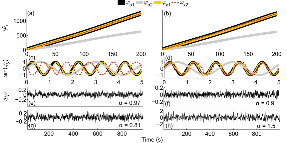
In single variable time series obtained from real dynamical systems, it is highly unlikely that the observed dynamics will result from a simple, unidirectional constant coupling as described above. Rather, the system may be influenced by continuous perturbations, couplings to other oscillators, and temporal fluctuations in chronotaxicity. Here, we demonstrate the applicability of the described inverse approach methods to these more complex cases. We model a system of two bidirectionally coupled oscillators:
˙
ϕp1 =ωp1 (23)
˙
ϕp2 =ωp2
˙
ϕx1 =ωx1 +ε1sin(ϕx1−ϕx2)−ε4sin(ϕx1−ϕp1) +η(t)
˙
ϕx2 =ωx2 +ε2sin(ϕx2−ϕx1)−ε3sin(ϕx2−ϕp2) +η(t),
with driversϕp1andϕp2, andωp1(t) = 2π−0.5 sin(2π0.005(t))andωp2(t) =π−0.5 cos(2π0.005(t)). First, we consider the case of strong influence of the driverϕp1on the system, resulting in chronotaxicity of both oscillators. Phase fluctuation analysis was applied to the system, and successfully identified both ϕx1andϕx2as chronotaxic (see Figure4a).
0 50 100 150 200
0 500 1000
x
0 1 2 3 4 5
−10 1
−0.20 0.2
∆
200 400 600 800 −0.20
0.2
0 50 100 150 200
−0.2 0 0.2
200 400 600 800 −2
0 2
Time (s)
0 1 2 3 4 5
−10 1
sin(
x
)
p1 p2 x1 x2
(a) (b)
(d) (c)
(e) (f)
(g) (h)
α= 0.97 α= 0.9
[image:14.595.65.546.359.598.2]α= 0.81 α= 1.5
Figure 4. Identifying chronotaxicity using phase fluctuation analysis in a system of bidirectionally coupled oscillators. The system presented in Equation (23) was simulated in two different states of chronotaxicity. (a)Phase trajectories for the system whenε1= 0.1, ε2 = 20,ε3 = 0.1 and ε4 = 10. (b)Phase trajectories of the system with ε1 = 0.5, ε2 = 0.1, ε3 = 0.1 andε4 = 15. (c) Five seconds of the time series of both drivers and oscillators for parameters shown in(a). (d) A 5 s time series for parameters shown in(b). (e)and(g)phase fluctuations from PFA onsin(ϕx1)andsin(ϕx2), respectively. (f)and(h)phase fluctuations extracted with PFA onsin(ϕx1)andsin(ϕx2), respectively.
arising from the same system can be distinguished in terms of their chronotaxic dynamics. Again, PFA correctly distinguishes between the two oscillators. This could be of great importance when investigating composite parts of a larger dynamical system, and seeking to identify causal relationships between observed oscillations. For example, recent advances in cellular imaging are providing the means to observe the dynamics of individual cellular processes in different cellular compartments [34]. Applying inverse approach methods for the detection of chronotaxicity to these dynamics could provide valuable information on the current state of the cell.
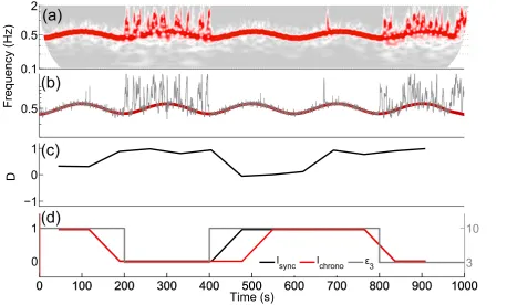
Figure 5. Identifying intermittent chronotaxicity using dynamical Bayesian inference. Bayesian inference was performed on ϕ∗x2 and ϕA∗
x2 extracted from sin(ϕx2) (see Equation (23)) withε3varying as shown in(d). (a)the CWT ofsin(ϕx2). (b)Instantaneous frequencies extracted from the wavelet transform. ϕA∗
x2 was extracted with f0 = 2 and smoothed using a polynomial fit (red line), whilst ϕ∗x2 was extracted from the wavelet transform withf0= 0.5 (grey line). Bayesian inference was applied, using a time window of 90 s. The inferred direction of coupling can be seen in (c). Positive values show coupling from the driver to the oscillator only.(d)Isyncwas calculated and shows excellent agreement
with changes in ε3. Ichrono was also calculated, and was slightly less accurate due to the
direction of coupling becoming negative very briefly, because of reduced information flow between systems to accurately infer parameters during synchronization.
vary in time in Equation (23), whilstε1 = ε2 = 0.1 andε4 = 0, resulting in intermittent chronotaxicity of the oscillator ϕx2. ϕAx2∗ and ϕ
∗
x2 were extracted from the synchrosqueezed wavelet transform of
sin(ϕx2). Results of the application of dynamical Bayesian inference are shown in Figure 5. This method is able to track the intermittent changes in chronotaxicity, through changes in synchronization and direction of coupling, demonstrating its usefulness for the detection of chronotaxicity in systems where the interactions between oscillators are time-varying.
4.2. Practical Considerations
Both presented methods, phase fluctuation analysis and dynamical Bayesian inference, rely on precise phase extraction of the estimated attractorϕA∗
x and the perturbed dynamicsϕ
∗
x. Therefore, the parameters in the respective methods must be carefully selected depending on the characteristics of the given data.
The continuous wavelet transform provides an optimal compromise between time and frequency resolution. In the majority of examples used in this paper,f0 = 1 has been used. However, the wavelet central frequency, f0, can be altered to suit specific needs. For example, in a case where there are many phase slips, it may be necessary to extract the estimate of the attractor, ϕA∗
x , with a higherf0 to obtain a better frequency resolution and smoother dynamics, whilst the perturbed phaseϕ∗xis extracted using a lowerf0, leading to an increased time resolution for the purpose of locating each phase slip. The parameterf0may also be increased to provide greater distinction between oscillatory modes, but this will be at the expense of time resolution. It should be noted that modes must be separable in time–frequency representations in order for these inverse approach methods to be applicable.
provides ϕAx∗for use in phase fluctuation analysis. ϕ∗xcan then be extracted from the wavelet transform as before, with the parameterf0chosen to give sufficient time resolution to follow the noise fluctuations which are removed by NMD. An example of the use of NMD in PFA is provided in Figure 6, and explained further in Section4.3.
0 200 400 600 800 1000 1200
−100
0 100
Frequ
encyz(Hz)
1 10
0 200 400 600 800 1000 1200
5 10 15
0 200 400 600 800 1000 1200
0 5
xz104
300 320 340 360 380 400
−4
−20
2 4 6
2 4 0
2000
=z1
2 4 =z10
2 4 =z50
2 4 =z100 1
10
Timez(s)
Timez(s)
(a)
(b)
(c)
(d)
(e)
(f)
(g)
=z1.57
(b)
(c)
[image:17.595.54.551.167.450.2]20 20
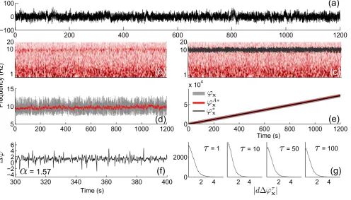
Figure 6. An example of the application of phase fluctuation analysis to an electroencephalogram (EEG) signal obtained from the forehead of an anaesthetised patient, shown in (a). (b) The continuous wavelet transform of the electroencephalogram (EEG) signal in(a).(c)Using NMD, a significant oscillatory mode in the alpha frequency band was identified and extracted (dark grey line). (d) The instantaneous frequency extracted using NMD (grey line), and smoothed using a moving average of 4 s (red line). (e)The extracted phases of the mode from NMD (grey), smoothed NMD (red), and from the CWT (black) with f0 = 1.5. (f) ∆ϕx was calculated as ϕ∗x − ϕA
∗
x . The DFA exponent was calculated and was 1.57, suggesting that the system is not chronotaxic. Checking for phase slips in(g) shows no change in distribution.
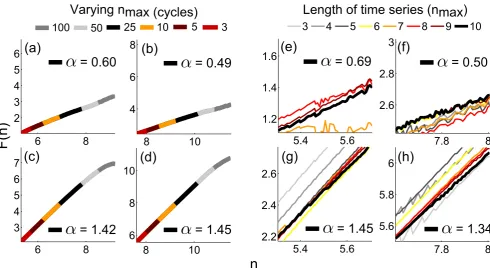
In order to address this question, two unidirectionally coupled phase oscillators (Equation (21)) were simulated for 1000 cycles with frequencies 1 and 0.1 Hz, with h = 0.01 and σ = 0.07. With coupling ε= 2, the system is chronotaxic. The important parameters to consider in DFA are nmin and nmax, the
lower and upper values for the range of the first order polynomial fits performed in order to calculate
∆ϕx. The lower value, nmin, is set to be 2 cycles of the slowest oscillation, to ensure observation of the
dynamics over a longer range than one cycle. The smallest nmax required to still obtain a reliable DFA
exponent was observed to be nmax = 3 cycles of oscillation (see Figure7), provided that the time series
[image:18.595.53.544.229.497.2]is sufficiently long. The second test seeks to identify the required length of the whole time series when
Figure 7. In order to test the reliability of the DFA exponent when reducing nmax, the
maximum number of cycles of oscillation used in its calculation was varied.(a)Chronotaxic oscillation of 1 Hz. (b)Chronotaxic oscillation of 0.1 Hz. (c)Non-chronotaxic oscillation of 1 Hz. (d)Non-chronotaxic oscillation of 0.1 Hz. The same noise signals were then tested with nmax = 3 for different lengths of the time series from 10 to 3 times nmax. Based on
these results, the time series should be at least 8 times nmax, thus, there should be at least
24 oscillations in the time series. However, to ensure universal applicability, the length of the time series should be at least 10 times nmax, the generally accepted value in DFA [38],
resulting in the requirement of 30 cycles.
using these values of nminand nmaxin DFA. The DFA exponent was calculated from varying lengths of the
same noise signals, from 3 to 10 times nmax, to identify the point where the result is no longer reliable. It
was found that the time series should be at least 8 times nmaxin order to obtain a reliable result, therefore
at least 24 cycles of the slowest oscillation are required to test for chronotaxicity. However, if possible, the time series should be at least 10 times nmax[38], to reduce noise by providing more data windows.
Whilst we expect the value of the DFA exponent α to be around 0.5 in a chronotaxic system, and 1.5 in a non-chronotaxic system, it is unlikely to be so definitive in reality. In fact, the value of α will depend on a number of factors. The type of noise in a real system is not necessarily white, however the point of phase fluctuation analysis is to identify changes in its distribution. αwill also vary depending on how strong the chronotaxicity is in the system, i.e., how strongly driven the observed oscillator is. In our models, this can be represented by varying the coupling strength ε; weaker coupling will result in a higher DFA exponent as the noise is partially integrated. The ratio of the natural frequency of the chronotaxic oscillator to the frequency of the external driver, or detuning, may also affect the value ofα.
4.3. Application to Experimental Data
Chronotaxicity will manifest in nature as a result of a driving system which is strong enough that the oscillatory response system maintains stability in its frequency and amplitude, even when subject to continuous external perturbations. Chronotaxicity was previously demonstrated in the heart rate variability (HRV) [14], when influenced by paced breathing. It has been shown that the main direction of coupling between the cardiac and respiratory oscillators is the influence of the respiration on the heart rate, known as respiratory sinus arrhythmia (RSA), and this was clearly demonstrated. Here, we provide an example of the application of phase fluctuation analysis to real experimental data in the form of an electroencephalogram (EEG) recording from an anaesthetised human subject.
determines the degree of excitability of the neurons, and influences precise discharge times of the cells in the network, therefore affecting relative timing of action potential in different brain regions [42].
Before any conclusions may be drawn about the phase dynamics of a system, the phase must be accurately extracted from the time series. The problem of the extraction of phase from EEG data has been approached from many directions, some more physically meaningful than others. Early approaches to the investigation of phase interactions between brain waves used spectral coherence, but this does not separate phase and amplitude components, thus amplitude effects may influence coherence values when only phase locking information is required [43]. A widely used phase extraction approach is the use of the Hilbert transform to obtain the analytic signal [44], usually preceded by band-pass filtering in the frequency interval of interest, highlighting the necessity of the separation of the oscillation of interest from background brain activity—either other oscillations or noise. Lachaux, et al. recognised the necessity of the separation of amplitude and phase when seeking to detect synchrony between brain waves, introducing phase-locking statistics (PLS) [43] to measure the phase covariance between two signals, verified by surrogate testing. This method also allows for non-stationarity in the signal. However, based on very narrow band-pass filtering, this method does not allow for time-variability in the frequency of oscillation, but did highlight the usefulness of complex wavelets in the extraction of phase dynamics. The Hilbert transform and wavelet convolution methods were compared in the analysis of neural synchrony, and found not to differ substantially [45], but both of these methods relied on narrow band-pass filtering beforehand. However, the use of band-pass filtering to extract an oscillatory EEG component with a time-varying frequency has limited usefulness. An instantaneous frequency defined from the analytic signal obtained from band-passing in a particular frequency range in a real signal containing multiple spectral components and noise may be ambiguous and meaningless [41]. To address this problem, ridge extraction methods [29] applied to the complex wavelet transform were used to track the instantaneous frequency of a single oscillatory mode [41], providing a much higher precision of phase extraction, and importantly allowing the phase dynamics of nonautonomous systems to be accurately traced in time. Another rarely considered issue when tracing instantaneous frequencies in time is the presence of high harmonics in the signal. Narrow restriction of the frequency range will remove these harmonics, and thus remove valuable intra-cycle phase information. This issue has been addressed directly by the introduction of nonlinear mode decomposition [35]. The inverse approach methods applied here take into account all these issues in order to accurately extract the instantaneous phase of brain oscillations.
the continuous wavelet transform with a time resolution which will allow the noise fluctuations to be included in the extracted mode. Here, it is very important to check that the extracted phase corresponds to that extracted using NMD (see Figure6e). Once the viability of the extracted fluctuations is confirmed,
∆ϕxcan be calculated asϕ∗x−ϕA
∗
x . The DFA exponent of∆ϕxwas then calculated, and was 1.57. The distribution |d∆ϕτx|was calculated to check for phase slips in the extracted phase fluctuations, but the distribution did not change over any time scaleτ.
The analysis suggests that the alpha oscillation as extracted is not chronotaxic. However, the current inverse approach methods are based on a single point attractor and a single response system. As discussed by Sheppard,et al. [46], the spectral peaks observed in the EEG, including those observed in the alpha band, result from frequency synchronization between thousands of neurons. In this sense, the observed phase is, in fact, only a statistical measure highlighting the preferred phase of the underlying ensemble of neurons. A method to quantify this was provided by the mean-field variability index, κ, which changes depending on the interactions in the observed network of oscillators [46]. For a non-interacting network, with purely random phasors, κ will converge to 0.215, whereas in a state of complete phase synchronization,κwill tend to zero. Based on the current assumptions of the inverse approach methods, if the detection of chronotaxicity relied only on phase dynamics, we would expect the value of κ to tend to zero in a chronotaxic system. However, when applied to real EEG data, κ was actually greater than 0.215 in most cases, suggesting amplitude synchrony (possibly intermittent), intermittent phase coherence, or both. Therefore, it is apparent that in the case of brain dynamics, to truly characterise chronotaxicity, it must be reconsidered within a network of many oscillators, as known to be present in the brain. Here, the driving system may be a subnetwork of synchronized oscillators or the mean-field or mean-phase of ensembles of neurons, influencing other areas of the brain in complex ways, with both temporal and spatial dynamics to take into account.
5. Discussion
The recent formulation of chronotaxic systems provides a completely novel approach to the characterisation of time-varying dynamics in real data. Crucially, they provide a framework in which systems may be time-varying, both in terms of their amplitude and phase dynamics, continuously perturbed, and yet still exhibit determinism. Whilst the apparent complexity of some real time-varying oscillatory systems previously led to their consideration as stochastic or chaotic, chronotaxicity facilitates a much more natural approach to the description of their dynamics. The introduction of this approach required the development of new inverse approach methods for the detection of chronotaxicity in time series arising from dynamical systems. Here, we reviewed the currently available methods for the identification of chronotaxicity from a single time series, and also expanded on various issues regarding their implementation, in order to facilitate the application of the methods to any data set containing at least one oscillatory component. This ability to characterise oscillations in terms of their chronotaxicity, i.e., to determine whether the observed dynamics arise as a result of influence from an external driver, provides the potential to unlock new information about dynamical systems and their interactions with their environment.
As they currently stand, the inverse approach methods for the detection of chronotaxicity are only applicable to systems in which the amplitude and phase dynamics are separable, as they are applied directly to the extracted phases of the system and all amplitude information is discarded. This assumption is valid if considering that the amplitude dynamics of a chronotaxic system corresponds to the convergence of the system to the limit cycle, influenced only by a negative Lyapunov exponent and external perturbations. In contrast, the phase dynamics corresponds to convergence to the time-dependent point attractor, which is also characterized by a negative Lyapunov exponent and external perturbations, but also the motion of the point attractor itself [14]. As it is this point attractor in phase dynamics that we are interested in—separation of amplitude and phase follows naturally. Using this approach, an example of chronotaxic dynamics was succesfully demonstrated in a real system, in the case of heart rate variability [14]. However, in generalized chronotaxic systems [12], the amplitude and phase are not required to be separable, providing even greater applicability to real systems, allowing amplitude–amplitude and amplitude–phase interactions in addition to the phase–phase dynamics considered in [10,11]. Therefore, the incorporation of the ability to identify these new possibilities for chronotaxicity is crucial in the further development of these inverse approach methods. This will then provide the means to detect chronotaxicity in systems where amplitude and phase are not separable, as previously discussed in the case of brain dynamics (see Section4.3). The current definition of chronotaxicity is based on a time-varying point attractor, exerting influence over a system such that it can remain stable despite continuous external perturbations. Numerical results presented here assume that this point attractor results from a single oscillatory drive system acting on a maximum of two coupled oscillators. However, as highlighted in the brain dynamics example, in reality we must consider that this point attractor could result from multiple interacting influences, for example a network of oscillators, perhaps acting as one synchronized drive system.
their phase and amplitude dynamics with utmost accuracy. Methods reliant on averaging will not provide the required precision. Both amplitude and phase information can be extracted from the continuous wavelet transform, a fact which may be utilised in the further development of inverse approach methods for the detection of chronotaxicity. Extending these methods to simultaneously take into account both phase and amplitude dynamics whilst incorporating the effects of their couplings, may lead to a method based on an optimal combination of time–frequency representations and effective connectivity methods such as dynamical Bayesian inference. This will then provide even wider applicability to real oscillatory systems such as those observed in brain dynamics.
Acknowledgments
This work was supported by the Engineering and Physical Sciences Research Council (UK) (Grant No. EP/100999X1) and in part by the Slovenian Research Agency (Program No. P20232).
Author Contributions
Aneta Stefanovska conceived the research. Gemma Lancaster performed the analysis, prepared the figures, and with Philip Clemson and Yevhen Suprunenko wrote the manuscript. Tomislav Stankovski was involved in the implementation of dynamical Bayesian inference. All authors have read, commented on, and approved the final manuscript.
Conflicts of Interest
The authors declare no conflict of interest.
References
1. Kloeden, P.E., Pöetzsche, C., Eds. Nonautonomous Dynamical Systems in the Life Sciences; Springer: Cham, Switzerland, 2013; pp. 3–39.
2. Friedrich, R.; Peinke, J.; Sahimi, M.; Tabar, M.R.R. Approaching Complexity by Stochastic Methods: From Biological Systems to Turbulence.Phys. Rep. 2011,506, 87–162.
3. Wessel, N.; Riedl, M.; Kurths, J. Is the Normal Heart Rate “Chaotic” due to Respiration? Chaos 2009,19, 028508.
4. Friston, K. A Free Energy Principle for Biological Systems.Entropy2012,14, 2100–2121.
5. Kurz, F.T.; Aon, M.A.; O’Rourke, B.; Armoundas, A.A. Wavelet Analysis Reveals Heterogeneous Time-Dependent Oscillations of Individual Mitochondria. Am. J. Physiol. Heart Circ. Physiol. 2010,299, H1736–H1740.
6. Shiogai, Y.; Stefanovska, A.; McClintock, P.V.E. Nonlinear Dynamics of Cardiovascular Ageing. Phys. Rep. 2010,488, 51–110.
8. Stam, C.J. Nonlinear Dynamical Analysis of EEG and MEG: Review of an Emerging Field. Clin. Neurophysiol. 2005,116, 2266–2301.
9. Stefanovska, A.; Braˇciˇc, M.; Kvernmo, H.D. Wavelet Analysis of Oscillations in the Peripheral Blood Circulation Measured by Laser Doppler Technique.IEEE Trans. Bio. Med. Eng. 1999,46, 1230–1239.
10. Suprunenko, Y.F.; Clemson, P.T.; Stefanovska, A. Chronotaxic Systems: A New Class of Self-sustained Non-autonomous Oscillators. Phys. Rev. Lett.2013,111, 024101.
11. Suprunenko, Y.F.; Clemson, P.T.; Stefanovska, A. Chronotaxic Systems with Separable Amplitude and Phase Dynamics.Phys. Rev. E2014,89, 012922.
12. Suprunenko, Y.F.; Stefanovska, A. Generalized Chronotaxic Systems: Time-Dependent Oscillatory Dynamics Stable under Continuous Perturbation. Phys. Rev. E2014,90, 032921.
13. Bishnani, Z.; Mackay, R.S. Safety Criteria for Aperiodically Forced Systems.Dyn. Syst.2003,18, 107–129.
14. Clemson, P.T.; Suprunenko, Y.F.; Stankovski, T.; Stefanovska, A. Inverse Approach to Chronotaxic Systems for Single-Variable Time Series.Phys. Rev. E2014,89, 032904.
15. Clemson, P.T.; Stefanovska, A. Discerning Non-autonomous Dynamics. Phys. Rep. 2014, 542, 297–368.
16. Gabor, D. Theory of Communication.J. Inst. Electr. Eng. 1946,93, 429–457.
17. Sheppard, L.W.; Vuksanovi´c, V.; McClintock, P.V.E.; Stefanovska, A. Oscillatory Dynamics of Vasoconstriction and Vasodilation Identified by Time-Localized Phase Coherence. Phys. Med. Biol. 2011,56, 3583–3601.
18. Daubechies, I.; Lu, J.; Wu, H.T. Synchrosqueezed Wavelet Transforms: An Empirical Mode Decomposition-Like Tool.Appl. Comput. Harmon. Anal.2011,30, 243–261.
19. Iatsenko, D.; McClintock, P.V.E.; Stefanovska, A. Linear and Synchrosqueezed Time-Frequency Representations Revisited: Overview, Standards of Use, Resolution, Reconstruction, Concentration and Algorithms.Digit. Signal Process.2015,42,1–26.
20. Stankovski, T.; Duggento, A.; McClintock, P.V.E.; Stefanovska, A. Inference of Time-Evolving Coupled Dynamical Systems in the Presence of Noise. Phys. Rev. Lett.2012,109, 024101. 21. Duggento, A.; Stankovski, T.; McClintock, P.V.E.; Stefanovska, A. Dynamical Bayesian Inference
of Time-Evolving Interactions: From a Pair of Coupled Oscillators to Networks of Oscillators. Phys. Rev. E2012,86, 061126.
22. Jamšek, J.; Paluš, M.; Stefanovska, A. Detecting Couplings between Interacting Oscillators with Time-Varying Basic Frequencies: Instantaneous Wavelet Bispectrum and Information Theoretic Approach. Phys. Rev. E2010,81, 036207.
23. Friston, K. Functional and Effective Connectivity: A Review.Brain Connect. 2011,1, 13–36. 24. Kuramoto, Y.Chemical Oscillations, Waves, and Turbulence; Dover: New York, NY, USA, 2003. 25. Oppenheim, A.V.; Schafer, R.W.; Buck, J.R.Discrete-Time Signal Processing, 2nd ed; Prentice
Hall: Upper Saddle River, NJ, USA, 1999.
26. Kralemann, B.; Cimponeriu, L.; Rosenblum, M.; Pikovsky, A.; Mrowka, R. Phase Dynamics of Coupled Oscillators Reconstructed from Data. Phys. Rev. E2008,77, 066205.
28. Morlet, J. Sampling Theory and Wave Propagation. InIssues in Acoustic Signal-Image Processing and Recognition; Chen, C.H. Ed.; Springer: Berlin/Heidelberg, Germany, 1983; pp. 233–261. 29. Delprat, N.; Escudie, B.; Guillemain, P.; Kronland-Martinet, R.; Tchamitchian, P.; Torrésani, B.
Asymptotic Wavelet and Gabor Analysis: Extraction of Instantaneous Frequencies. IEEE Trans. Inf. Theory1992,38, 644–664.
30. Carmona, R.A.; Hwang, W.L.; Torrésani, B. Characterization of Signals by the Ridges of their Wavelet Transforms.IEEE Trans. Signal Process.1997,45, 2586–2590.
31. Rosenblum, M.G.; Pikovsky, A.S. Detecting Direction of Coupling in Interacting Oscillators.Phys. Rev. E.2001,64, 045202.
32. Stankovski, T; Duggento, A; McClintock, P.V.E.; Stefanovska, A. A Tutorial on Time-Evolving Dynamical Bayesian Inference.Eur. Phys. J. Spec. Top. 2014,223, 2685–2703.
33. Peng, C.K.; Buldyrev, S.V.; Havlin, S.; Simons, M.; Stanley, H.E.; Goldberger, A.L. Mosaic Organisation of DNA Nucleotides.Phys. Rev. E1994,49, 1685–1689.
34. Kioka, H.; Kato, H.; Fujikawa, M.; Tsukamoto, O.; Suzuki, T.; Imamura, H.; Nakano, A.; Higo, S.; Yamazaki, S.; Matsuzaki, T.;et al.Evaluation of Intramitochondrial ATP Levels Identifies GO/G1 Switch Gene 2 as a Positive Regulator of Oxidative Phosphorylation. Proc. Natl. Acad. Sci. USA 2014,111, 273–278.
35. Iatsenko, D.; McClintock, P.V.E.; Stefanovska, A. Nonlinear Mode Decomposition: A Noise-Robust, Adaptive Decomposition Method.Phys. Rev. E2015, in press.
36. Vejmelka, M.; Paluš, M.; Šušmáková, K. Identification of Nonlinear Oscillatory Activity Embedded in Broadband Neural Signals. Int. J. Neural Syst.2010,20, 117–128.
37. Paluš, M.; Novotná, D. Enhanced Monte Carlo Singular System Analysis and Detection of Period 7.8 years Oscillatory Modes in the monthly NAO Index and Temperature Records.Nonlinear Proc. Geoph. 2004,11, 721–729.
38. Hardstone, R.; Poil, S.S.; Schiavone, G.; Jansen, R.; Nikulin, V.V.; Mansvelder, H.D.; Linkenkaer-Hansen, K. Detrended Fluctuation Analysis: A Scale-Free View on Neuronal Oscillations. Front. Physiol. 2012,3, 450.
39. Klimesch, W. EEG Alpha and Theta Oscillations Reflect Cognitive and Memory Performance: A Review and Analysis.Brain Res. Rev. 1999,29, 169–195.
40. Purdon, P.L.; Pierce, E.T.; Mukamel, E.A.; Prerau, M.J.; Walsh, J.L.; Wong, K.F.K.; Salazar-Gomez, A.F.; Harrell, P.G.; Sampson, A.L.; Cimenser, A.; et al. Electroencephalogram Signatures of Loss and Recovery of Consciousness from Propofol. Proc. Natl. Acad. Sci. USA 2013,110, E1142–E1151.
41. Rudrauf, D.; Douiri, A.; Kovach, C.; Lachaux, J.P.; Cosmelli, D.; Chavez, M.; Adam, C.; Renault, B.; Martinerie, J.; Le Van Quyen, M. Frequency Flows and the Time-Frequency Dynamics of Multivariate Phase Synchronization in Brain Signals.Neuroimage2006,31, 209–227.
42. Fell, J.; Axmacher, N. The Role of Phase Synchronization in Memory Processes. Nat. Rev. Neurosci. 2011,12, 105–118.
44. Tass, P.; Rosenblum, M.G.; Weule, J.; Kurths, J.; Pikovsky, A.; Volkmann, J.; Schnitzler, A.; Freund, H.J. Detection of n:m Phase Locking from Noisy Data: Application to Magnetoencephalography. Phys. Rev. Lett.1998,81, 3191–3294.
45. Le Van Quyen, M.; Foucher, J.; Lachaux, J.P.; Rodriguez, E.; Lutz, A.; Martinerie, J.; Varela, F.J. Comparison of Hilbert Transform and Wavelet Methods for the Analysis of Neural Synchrony. J. Neurosci. Methods2001,111, 83–98.
46. Sheppard, L.W.; Hale, A.C.; Petkoski, S; McClintock, P.V.E.; Stefanovska, A. Characterizing an Ensemble of Interacting Oscillators: The Mean-Field Variability Index. Phys. Rev. E 2013, 87, 012905.
47. Palva, S.; Palva, J.M. New Vistas forα-Frequency Band Oscillations. Trends Neurosci. 2007,30, 150–158.
48. Stankovski, T.; Ticcinelli, V.; McClintock P.V.E.; Stefanovska, A. Coupling Functions in Networks of Oscillators.New J. Phys.2015,17, 035002.
49. Sauseng, P.; Klimesch, W. What does Phase Information of Oscillatory Brain Activity Tell us about Cognitive Processes? Neurosci. Biobehav. R.2008,32, 1001–1013.
50. Darvas, F.; Miller, K.J.; Rao, R.P.N.; Ojemann, J.G. Nonlinear Phase-Phase Cross-Frequency Coupling Mediates Communication between Distant Sites in Human Neocortex.J. Neurosci.2009, 29, 426–435.
51. Tort, A.B.L.; Komorowski, R.; Eichenbaum, H.; Kopell, N. Measuring Phase-Amplitude Coupling between Neuronal Oscillations of Different Frequencies.J. Neurophysiol. 2010,104, 1195–1210. 52. Friston, K.J. Another Neural Code?Neuroimage1997,5, 213–220.
53. Hurtado, J.M.; Rubchinsky, L.L.; Sigvardt, K.A. Statistical Method for Detection of Phase-Locking Episodes in Neural Oscillations. J. Neurophysiol.2004,91, 1883–1898.
54. Lisman, J.E.; Jensen, O. The Theta-Gamma Neural Code.Neuron2013,77, 1002–1016.
55. Canolty, R.T.; Knight, R.T. The Functional Role of Cross-Frequency Coupling. Trends Cogn. Sci. 2010,14, 506–515.
56. Mukamel, E.A.; Pirondini, E.; Babadi, B.; Foon Kevin Wong, K.; Pierce, E.T.; Harrell, P.G.; Walsh, J.L.; Salazar-Gomez, A.F.; Cash, S.S.; Eskandar, E.N.; et al. A Transition in Brain State during Propofol-Induced Unconsciousness. J. Neurosci.2014,34, 839–845.
c