promoting access to White Rose research papers
Universities of Leeds, Sheffield and York
http://eprints.whiterose.ac.uk/
This is an author produced version of a paper published in Journal of Electron Spectroscopy and Related Phenomena.
White Rose Research Online URL for this paper:
http://eprints.whiterose.ac.uk/8712/
Published paper
Beamson, G., Mokarian-Tabari, P. and Geoghegan, M. (2009) Composition depth profiling of polystyrene/poly(vinyl ethyl ether) blend thin films by angle resolved XPS. Journal of Electron Spectroscopy and Related Phenomena, 171 (1-3). pp. 57-63.
Accepted Manuscript
Composition depth profiling of polystyrene / poly(vinyl ethyl ether) blend
thin films by angle resolved XPS.
G.Beamson1*, P.Mokarian-Tabari2and M.Geoghegan2.
1. National Centre for Electron Spectroscopy and Surface Analysis (NCESS), STFC
Daresbury Laboratory, Warrington, Cheshire. WA4 4AD, UK.
2. Department of Physics and Astronomy, University of Sheffield, Hounsfield Road,
Sheffield. S3 7RH, UK.
* Corresponding author. Tel.: +44 1925 603 479; fax: +44 1925 603 596. E-mail address:
Keywords.
Polystyrene, poly(vinyl ethyl ether), thin film polymer blend, angle resolved XPS, scanning
force microscopy, composition depth profile.
Abstract.
Angle resolved XPS (ARXPS) and scanning force microscopy (SFM) are used to study
polystyrene / poly(vinyl ethyl ether) 50 / 50 wt% blend thin films spin cast from toluene
solution, as a function of polystyrene molecular weight and film thickness. ARXPS is used to
investigate the composition depth profile (CDP) of the blend thin films and SFM to study their
surface morphology and miscibility. The CDPs are modelled by an empirical hyperbolic
tangent function with three floating parameters. These are determined by non-linear least
squares regression, their uncertainties estimated and the curve fit residuals analysed to
demonstrate that the hyperbolic tangent CDP is a satisfactory fit to the ARXPS data.
Conclusions are drawn regarding the behaviour of the blend thin films as the thickness and
polystyrene molecular weight are varied. Flory-Huggins interaction parameters () for the
Accepted Manuscript
mixtures are calculated based upon the segregation data, and suggest a value of= 0.05 to
be appropriate for this system.
1. Introduction.
The behaviour of polymer blend thin films is often significantly different from that of the same
materials in the bulk and is important in applications such as paints, adhesives, polymer
based electronics and biocompatible coatings. Particular phenomena of interest are the
preferential segregation of blend components to interfaces, phase separation,
wetting/dewetting, film stability, pattern formation and thin film confinement effects [1-3].
Hence for both fundamental and applied reasons the surface and interface regions of polymer
blend thin films have been studied intensively for many years using depth profiling and
microscopy techniques. For example, neutron reflectometry [4] and MeV ion scattering [5]
have been used to provide composition depth profile (CDP) information, and scanning force
microscopy (SFM) has been used to study surface morphology [6-8]. Polymer blend thin films
are often prepared by spin casting from solvent onto a suitable substrate, as this allows
straightforward control of film thickness via solution concentration and rotation speed, and
studied as a function of film thickness [9, 10] and molecular weight (MW) [11-13].
X-ray photoelectron spectroscopy (XPS) can provide elemental composition and chemical
speciation information from the near surface region of a polymer sample [14-18] and when
combined with ion sputtering can provide CDP information, although with reduced knowledge
of chemical speciation due to the destructive nature of the sputtering process. Angle resolved
XPS (ARXPS) can also be used to investigate the CDP of a sample between ~ 1 and ~ 8 nm
Accepted Manuscript
34] and Cumpson [35] has shown how uncertainties in the intensity measurements limit the
information that can be extracted from the data. The measured photoelectron intensity from a
particular core level of a particular species is given by [20]:
K is the product of various instrumental factors, is the photoionization cross-section, F is the
spectrometer transmission, c(z) is the concentration of the species as a function of depth z,
i.e. the CDP, is the photoelectron inelastic mean free path and is the photoelectron
take-off-angle measured relative to the sample surface. A set of angle resolved XPS data consists
of measurements of I() at several values of , typically between 5 and 10, and recovery of
c(z) amounts to taking the inverse Laplace transform of the angle resolved data set. This can
be achieved numerically but the problem is fundamentally “ill-conditioned” and very sensitive
to noise in the data, i.e. to the uncertainties in the intensity measurements. For realistic signal
/ noise ratios of ~ 100 only three parameters relating to the CDP can be reliably extracted
from the data [35]. Thus care needs to be exercised in the interpretation of CDP parameters
determined from ARXPS and estimates made of the uncertainties in those parameters. A
number of methods are available for carrying out the inverse Laplace transform but it is
generally accepted that the best procedure is to use the least squares method to fit a model
of the CDP based on prior knowledge to the experimental ARXPS data [24, 27, 33, 35].
Here we describe a study of polystyrene / poly(vinyl ethyl ether) (PST / PVEE) blend thin films I() = KF c(z). exp(-z / sin). dz (1)
0
Accepted Manuscript
much studied polystyrene / poly(vinyl methyl ether) (PST / PVME) blend system [29-31,36-39] but with a less favourable Flory-Huggins interaction parameter. (The Flory-Huggins
interaction parameter, usually denoted , is a dimensionless and temperature-dependent
measure of the interaction energy between two components relative to their energies in their
own melts. The -parameter, along with the MWs of the chains is all that is needed to define
the miscibility of a polymer blend at a given composition using the regular solution theory of
polymer mixtures [40].) This has been attributed to greater shielding of the interaction
between the ether oxygen atom and the aromatic ring by the ethyl group of PVEE compared
with the methyl group of PVME [41]. The less favourable interaction causes PST / PVEE
blends to change from miscible to phase separated as the PST MW increases. PVEE
preferentially segregates to the blend surface and we describe the use of ARXPS to
investigate the CDPs of the blend thin films and of SFM to study their surface morphology and
hence miscibility. We assume that the CDPs can be modelled by an empirical hyperbolic
tangent function [42] described by three floating parameters. These are determined by
non-linear least squares regression, their uncertainties estimated and the curve fit residuals
analysed to demonstrate that the hyperbolic tangent CDP is a satisfactory fit to the ARXPS
data. Conclusions are drawn regarding the behaviour of the blend thin films as the thickness
and PST MW are varied and Flory-Huggins interaction parameters are calculated for each
film, based upon the CDP.
Systematic uncertainties often dominate random ones in determining the accuracy of an XPS
analysis [35, 43] and we describe steps taken to minimise the effect of x-ray induced sample
damage [44] during our experiments and to investigate the effect of contaminants present in
Accepted Manuscript
ARXPS study of an electrically insulating polymer sample is the need to maintain good charge
compensation, and hence spectral resolution, as is varied.
2. Experimental.
The x-ray photoelectron spectra were recorded using a Scienta ESCA300 spectrometer. This
employs a high power rotating anode and monochromatised Al Kx-ray source (h = 1486.7
eV), high transmission electron optics and a multichannel detector [45, 46]. The geometry of
the x-ray source, sample manipulator and electrostatic lens is such that at low the x-ray
beam strikes the sample at glancing incidence. This gives enhanced sensitivity at low and is
ideal for the study of thin film samples [45]. The scale of the spectrometer was calibrated by
recording Si 2p spectra of a piece of silicon wafer as a function of the angle setting of the
sample manipulator and measuring the angle at which the Si(0)/Si(IV) ratio was a maximum,
which corresponds to = 90o. For C 1s photoelectrons and the instrument settings used in
this work the angular acceptance of the ESCA300 lens is ~ +/- 3o[47]. The energy scale of
the spectrometer was regularly checked using the Fermi edge, 3d5/2 and M4VV lines of a
sputter cleaned sample of silver foil, and the measured binding energies came within 0.1 eV
of the corresponding literature values (0.0, 368.26 and 1128.78 eV respectively) [48]. Spectra
were recorded at 150 eV pass energy and 0.8 mm slit width, giving an overall instrument
resolution of ~ 0.35 eV [49]. The x-ray source power was 2.8 kW and charge compensation
was achieved using a Scienta FG300 low energy electron flood gun. The step interval of the
region spectra was 0.05 eV.
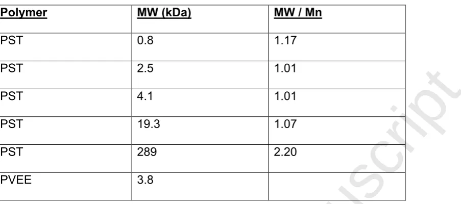
Details of the polymers used for preparation of the blend thin films are shown in Table 1. All
Accepted Manuscript
accurate weighing into clean glass vials. Solutions of pure PST and pure PVEE, ~ 3 wt% in
toluene, were also prepared. One drop of solution was placed on a 10 mm diameter glass
disk (wiped with tissue / isopropanol) fixed with double sided tape to an XPS sample stub and
mounted on a spin coater. After spinning for ~ 30 seconds at 2000 rpm the samples were
transferred immediately to the vacuum system of the XPS spectrometer. For each blend
solution a first spin cast sample was used to record a survey spectrum at = 90o and a
second, fresh sample, was used to record a sequence of C 1s spectra at = 90o, 75o, 60o,
45o, 30o, 20o and 10o. The sample position was changed systematically between the C 1s
spectra, both to minimise the effect of x-ray induced sample damage and for optimum charge
compensation. The acquisition time for each C 1s spectrum was ~ 2.5 minutes and the effect
of x-ray induced damage on the angle resolved spectra is judged to have been small.
Calibration curves of the PST / PVEE blend film thickness as a function of the concentration
of the toluene solution used for spin casting were generated by spin casting onto silicon wafer
substrates at 2000 rpm and measuring the absorbance of the PST 700 cm-1 line using a
Bio-Rad FTS-60A FTIR spectrometer. The relationship between absorbance and film thickness
was determined by placing a scratch across several pure polystyrene thick film samples and
measuring the depth of the scratch using a step profilometer.
SFM images of blend films on silicon wafer substrates were recorded using a Nanoscope IIIa
(Veeco, Santa Barbara, USA) operated in tapping mode with an OMCL silicon probe from
Olympus. The cantilevers had a nominal spring constant of 40 N / m and a resonant
frequency of 300 kHz. Height and phase data were collected simultaneously and the images
Accepted Manuscript
Thick drop cast films of the PST / PVEE blends were prepared for visual observation of phase
separation by placing several drops of ~ 10 wt% solution in toluene onto 10 mm diameter
glass disk substrates and leaving to dry in air for 2 days. These films are estimated to have
been several hundred microns thick.
3. Data Analysis.
The C 1s spectra of pure PST and PVEE are shown in Figure 1 and a set of angle resolved C
1s spectra for a thin film blend sample is shown in Figure 2. The pure PST spectrum is shown
binding energy referenced to C 1s = 284.8 eV and the PVEE spectrum to the lowest binding
energy C 1s component = 285.0 eV. This brings the second component of the PVEE
spectrum to 286.4 eV, in agreement with previous measurements [14], and the spectra shown
in Figure 2 are binding energy referenced to this value.
For each angle resolved data set (consisting of C 1s spectra at 7 values of ) the areas of the
PST and PVEE spectra (A()PST and A()PVEE) present in the blend spectra were determined
by curve fitting using CasaXPS software [50], with spectra of the pure PST and PVEE films as
basis functions. A typical curve fit is shown in Figure 3. The experimental PVEE apparent
volume fractions were calculated from:
()Expt= A()PVEE (2)
Accepted Manuscript
MPVEE and MPST are the repeat unit molecular weights (72 and 104 Da respectively), 4 / 8 is
the ratio of the number of carbon atoms in the PVEE / PST repeat units and PVEE and PST
are the polymer densities (0.968 and 1.047 g/cm3respectively).
For a binary polymer blend in which one component preferentially segregates to the surface
the CDP in the near surface region, expressed in terms of the volume fraction of the surface
segregating component, (z), can be described by an empirical hyperbolic tangent function
[42]:
s and b are the surface and bulk volume fractions, is related to the thickness of the
surface overlayer (essentially providing a parameter to replicate flattening of the CPD near
the surface [51]) and determines the width of the interface region between the surface and
the bulk; see Figure 4. In PST / PVEE blends PVEE segregates to the surface because of its
lower surface free energy and we assume that s for PVEE is one. This is supported by the
ARXPS data but we note that because the minimum XPS sampling depth (i.e. 3sinat =
10ois ~ 2 nm, the assumption may not be strictly true for all the blend thin films.
Hence, with the CDP of equation (3) PVEE apparent volume fractions can be calculated from:
(z) = b+ (s–b). (1 – tanh((z –)/)) (3) (1 – tanh(–/))
()Calc= (z). exp(-z / sin). dz exp(-z / sin). dz (4)
0
t t
Accepted Manuscript
Within an Excel 2003 spreadsheet trial initial values of b, and were used to calculate (z)
from equation (3) and then ()Calc at each of the experimental values by numerical
integration of equation (4). For films thicker than 20 nm the upper limit of the integration, t,
was set equal to 20 nm, whereas for thinner films it was set equal to the film thickness. For all
films dz = t/1000. For C 1s photoelectrons excited by Al Kradiation moving through PST /
PVEE was taken as 3.7 nm [52]. This model neglects elastic scattering effects which have
been shown to be small for PST [20].
The final values of b, and were determined by minimisation of the sum of square
differences: (()Expt – ()Calc)2 (i.e. summed over the 7 experimental values) using the
Solver non-linear optimisation routine [53]. The standard deviations of b, and and the
coefficient of determination, R2, were calculated using the Solvstat macro [54]. This is
equivalent to using the curve fit residuals to calculate the uncertainties in the CDP
parameters, as discussed by Cumpson [35].
The curve fit values of b, and were used to calculate angle resolved profiles from
equations (3) and (4) for comparison with the experimental data points, as shown in Figures
5a), 6a) and 7a). For one data set, out of the total of 18, comparison of the experimental
points and the curve fit line revealed an obvious single outlier point; this was eliminated and
Solver + Solvstat re-run. For four other data sets, where the range of () on going from =
90o to 10o was small, Solver produced low and obviously erroneous values for b, and in
these cases it was fixed at a more appropriate value (see Section 4.2) and Solver + Solvstat
Accepted Manuscript
For each angle resolved data set the residual at each data point was calculated from:and the mean and standard deviation of the residuals calculated for the data set.
To simulate the effect of different levels of noise in the experimental data a hyperbolic tangent
composition depth profile with defined values of b, and was used to calculate () at =
90o, 75o, 60o, 45o, 30o, 20oand 10o, and random noise added to the data points such that the
standard deviation of the noise was equal to a certain fraction of (), e.g. 0.5%. Solver was
then used to re-calculate the values of b, and , and the procedure repeated 10 times in
order to obtain standard deviations for the re-calculated values.
4. Results and discussion.
4.1 SFM.
Thick drop cast samples of PST / PVEE blends are transparent for PST MW = 0.8 and 2.5
kDa and opaque for PST MW >= 4.1 kDa. The SFM data (Figure 8) reveal that for spin cast
blend films ~ 100 nm thick only those with PST MW = 289 kDa have a rough surface
topography (RMS roughness ~ 11.7 nm) indicating that they are phase separated, the
surfaces of the other films being rather smooth (RMS roughness ~ 0.3 - 0.8 nm) indicating
that they are miscible. In addition, spin cast films with PST MW = 289 kDa become smooth
when the thickness is reduced to 30 and 12 nm (RMS roughness ~ 0.5 nm). For an
incompatible polymer blend system (Hmix > 0) the reduction in the entropy of mixing (Smix)
with increasing MW causes Gmix = Hmix - TSmix (where T is the absolute temperature) to
Accepted Manuscript
become positive above a certain MW and phase separation to occur rather than mixing [3].
For the thick drop cast samples this transition is between PST MW = 2.5 and 4.1 kDa,
whereas for the ~ 100 nm spin cast films it is between 19.3 and 289 kDa. Hence confinement
of the PST / PVEE blends in thin film geometry appears to shift the transition from miscible to
immiscible to higher MW. Similar thin film confinement effects have been observed in other
polymer blend systems [6, 55-59]. On the basis of the SFM data we propose that the spin
cast blend thin films with PST MW = 0.8, 2.5 and 4.1 kDa are miscible and that their angle
resolved C1s data can be analysed using a hyperbolic tangent composition depth profile as
described in section 3. The spin cast blend thin films with higher PST MW are either
immiscible (289 kDa) or close to immiscible (19.3 kDa) and analysis of their angle resolved C
1s data is omitted.
4.2 XPS.
In addition to C and O the survey spectra of some of the thicker blend films spin cast onto
glass substrates show a very low level of Si (~0.1 at% for films spin cast from ~ 10 wt%
solutions in toluene, i.e. ~ 250 nm thick) probably due to the surface segregation of silicone
contamination present in the bulk of the films. Interestingly, survey spectra of thick drop cast
samples (many hundreds of microns thick) reveal significant Si contamination, e.g. ~ 5 at% for
the blend with PST Mw = 4.1 kDa. This shows that although silicone contamination is present
in the blends at rather low overall concentration the thick drop cast films contain enough
material to give a high surface concentration of Si. However, for the spin cast films of interest
here the film thicknesses are sufficiently small that the surface concentration of Si is almost
undetectable. The survey spectra of blend films spin cast from dilute solutions in toluene, i.e.
Accepted Manuscript
The experimental and curve fit angle resolved profiles for blends with PST MW = 0.8, 2.5 and
4.1 kDa are shown in Figures 5a), 6a) and 7a) and the corresponding composition depth
profiles in Figures 5b), 6b) and 7b). The curve fit values of b, and together with their
standard deviations are shown in Table 2. With one exception (for which the value is 0.98) the
R2values for the curve fits are > 0.99, the mean of the residuals is in the range -0.07 - 0.02%
and their standard deviations are in the range 0.34 to 1.42%. Taking the 18 datasets together
gives the mean and standard deviation of the residuals as -0.01% and 0.78% respectively,
and plotting the residuals as a histogram gives a good approximation to a normal distribution.
If the uncertainty in the curve fit parameters is taken as two standard deviations (95%
confidence interval) the data show that in general band are better determined than . This
was confirmed by the simulations described at the end of Section 3, which also show that
parameter standard deviations comparable with those in Table 2 are obtained with a
simulated noise level of ~ 0.5 - 1.0%. Estimation of the uncertainties in A()PST and A()PVEE
(equation (2)) using the Monte Carlo routine in CasaXPS gave standard deviations for ()Expt
of ~ 0.4 - 0.7%. Thus both methods indicate that the experimental noise level is comparable
to the standard deviation of the residuals for all the data sets. Values of R2close to one, and
a normally distributed pattern of residuals with mean close to zero and standard deviation
close to the experimental noise indicate that the model (i.e. the hyperbolic tangent CDP) used
to calculate the angle resolved profiles is a satisfactory fit to the data [60].
The value of b expected from the composition of the spin casting solutions is 0.52 +/- 0.01
and for thicker films of the PST(0.8 kDa) and PST(2.5 kDa) blends the curve fit values are
well within two standard deviations of this. For one of the thicker PST(2.5 kDa) blend films
Accepted Manuscript
Solver produced low values for bthat are obviously erroneous. This constraint is justified by
the observed trends in bwith thickness and PST MW. For all the PST MWs bfor the thinner
blend films is noticeably less than 0.52, which may partly be due to there being insufficient
material in such thin films to maintain both a surface excess of PVEE and b ~ 0.52. The
nature of any preferential segregation at the glass interface will also influence b for the
thinner blend films. The thickness of the surface overlayer, , is ~ 0.0 nm for all but the
thinnest of the PST(0.8 kDa) blend films and increases to between 1.8 and 2.1 nm for the
PST(2.5 kDa) films and between 2.9 and 3.5 nm for the PST(4.1 kDa) films. This
development of a surface overlayer of PVEE (i.e. a wetting layer) reflects both the increase in
the surface energy of PST with MW [30], which will reduce its concentration in the near
surface region, and the tendency towards phase separation as the PST MW increases. For
the two thinnest PST(0.8 kDa) blend films, i.e. the 15 and 10 nm films, the values are
somewhat larger than for the thicker films, which may represent a change in the film
morphology, e.g. phase separation, as has been observed for very thin films of PST / PVME
miscible blends [37].
Because a steep concentration gradient in the interface region between the surface and the
bulk would restrict the number of conformations available to the polymer chains (hence
reducing the entropy and increasing the free energy) the distance over which the surface
concentration returns to the bulk value must be comparable with the size of the chains [3].
The radius of gyration of a polymer chain is given by [40]:
Rg= (Nb2/6)0.5 (6)
Accepted Manuscript
is the same as for PVME, i.e. 0.69 nm [37]. Hence for the PSTs with MW = 0.8, 2.5 and 4.1
kDa Rg = 0.8, 1.4 and 1.8 nm respectively, and for PVEE(3.8 kDa) Rg = 2.0 nm. For the
PST(0.8 kDa) blend films falls in the range 1.0 - 1.8 nm (except for the thinnest film where
~ 0.5 nm), increasing to 1.2 - 3.1 nm for the PST(2.5 kDa) films and 1.6 - 2.9 nm for the
PST(4.1 kDa) films. Thus although the uncertainties in are rather large the values are
comparable with the radii of gyration of the PST and PVEE polymer chains.
4.3 Calculation of the interaction parameter.
Given the CDP of a polymer blend it is possible to obtain both the surface energy difference
between the two components and the Flory-Huggins interaction parameter, . The surface
energy difference [2] requires accurate values of the surface volume fraction, and also that
they are not close to unity, a condition that is not satisfied in the current work. The surface
excess, z*, however, can be used to calculate the parameter. The surface excess is given
by [2]:
where:
is the free energy per lattice site and NPVME and NPST are the number of monomer units per
PVEE or PST chain. It is therefore a straightforward matter to solve equations (7) and (8)
numerically for . Because the volumes occupied by the monomer units of PST (0.165 nm3)
and PVEE (0.124 nm3) are different a lattice must be defined based upon one monomer unit z* = ((z) –b). dz = b(kbT)0.5 (–b). d(7)
6 (G() – G(b) –(1 –)(G/)b)0.5 0
∞
s
b
Accepted Manuscript
monomer units rather than 3800/72 = 52.8. The values of obtained are tabulated in Table 2,
and are seen to be molecular weight, but not thickness dependent. The thickness
independence of suggests that the samples may be close to equilibrium. However, we recall
that spin coating does not generally produce equilibrium structures and note that the thinnest
films may be forced out of equilibrium by confinement effects. The dependence on the PST
molecular mass may well be due to the small molecular weights used here, or it could indicate
that the final blends are not actually in equilibrium. It is worth noting that the PST(4.1 kDa) /
PVEE(3.8 kDa) blend system is symmetric because NPST = 39.4. Given the tendency of to
decrease with increasing molecular mass, the best estimate for under the experimental
conditions used is 0.050.01.
Conclusions.
Imaging of surface topography by SFM has shown that for PST / PVEE 50 / 50 wt% spin cast
blend films, ~ 100 nm thick, the transition from miscible to phase separated shifts to a higher
PST MW compared with the bulk, i.e. from between 2.5 and 4.1 kDa to above 19.3 kDa. We
attribute this to a confinement induced miscibility effect similar to that observed in other
polymer blend systems. ARXPS has been used to investigate the CDPs of the blend films for
PST MWs of 0.8, 2.5 and 4.1 kDa and for film thicknesses between 15 and 300 nm. The
CDPs were modelled with an empirical hyperbolic tangent function with b(PVEE bulk volume
fraction), (surface overlayer thickness) and (width of interface between surface overlayer
and bulk) as floating parameters. Non-linear least squares regression was used to determine
b, and , and analysis of residuals was used to determine their uncertainties and to
Accepted Manuscript
Paynter [34] that interface widths are less well determined from ARXPS measurements than
layer concentrations and thicknesses. However, when a layer lies close to the limit of the XPS
sampling depth (i.e. 3) ARXPS can give an unreliable value for its concentration [34], as
observed here, where for some of the thicker blend films it was necessary to fix b at the
known value of the bulk concentration during the least squares regression in order to avoid an
obviously erroneous result.
For all the blends studied b ~ 0.52 for the thicker films and decreases with film thickness.
This may be due, in part, to there being insufficient material in the thinner films to maintain
both a surface excess of PVEE and b ~ 0.52. The value of is ~ 0.0 nm for those blends
with PST MW = 0.8 kDa and increases to ~ 2 nm and ~ 3 nm for those with PST MW = 2.5
and 4.1 kDa respectively. This is interpreted as due to the development of a surface overlayer
of PVEE as the surface energy of the PST increases and as the system tends towards phase
separation. The width of the interface between the surface overlayer and the bulk is ~ 1 - 3
nm and comparable with the radii of gyration of the polymer chains, as expected from simple
thermodynamic arguments. The Flory-Huggins interaction parameter has been calculated
using simple mean field theory and is given as = 0.050.01 based upon a lattice with
volume 0.165 nm3.
Acknowledgement.
The UK Engineering and Physical Sciences Research Council (EPSRC) is acknowledged for
Accepted Manuscript
References.
[1] H.Wang, R.J.Composto, Phys. Rev. E 61 (2000) 1659.
[2] M.Geoghegan, G.Krausch, Prog. Polym. Sci. 28 (2003) 261.
[3] R.A.L.Jones, R.W.Richards, Polymers at Surfaces and Interfaces, CUP, 1999.
[4] R.A.L.Jones in: R.W.Richards, S.K.Peace (Eds.), Polymer Surfaces and Interfaces III, John Wiley, Chichester, 1999, 149.
[5] M.Geoghegan in: R.W.Richards, S.K.Peace (Eds.), Polymer Surfaces and Interfaces III, John Wiley, Chichester, 1999, 43.
[6] S.Zhu, Y.Liu, M.H.Rafailovich, J.Sokolov, D.Gersappe, D.A.Winesett, H.Ade, Nature 400 (1999) 49.
[7] C.Ton-That, A.G.Shard, R.H.Bradley, Polymer 43 (2002) 4973.
[8] P.Wang, J.T.Koberstein, Macromolecules 37 (2004) 5671.
[9] A.Hariharan, S.K.Kumar, M.H.Rafailovich, J.Sokolov, X.Zheng, D.Duong, S.A.Schwarz, T.P.Russell, J. Chem. Phys. 99 (1993) 656.
[10] G.Krausch, C.-A.Dai, E.J.Kramer, J.F.Marko, F.S.Bates, Macromolecules 26 (1993) 5566.
[11] M.Geoghegan, F.Abel, Nucl. Instrum. Meth. B 143 (1998) 371.
[12] M.Geoghegan, H.Ermer, G.Jüngst, G.Krausch, R.Brenn, Phys. Rev. E 62 (2000) 940.
[13] A.Hariharan, S.K.Kumar, T.P.Russell, J. Chem. Phys. 98 (1993) 4163.
[14] G.Beamson, D.Briggs, High Resolution XPS of Organic Polymers. The Scienta ESCA300 Database, John Wiley, Chichester, 1992.
[15] G.Beamson, D.T.Clark, N.W.Hayes, D.S.-L.Law, V.Siracusa, A.Recca, Polymer 37 (1996) 379.
[16] G.Beamson, B.T.Pickup, W.Li, S.-M.Mai, J. Phys. Chem. B 104 (2000) 2656.
[17] G.Beamson, M.R.Alexander, Surf. Interface Anal. 36 (2004) 323.
[18] G.Beamson, J. Electron Spectrosc. Relat. Phenom. 154 (2007) 83.
Accepted Manuscript
[21] R.W.Paynter, M.Menard, J. Electron Spectrosc. Relat. Phenom. 151 (2006) 14.[22] M.Menard, R.W.Paynter, Surf. Interface Anal. 37 (2005) 466.
[23] R.W.Paynter, H.Benalia, J. Electron Spectrosc. Relat. Phenom. 151 (2004) 209.
[24] R.W.Paynter, J. Electron Spectrosc. Relat. Phenom. 135 (2004) 183.
[25] R.W.Paynter, Surf. Interface Anal. 27 (1999) 103.
[26] S.Oswald, F.Oswald, Surf. Interface Anal. 40 (2008) 700.
[27] S.Oswald, M.Zier, R.Reiche, K.Wetzig, Surf. Interface Anal. 38 (2006) 590.
[28] M.Kozlowska, R.Reiche, S.Oswald, H.Vinzelberg, R.Hubner, K.Wetzig, Surf. Interface Anal. 36 (2004) 1600.
[29] D.H-K.Pan, W.M.Prest, J. Appl. Phys. 58 (1985) 2861.
[30] Q.S.Bhatia, D.H.Pan, J.T.Koberstein, Macromolecules 21 (1988) 2166.
[31] C.Forrey, J.T.Koberstein, D.H.Pan, Interface Sci. 11 (2003) 211.
[32] C.S.Fadley, R.J.Baird, W.Siekhaus, T.Novakov, S.A.L.Bergstrom, J. Electron Spectrosc. Relat. Phenom. 4 (1974) 93.
[33] J.Diao, D.W.Hess, J. Electron Spectrosc. Relat. Phenom. 135 (2004) 87.
[34] R.W.Paynter, J. Electron Spectrosc. Relat. Phenom. 169 (2009) 1.
[35] P.J.Cumpson, J. Electron Spectrosc. Relat. Phenom. 73 (1995) 25.
[36] K.El-Mabrouk, M.Belaiche, M.Bousima, J. Coll. Interface Sci. 306 (2007) 354.
[37] K.Tanaka, J-S.Yoon, A.Takahara, T.Kajiyama, Macromolecules 28 (1995) 934.
[38] A.Karim, T.M.Slawecki, S.K.Kumar, J.F.Douglas, S.K.Satija, C.C.Han, T.P.Russell, Y.Liu, R.Overney, J.Sokolov, M.H.Rafailovich, Macromolecules. 31 (1998) 857.
[39] D.Kawaguchi, K.Tanaka, T.Kajiyama, A.Takahara, S.Tasaki, Macromolecules 36 (2003) 6824.
[40] M.Rubinstein, R.H.Colby, Polymer Physics, OUP, Oxford, 2003.
[41] S.H.Zhang, X.Jin, P.C.Painter, J.Runt, Macromols. 36 (2003) 5710.
Accepted Manuscript
[44] G.Beamson, D.Briggs, Surf. Interface Anal. 26 (1998) 343.[45] U.Gelius, B.Wannberg, P.Baltzer, H.Fellner-Feldegg, G.Carlsson, C.-G.Johansson, J.Larsson, P.Munger, G.Vegerfors, J. Electron Spectrosc. Relat. Phenom. 52 (1990) 747.
[46] G.Beamson, D.Briggs, I.W.Fletcher, D.T.Clark, J.Howard, U.Gelius, B.Wannberg, P.Baltzer, Surf. Interface Anal. 15 (1990) 541.
[47] B.Wannberg, VG Scienta Instruments, Uppsala, Sweden, personal communication.
[48] M.P.Seah, G.C.Smith, in: D.Briggs, M.P.Seah (Eds.), Practical Surface Analysis, vol. 1, second ed., John Wiley, Chichester, 1992, 535.
[49] ESCA300 Instrument manual, Scienta Instruments AB, Uppsala, 1988.
[50] www.casaxps.com.
[51] R.A.L.Jones, L.J.Norton, E.J.Kramer, R.J.Composto, R.S.Stein, T.P.Russell, A.Mansour, A.Karim, G.P.Felcher, M.H.Rafailovich, J.Sokolov, X.Zhao, S.A.Schwarz, Europhys. Lett. 12 (1990) 41.
[52] P.J.Cumpson, Surf. Interface Anal. 31 (2001) 23.
[53] D.Fylstra, L.Lasdon, J.Watson, A.Waren, Interfaces 28 (1998) 29.
[54] E.J.Billo, Excel for Chemists: A Comprehensive Guide, second ed., Wiley-VCH, 2001.
[55] S.Reich, Y.Cohen, J. Polym. Sci. Polym. Phys. Ed. 19 (1981) 1255.
[56] K.Tanaka, A.Takahara, T.Kajiyama, Macromolecules 29 (1996) 3232.
[57] B.Zhang Newby, R.J.Composto, Macromolecules 33 (2000) 3274.
[58] B.Zhang Newby, K.Wakabayashi, R.J.Composto, Polymer 42 (2001) 9155.
[59] Y.Liao, J.You, T.Shi, L.An, P.K.Dutta, Langmuir 23 (2007) 11107.
Accepted Manuscript
Table 1.
Polymer MW (kDa) MW / Mn
PST 0.8 1.17
PST 2.5 1.01
PST 4.1 1.01
PST 19.3 1.07
PST 289 2.20
PVEE 3.8
Accepted Manuscript
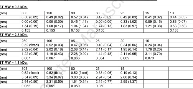
Table 2. ARXPS curve fit parameters and parameter as a function of PST MW and film thickness.
PST MW = 0.8 kDa.
d (nm) 300 150 90 80 25 15 10
b 0.50 (0.02) 0.49 (0.02) 0.52 (0.04) 0.47 (0.02) 0.42 (0.03) 0.41 (0.02) 0.44 (0.03)
(nm) 0.00 (0.00) 0.00 (0.00) 0.45 (1.11) 0.00 (0.00) 0.33 (1.02) 0.89 (0.15) 0.86 (0.07) (nm) 1.54 (0.19) 1.60 (0.17) 1.04 (1.34) 1.74 (0.13) 1.83 (0.97) 1.21 (0.38) 0.53 (0.58)
0.155 0.153 0.158 0.150 0.133
PST MW = 2.5 kDa.
d (nm) 260 105 95 25 20 15
b 0.52 (fixed) 0.52 (0.03) 0.47 (0.05) 0.40 (0.04) 0.34 (0.06) 0.24 (0.04)
(nm) 2.02 (0.04) 2.02 (0.18) 2.08 (0.14) 2.11 (0.17) 1.95 (0.14) 1.76 (0.20) (nm) 1.22 (0.25) 1.19 (0.43) 2.28 (0.92) 1.44 (0.48) 2.11 (0.95) 3.11 (0.70)
0.067 0.067 0.066 0.064 0.065 0.070
PST MW = 4.1 kDa.
d (nm) 305 100 80 25 15
b 0.52 (fixed) 0.52 (fixed) 0.52 (fixed) 0.38 (0.06) 0.19 (0.13)
(nm) 3.54 (0.09) 3.34 (0.07) 3.00 (0.06) 2.94 (0.34) 2.86 (0.34) (nm) 2.94 (0.50) 2.31 (0.50) 1.61 (0.34) 2.15 (0.77) 2.95 (1.37)
0.052 0.051 0.050 0.050
Accepted Manuscript
Figure 1. C 1s spectra at = 90o. a) PST. b) PVEE.
a)
b)
x 104
0 2 4 6 8 10 12
In
te
ns
ity
300 298 296 294 292 290 288 286 284 282 280 Binding Energy (eV)
x 103
0 2 4 6 8 10 12 14 16 18
In
te
ns
ity
Accepted Manuscript
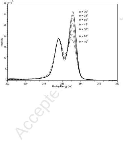
Figure 2. Angle resolved C 1s spectra for a PST(4.1 kDa) / PVEE(3.8 kDa) blend film ~ 305 nm thick.
x 103
0 5 10 15 20 25 30 35
In
te
ns
ity
292 290 288 286 284 282 280
Binding Energy (eV)
= 90o
= 60o
= 30o
= 20o = 10o = 75o
Accepted Manuscript
Figure 3. C 1s curve fit for a PST(4.1 kDa) / PVEE(3.8 kDa) blend film ~ 305 nm thick, =
90o.
x 103
5 10 15 20 25 30 35
In
te
ns
ity
292 290 288 286 284 282 280
Accepted Manuscript
Figure 4. A hyperbolic tangent CDP.
50 60 70 80 90 100
0 2 4 6 8 10
f
(z
)
%
b
Accepted Manuscript
Figure 5. Angle resolved profiles for PST(0.8 kDa) / PVEE(3.8 kDa), blend films. a) Experimental points and least squares fit lines. b) Hyperbolic tangent CDPs corresponding to a).
a) b) 55 60 65 70 75 80 85 90 95 100
1 2 3 4 5 6 7 8 9 10 11 12
3lsinq (nm)
f (q ) P V E E %
300, 80,
25,20, 10nm
0 10 20 30 40 50 60 70 80 90 100
0 2 4 6 8 10
z (nm) f (z ) P V E E
[image:27.595.57.541.171.740.2]Accepted Manuscript
Figure 6. Angle resolved profiles for PST(2.5 kDa) / PVEE(3.8 kDa), blend films. a) Experimental points and least squares fit lines. b) Hyperbolic tangent CDPs corresponding to a).
a) b) 55 60 65 70 75 80 85 90 95 100
1 2 3 4 5 6 7 8 9 10 11 12
3lsinq (nm)
f (q ) P V E E %
260, 105,95 nm
25 nm 20 nm 15 nm 0 10 20 30 40 50 60 70 80 90 100
0 2 4 6 8 10
f (z ) P V E E %
260, 105 nm
20 nm
15 nm
[image:28.595.54.543.171.747.2]Accepted Manuscript
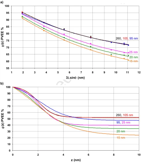
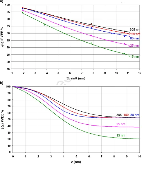
Figure 7. Angle resolved profiles for PST(4.1 kDa) / PVEE(3.8 kDa), blend films. a) Experimental points and least squares fit lines. b) Hyperbolic tangent CDPs corresponding to a).
a) b) 55 60 65 70 75 80 85 90 95 100
1 2 3 4 5 6 7 8 9 10 11 12
3lsinq (nm)
f (q ) P V E E
% 305 nm
100 nm 80 nm 25 nm 15 nm 0 10 20 30 40 50 60 70 80 90 100
0 1 2 3 4 5 6 7 8 9 10
f (z ) P V E E %
305, 100,80 nm
25 nm
[image:29.595.55.544.174.757.2]Accepted Manuscript
Figure 8. SFM topography images. a) PST(0.8 kDa) / PVEE(3.8 kDa). b) PST(289 kDa) / PVEE(3.8 kDa).
a) b)
Vertical scale = 30 nm. Vertical scale = 60 nm.
Film thickness ~ 90 nm. Film thickness ~ 120 nm.