This is a repository copy of
Value-Based Manufacturing Optimisation in Serverless Clouds
for Industry 4.0
.
White Rose Research Online URL for this paper:
http://eprints.whiterose.ac.uk/130540/
Version: Accepted Version
Proceedings Paper:
Dziurzanski, Piotr orcid.org/0000-0001-9542-652X, Swan, Jerry and Soares Indrusiak,
Leandro orcid.org/0000-0002-9938-2920 (Accepted: 2018) Value-Based Manufacturing
Optimisation in Serverless Clouds for Industry 4.0. In: Proceedings of the Genetic and
Evolutionary Computation Conference. The Genetic and Evolutionary Computation
Conference, 15-19 Jul 2018 . (In Press)
[email protected]
https://eprints.whiterose.ac.uk/
Reuse
This article is distributed under the terms of the Creative Commons Attribution (CC BY) licence. This licence
allows you to distribute, remix, tweak, and build upon the work, even commercially, as long as you credit the
authors for the original work. More information and the full terms of the licence here:
https://creativecommons.org/licenses/
Takedown
If you consider content in White Rose Research Online to be in breach of UK law, please notify us by
Value-Based Manufacturing Optimisation
in Serverless Clouds for Industry 4.0
Piotr Dziurzanski
Department of Computer Science,University of York York, UK
Jerry Swan
Department of Computer Science, University of York
York, UK [email protected]
Leandro Soares Indrusiak
Department of Computer Science,University of York York, UK
ABSTRACT
There is increasing impetus towards ‘Industry 4.0‘, a recently pro-posed roadmap for process automation across a broad spectrum of manufacturing industries. The proposed approach uses Evolu-tionary Computation to optimise real-world metrics. Features of the proposed approach are that it is generic (i.e. applicable across multiple problem domains) and decentralised, i.e. hosted remotely from the physical system upon which it operates. In particular, by virtue of beingserverless, the project goal is that computation can be performed ‘just in time’ in a scalable fashion. We describe a case study for value-based optimisation, applicable to a wide range of manufacturing processes. In particular, value is expressed in terms of Overall Equipment Efectiveness (OEE), grounded in monetary units. We propose a novel online stopping condition that takes into account the predicted utility of further computational efort. We apply this method to scheduling problems in the(max,+)algebra,
and compare against a baseline stopping criterion with no predic-tion mechanism. Near optimal proit is obtained by the proposed approach, across multiple problem instances.
CCS CONCEPTS
·Computer systems organization→Cloud computing; ·
Ap-plied computing→Supply chain management; ·
Comput-ing methodologies→Genetic algorithms;
KEYWORDS
Plant optimisation, Genetic Algorithm, Value Curve, Stopping Con-dition, Function as a Service, FaaS, Serverless Clouds.
1
INTRODUCTION
The ‘Industry 4.0‘ concept1envisions increasingly automated man-ufacturing, characterized by the integration of Computational In-telligence methods into the production process. Properties typi-cally associated with Industry 4.0 include a) interoperability of the cyber-physical components of the system and b) decentralized decision-making. Widespread adoption of Industry 4.0 will clearly not be possible if the Computational Intelligence methods require signiicant bespoke efort. The proposed methods must therefore exhibit both a high degree of cross-domain genericity and also require minimal end-user expertise to be applied to some variant application domain. Relative to other optimisation methods, these are both advantages enjoyed by Evolutionary Computation.
In this article, we present a case study of a distributed ‘Function as a Servce’ (FaaS) system that uses Evolutionary Computation
1http:⁄⁄www.plattform-i40.de⁄I40⁄Navigation⁄DE⁄Home⁄home.html
to perform scalable optimisation. We address a real-world issue that is frequently neglected in many traditional benchmarks: the efect that time spent optimising has on overall manufacturing proit (OEE). We present a novel stopping condition which takes this into account. We deine a model that combines manufacturing proit⁄loss with the predicted value of further computation. To obtain both genericity and real-world grounding, combined model values are expressed in terms of monetary units (sometimes termed ‘$EE’ instead of OEE [17]).
The central notion of Industry 4.0 is that, by being rapidly re-sponsive to the dynamic arrival of manufacturing orders, customers can then require only several units of a highly customised product [6]. They will have a set of highly conigurable machines with au-tomated material handling systems and a cloud-based management system [3]. Such a service-oriented manufacturing model will also aim to maximise the proit from the plant by sharing manufacturing resources across a number of manufacturing orders [15].
An ubiquitous optimisation problem in smart factories is the allocation of manufacturing resources over time, while satisfying constraints in terms of time and cost [15]. But even a single ma-chine can be conigured in multiple ways, depending on the re-quired manufacturing schedule (priorities, delivery time, etc) and sustainability constraints (consumables and⁄or energy-saving con-ditions) [4]. Hence, optimisation is naturally interleaved with the manufacturing process in an online manner. This motivates the pro-posed approach of scalable optimisation with a grounded stopping criterion.
resources are needed on demand, cloud based optimisation using Genetic Algorithms (GA) is proposed in this paper. Evolutionary algorithms have been shown to be particularly efective in such applications [5] and performing the optimisation process in clouds can decrease the related costs [16]. To reduce the optimisation cost even further, theFunction as a Service (FaaS)serverless cloud com-puting model has been chosen. Using this architecture, customers not only do not have to maintain the computing infrastructure, but are billed for the actual execution time of the computing resources, which are expected to become available within milliseconds of request. Thanks to these properties, the proposed optimisation scheme can be highly scalable depending on the size of the optimi-sation problem and timing constraints. Each of these possibilities is investigated in this paper.
Contribution:We propose a new modeling technique for
man-ufacturing orders. This technique beneits from (i) thea priori
knowledge of the dynamic value stemming from completion of the optimisation process at certain time, (ii) predicted utility of further optimisation, (iii) scalable computing resources available on demand in the serverless cloud computing architecture.
It is typical in optimisation research for the trade-of between solution quality and execution time to be implicit, with the latter often being expressed in terms of a coarse measure such as ‘number of evaluations of the objective function’. This is of course good scientiic practice, but is not suicient to capture the needs of our real-world application. The second contribution therefore employs a value curve to make this trade-of completely explicit, grounding computational processing in terms of monetary proit, as described earlier.
2
RELATED WORK
In this Section, we discuss previous work related the three com-bined aspects of this paper: i) GA stopping criteria, ii) value-based heuristics, iii) evolutionary optimisation in the cloud:
Stopping Criteria
According to Michalewicz [19], the most common stopping cri-teria of a GA are either a) statically-determined upper limits on the number of generations or itness function evaluations or b) dynamic prediction of further improvement based on genotypic and⁄or phenotypic convergence. Safe et al [21] argue that dynamic prediction is preferable. One of such alternatives has been proposed by Hernandez et al [12], with an adaptive stopping criterion which was experimentally shown to stop at optimal solutions with a high probability. In Hajji et al [10], a stopping criterion based on an approximation of the objective function has been compared with criteria based on both genotypic and phenotypic convergence. The genotypic convergence was evaluated by comparing the percentage convergence of each gene against a certain threshold. The phenotyp-ic convergence was evaluated using two metrphenotyp-ics:online performance
converges to a stable value when the solutions converge andoline performanceconverges when the probability of improving the so-lution decreases. The approximation-based method gave the best results of the proposed approaches, but at the expense of greatest computation time. The online and oline performances were much faster and close to the approximation-based ones with regard to
quality. The genotypic criteria were shown to be not eicient. Con-sequently, in our proposed approach only phenotypic convergence is considered.
In Yin et al [29], the Standard Deviation (SD) of itness values is employed as a stopping criterion, terminating the optimisation process when SD is lower than a given threshold. In that paper, an SD-based stopping criterion has been shown to speed up the con-vergence and shorten the search time for scheduling independent tasks in a grid environment. This criterion is also used as a part of our proposed stopping criterion.
Perroni et al focus on an estimation of a beneicial stopping point for any swarm-based search algorithm [20]. In that paper, a sequence of auto-adapted exponential and log-like curves are proposed to model the algorithm convergence. In this paper, a similar approach based on the rational function extrapolation [25] is used to predict future itness values and thus apply a value-based heuristic to trade between the potential value gain due to a better solution quality and the loss caused by the longer computation.
Value Based Heuristics
The main goal of value-based heuristics is to inform a decision process that maximises overall value to end-user [1]. Several value-based heuristics have been employed to allocate processing tasks. Theocharides et al [27] assumed task values to be ixed, whearas Burns et al [2] allow task values to change over time. In the lat-ter case, the value can be described with a so-calledvalue curve, a function whose domain represents the computation time (with origin at the release time of the process⁄container), whereas the codomain represents the values themselves [13]. Typically, a value curve is non-increasing and reaches a value of zero at a certain time point. After that point, there is no beneit from computing the task and it can be dropped to avoid consuming unnecessary processor resource. During each scheduling event, a task with the highest value at that moment can be selected, as discussed in Theocharides et al. The innate risk of such technique is to select a task with large outlying resource requirements, where a set of less computation-ally expensive tasks may actucomputation-ally be preferable. Burkimsher et al [1] proposed to irst allocate tasks with maximal remaining value, calculated as the area under the value curve from the current time to the zero point. A number of value-related heuristics have been compared by Singh et al [24], highlighting the beneits originating from the access to historic execution data. In this paper, a similar assumption is made: the estimated execution time of a GA invoca-tion (termed a ‘stage’, hereafter), based on historically measured cases, is used to decide whether to terminate stage sequencing.
Value-based allocation of Docker containers have been proposed by Dziurzanski et al [8]. However, the authors of that paper focused on allocation of multiple independent containers to maximise the cumulative value, whereas the goal of this paper is to maximise the proit obtained from a single manufacturing order. Moreover, the related execution cost was not considered in that paper. Similarly, containers were executed in a local cluster, with customised sched-uler installed on each node, whereas we instead focus on execution using serverless clouds.
A complementary notion to the value curve, entitled ‘price curve’, has been used in Henzinger et al [11] to present a varied cost of
GA-based optimisation in a serverless cloud Optimisation
order
Prediction of further revenue
improvement
negative
positive
Solution
Figure 1: General scheme of the proposed approach
computing resources. In contrast, we assume constant cost for executing an optimisation engine in a cloud, as this is case for the major cloud vendors. We share with Henzinger the expression of value curves in monetary units.
Cloud-based Evolutionary Computation
A recent position paper [22] presents a conceptual worklow for the deployment and execution of distributed GAs. The software container technology (Docker) and a lightweight Linux distribution created to execute containers (CoreOS) has been used for large and scalable deployments on diferent infrastructure, focusing on secu-rity, consistency and reliability. This idea has been further extended in Salza et al [23], where evolutionary machine learning classiiers have been deployed to the cloud. In the proposed solution, a similar architecture is used for performing evolutionary optimisation. In particular, Docker containers are used to execute instances of jMet-al[7], a popular Java framework ofering a variety of algorithms for single- and multi-objective metaheuristic optimisation.
In Ma et al [16], a master-slave topology implementing a dis-tributed evolution algorithm was employed. The master assigned the individuals from each generation to the slave nodes based on their load information and then collected the corresponding itness values. The comparison with allocation of the same number of in-dividuals to each node has been conducted for 32, 48 and 64 nodes. The obtained improvement of the computation time has ranged from 6% to 39% depending on the cluster size. While shortest time was achieved for the largest case, the strategy proposed in that paper has not considered heterogeneous architecture or various communication costs. The proposed solution also takes communica-tion overhead into consideracommunica-tion. Since our approach is serverless, the number of nodes is decided dynamically.
Leclerc et al [14] propose a cloud-based framework facilitating large scale evolutionary experiments. Their framework provides a master-slave architecture, with nodes communicating via JSON over HTTP. The applied scheduling policy aims to uniformly spread the load across peers. The slave node with minimal load is chosen for each incoming itness function evaluation task. There is no possibility of sharing processing units between tasks. Consequently, if there is no slave with an idle processing unit, the task is placed in a FIFO queue. To guarantee the appropriate amount of computing resources, the framework is intended to be executed on virtual machines (VMs) whose number is steered by the cloud provider, using facilities such as Amazon Auto Scaling Group. When the smoothed expected time to empty the queue is larger or smaller than certain thresholds, a VM is added or removed, respectively.
In contrast, in an approach advocated by a recent position pa-per [26], the framework presented in this papa-per executes a GA
1
2
5
6
3
4
A C F
D
[image:4.612.56.293.86.139.2]B E
Figure 2: Activity on Arrow representation of a plant
on several machines in accordance with theserverlesscomputing paradigm. The motivation for the serverless approach is to provide both scalability and cost-efectiveness: payment is made only for actual computation performed.
From this literature survey, it follows that there is no prior work on stopping criteria for maximizing increase the overall beneits of an optimization process that is itself costly. This problem is investigated in this paper, the general scheme of which is illustrated in Fig. 1.
3
SYSTEM ARCHITECTURE AND PROBLEM
DESCRIPTION
The class of optimisation problems analysed in this paper concern manufacturing plants. The value gained by an end-user from the optimisation depends on both solution quality and the time taken by the optimisation process itself. Since the optimisation process is performed by a serverless cloud, the system architecture covers the problem domain model and the cloud coniguration.
In the following, we further describe the two components of Fig. 1. For the considered case study, the left-hand component corresponds to the optimisation of manufacturing plant that is speciied via the(max,+)algebra. In the right-hand component,
the stopping criterion is applied to the iterated application of the optimisation process in order to maximise overall proit.
3.1
Plant Optimisation
The plant model used in this paper is based onmax-plus algebra, a discrete algebraic system in which themaxoperation takes the role of addition (⊕) and the traditional addition operator instead takes on the role of multiplication (⊗). The max-plus algebra is convenient for modeling discrete event systems, since the basic operations of such systems, such as temporal transitions and synchronisation, can be described with a set of simple linear equations [9].
A simple example of a plant is presented in Fig. 2 using the ‘Activity On Arrow’ (AOA) notation. In this notation, the states (1, . . . ,6in Fig. 2) represent synchronisation points whereas the actual manufacturing activities (a.k.a. processes) are performed on traversal between states via arrows (A, . . . ,Fin Fig. 2). In this example, a manufacturing process begins at timet1in state1. The
irst manufacturing process is performed during transitionA be-tween states1and2, which lasts fordAtime units. Thus, state2 is visited att2 =t1⊗dA =t1+dA. Similarly,t3 =t2⊗dB and
t4=t3⊗dD. The production process represented by arrowFcan start after bothCandEare completed, so the max operator is ap-plied,t5 =(t2⊗dC) ⊕ (t4⊗dE). Finally, the last manufacturing process, represented by arrowF, is inished att6=t5⊗dF.
Inpractice, the processing time in each manufacturing process is not constant, as machines can operate in variousmodes[4], for examplefull performanceorecomodes. The optimisation process then includes not only the assignment of jobs to machines, but also the selection of the mode that minimises production cost, there-by inding a compromise between processing time and dissipated energy.
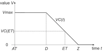
As discused above, in the considered optimisation problems, both solution quality and optimisation time are relevant to the end-user. The value stemming from the later is described by a value curve V C[2, 13]. This curve is expressed in a monetary unit (e.g. GBP). A value curve is usually a monotonically decreasing function. Its highest value equals toVmaxfrom the manufacturing order arrival up to the deadline of the manufacturing order scheduling. Then it trends towards zero with the increasing completion time due to penalty, for example as shown in Fig. 3, where the value curve V Cof manufacturing orderOassumes its maximal value from the arrival time ofO,AT, to the deadline of the optimisation ofO,D. The optimisation time of manufacturing orderOlasts fromATto ET. The total income of an end-user depends partially on the value of the value curve atET.
The reduction in the manufacturing order value due to delay can be determined by observing the value of the value curve at the delayed completion time. A long optimisation time may result in zero value and thus the job becomes worthless to its end-user. Further, the cost of this optimisation can be considered as a loss. Therefore, the manufacturing order may be rejected if zero or a negative value is expected after completing it.
3.1.1 GA encoding, operators and fitness.The underlying opti-misation problem considered in this case study is the coniguration of a manufacturing process, speciied by thesequencingof a ixed number ofmachines, each with a ixed number ofoperating modes. The corresponding geneome is therefore an integer-based represen-tation, derived from the structure of the AoA network representing the plant, e.g. as shown in Fig. 2. The genome consists of a sequence of pairs(m,o)for machinemand operating modeo. There is one such pair for each arrow in the corresponding AoA representation. The chosen GA operators are the familiar random mutation, one-point crossover and selection, with mutation probability0.01
and crossover probability of0.7, these values being obtained after a
small amount of manual tuning. The population size has been ixed to 500 in all the experiments.
The itness of a coniguration is given as a weighted sum of the
makespanandenergydissipated, each of which are a function of both machine placement in the AoA graph and the associated mode of each machine. It has the same monetary unit as the given value curveV Cof the optimised problem.
3.2
Prediction of Revenue Improvement
The optimisation is performed during a number of stages. During thei-th stagei∈ {1, . . .n}, GA iterations are executed in parallel.
Then the results are gathered and a stopping condition is checked, based on the prediction of the total value improvement in the sub-sequent stage.
We now describe the parameterisation of the case study consid-ered in this paper.
time t
value V
AT D
0
ET
Vmax
VC(t)
VC(ET)
[image:5.612.353.525.83.168.2]Z
Figure 3: An example value curve of manufacturing orderO
Table 1: Symbols and abbreviations used in the paper
Symbol Description
O manufacturing order
V C value curve
AT manufacturing order arrival time
D manufacturing order optimisation deadline
Z manufacturing order zero value time
Vmax maximal value of the manufacturing order value curve
fi minimal itness function value after thei-th stage
ˆ
fi a predicted value offi
β cost of a container execution per time unit (constant)
pi no. of containers executed during thei-th stage
ti time of computing of thei-th stage (measured)
ci cost of computing thei-th stage
Ti cumulative time of computing the irstistages
Ci cumulative cost of computing the irstistages
Pi proit generated after computing thei-th stage
ˆ
Pi prediction ofPi
ˆ
ti prediction ofti
ˆ
ci prediction ofci
Ii income obtained after thei-th stage
sdi standard deviation of the population after stagei
3.2.1 Problem parameters.Symbols and abbreviations used are summarised in full in Table 1. Each problem instance is parame-terised as follows:
• Input: manufacturing orderOincluding: the plant given in the AoA form, its value curveV Cand arrival timeAT, a po-tentially unbounded number of slave processing nodes with (monetary) execution cost per time unitβand the number of individuals sent to each processing node.
• Objective: Maximise the proit obtained from the
manufac-turing order.
The proit from the manufacturing order depends on the follow-ing factors:
• the itness value returned by the GA,
• total processing time allocated to the optimisers, • cloud processing cost (per container invocation).
4
PROPOSED APPROACH
We now proceed to describe the proposed approach.
4.1
Value curve
The value curve models the value of a process to its end-user as a function of time,V C(t). It may assume various shapes, as discussed in Burkimsher [1]. For the proposed approach, the shape shown in Fig. 3 has been chosen, which models generating the maximum
value (e.g. as agreed in a contract) up to a certain deadline, after which a certain penalty is imposed every time unit. This shape can be intuitively explained as up to the deadline, the factory is occu-pied with other, previously conigured manufacturing orders. So the deadline is the earliest time the factory can start manufacturing new products. Thus, there is no extra beneit in computing a new coniguration well before the deadline, but after the deadline the factory becomes idle until a new coniguration is found. As during this idle interval both relative overhead cost (ROC) and relative direct labor cost (RDLC) are incurred proportional to the idle time, the value of the solution decreases [17]. Without any further mod-iication of the proposed approach, this shape can be exchanged with any other non-increasing function if a curve better describing a certain process is identiied.
The chosen value curve assumes positive values starting from the time of the manufacturing order arrival,AT. As in this paper we consider only a single order scenario, without any loss of generality it may be assumed thatAT = 0. The maximum value ofV C(t) is equal toVmax and is observed fromAT to a certain deadline,
D>AT. Finally,V C(t)assumes zero value from zero value time,
Z >D. This shape of the value curve can be described with the following equation
V C(t)=
Vmax forAT <t ≤D,
−Vma x
Z−D (t−D)+Vmax forD<t ≤Z,
0 fort>Z.
(1)
4.2
Time and cost of stage execution
The optimisation is performed in stages until the applied stopping condition is satisied. The stage index is denoted withi,i ∈ N.
During thei-stage, the optimisation is performed onpi slave nodes. As these nodes are executed in the FaaS manner, the monetary cost of using them is given by valueβper second for each instance (for example, in IBM Cloud it was $0.000017 per second of execution, per GB of memory allocated on 21.01.2018). The maximal slave execution time in thei-th stage is equal toti. Thus the upper-bound on cost of the execution of this stage for containerciis given by:
ci =β·ti·pi. (2)
The cumulative cost of computing the irstiiterations,Ci, is equal to:
Ci =
i
Õ
j=1
cj. (3)
The predicted execution time of a stage,tˆiis determined via the extrapolation mechanism described in Section 4.3. The manufactur-ing income yielded after thei-th iteration is a diference between the income given by value curveVTat the moment of completion thei-th stage and the manufacturing cost, described by itness value fi, i.e.
Ii =V C(Ti) −fi. (4)
The proit generated after execution of thei-th stage is expressed as a diference between the income and the cumulative cost of the optimisation:
Pi=Ii−Ci. (5)
4.3
Value prediction
The values ofti and fi can be predicted via extrapolation. The extrapolation method used is the Bluirsch and Stoer algorithm [25], an extension of the well-known Neville interpolation⁄extrapolation algorithm todiagonalrational functionsp(x)/q(x)for polynomials p,qwherepis of degreem(the length of the history vector from
which to extrapolate) and the diagonal property requires thatqis of degreemorm+1, according asmis even. In many cases, this
method can be analytically shown to provide superior accuracy to more traditional methods of polynomial extrapolation [25]. For history lengths of 3 or less, such extrapolation is either undeined or else the result was empirically determined to be inaccurate: the predicted value offi is then given by the best itness found so far and that oftiby the last (actual) processing time. After predicting the valuesfˆi,tˆi, they are used to predict the proit generated after the subsequent,(i+1)-th stage as follows:
ˆ
Pi+1=V C(Ti+tˆi+1) −fˆi+1−Cn−cˆi+1. (6)
This value can be used in a value-based stopping criterion, as described in the subsection below.
4.4
Stopping criteria
The stopping criteria are evaluated for a container at each stagei. We irst apply anabsolutecriterion (ensuring that the process will eventually terminate) by comparing theito a ixed upper bound on the number of stages (here, a value of 100 was empirically cho-sen). Thephenotypic convergencecriterion compares the Standard Deviationsdi of the GA population against a threshold value (here, 0.02), similarly to e.g. Yin et al [29]. Thepredicted proitcriterion uses the method of diagonal rational extrapolation described above to predict whether the execution of the subsequent stage will not decrease the proit generated by the optimised process or not:
Pn >Pˆn+1. (7)
The beneits of these stopping criteria are evaluated in Section 6.
5
IMPLEMENTATION ISSUES
Similarly to Leclerc et al [14], the proposed optimisation process is implemented using a master-slave paradigm: the master is ex-ecuted locally and awaits manufacturing orders. Upon arrival of a manufacturing order, its role is to prepare an appropriate plan-t coniguraplan-tion scheme and generaplan-te a seplan-t of individuals for plan-the GA-based optimisation. This data is sent to a certain number of slave nodes, where, at each stage, the actual GA-based optimisation algorithm is executed for a certain number of iterations. Finally, the results are returned to the master node which evaluates the stopping condition as described earlier in this paper.
The GA-based optimiser, executed remotely by the slave nodes,
has been implemented within thejMetalframework and placed
inside a Docker container [18]. This container acts as a REST-compliant Web service, awaiting input in the form of a population of proposed plant conigurations (i.e. manufacturing worklows) to be optimised. After performing the stipulated number of GA iterations (see Section 6), the container returns a new generation of proposed plant conigurations. Communication between the master and slave nodes is performed via JSON over HTTP.
As previously mentioned, since the slave nodes are stateless, they are not bound to a particular optimisation process and thus can be executed in accordance with the serverless computing paradigm. This means that the slave nodes are executed on demand without provisioning virtual machines. Slave nodes do not have to be active between consecutive invocations and thus the company is billed only for the real computation time of the slaves. One of the public vendors that ofer ‘on demand’ execution of a Docker container is
IBM OpenWhisk2. When an OpenWhisk Docker action is invoked
by the master via a REST API call, OpenWhisk pulls the Docker image for the slave node from Docker Hub and then forwards the input HTTP POST request with the coniguration and individuals. After inishing the computation, the request responds with the resulting population of conigurations and the slave node is killed. Alternatively, Apache OpenWhisk3can be also used in a private cloud or a public cloud provided by other vendors.
6
EXPERIMENTAL RESULTS
To evaluate the proposed optimisation approach, we irst describe the application to a single large manufacturing plant. We then consider a larger number of problem instances.
6.1
A larger problem instance in-depth
The selected plant is representative of the larger instance sizes encountered when the system is coupled to the real-world equip-ment of the project’s industrial partners. It is described by an AoA instance with 22 nodes, 6 levels and 43 arrows. Each manufactur-ing process can be executed usmanufactur-ing one of 8 machine types, each having from 1 to 9 operating modes with diferent performance and energy dissipation. The manufacturing cost depends on the selected machines and their modes, as described earlier. The search space for such an instance is too large to be realistically solvable by exhaustive methods without incurring overall monetary loss due to increased optimisation time.
The value curve given for this particular instance is consistent
with equation (1), with assumed parametersAT = 0,D =500s,
Z = 1000s,Vmax = 5000GBP. One second of computations is
assumed to costβ =0.5GBP (lower values of this parameter are
applied later in this section) and the initial number of containers run in parallel is set top1=10. In each stage, a ixed number of
generations of a GA is executed.
As described above, the followingbaselinedynamic stopping
criteria are applied to each container: (i) the Standard Deviation of population itness after theith stage,sdi ≤10−6or(ii) minimal itness function valuefi was not improved during the previous 20 stagesor(iii) the number of stagesi =100, used as a guarantee for the computation ending. The proposed criteria difers from this baseline by the additional inclusion of proit prediction.
During execution, criterion (i) stopped the continuation in a certain container after the 34th stage for the irst time. So, after this stage, 9 parallel containers continued the execution (i.e.p35=9)
up to stage 46th, where another container stopped computation and so on. Finally, as many as 71 stages have been computed and
2https:⁄⁄console.bluemix.net⁄openwhisk⁄
3https:⁄⁄openwhisk.apache.org⁄
-4000 -3000 -2000 -1000 0 1000 2000 3000 4000
1 5 10 15 20 25 30 35 40 45 50 55 60 65 70
Pr
of
it
[G
B
P]
[image:7.612.342.525.86.201.2]Stage
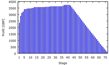
Figure 4: Proit yielded after each stage of the example plant
with computation costβ= 0.5GBP
0 500 1000 1500 2000 2500 3000 3500 4000
1 5 10 15 20 25 30 35 40 45 50 55 60 65 70
Pr
of
it
[G
B
P]
Stage
Figure 5: Proit yielded after each stage of the example plant with no computation costs
during the last stage only two containers continue the optimisation process (p71=2).
After eachith stage, the itness function value to be computed in the next (i+1-st) stage is predicted as described in subsection 4.3. The average prediction error was circa 2%. This accurate prediction can be well exploited by the proposed value-based stopping criteria, as discussed later.
The proitPiobtained after ending computation at eachith stage is presented in Fig. 4. The highest proit is obtained after relatively earlyi=5th stage. After this point, due to increasing computation cost and the decreasing slope of the value curve after the 40th stage, the yielded proit is signiicantly lower and beyond the 49th it becomes negative. Clearly, the baseline stopping criterion triggers too late. This is in contrast to the criterion proposed in equation (7). After applying this criterion, the proit is predicted to decrease after the 6th stage, which is the second best during the whole analysed range and only 2% worse than the highest possible proit.
In the previous example, a rather high cost of performing com-putation has been assumed. Let us compare these results with the second extreme case presented in Fig. 5, when the computation is performed for free, i.e.β =0. In this case, the proposed stopping
criterion from equation (7) terminates the execution after the 41st stage, which yields the highest possible proit. After this stage, the proit drops due to the decreasing slope of the associated value curve.
[image:7.612.342.527.259.370.2]0 20 40 60 80 100
100 200 500 0 20 40 60 80 100
Pe
rc
en
ta
ge
o
f
th
e
m
ax
im
um
pr
of
t
[%
]
Ex
ec
uti
on
ti
m
e
[s
]
Generations per stage
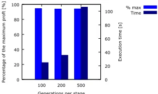
[image:8.612.329.548.82.251.2]% max Time
Figure 6: Proit and execution time obtained for containers executing assorted iteration numbers
6.2
Granularity
Inthis experiment, diferent numbers of GA generations, namely 100, 200 and 500, have been executed at each stage, during each container invocation. The experiment has been conducted for 10 diferent manufacturing orders, with representative characteristics, with the number of required manufacturing processes ranging from 18 to 59. The averaged results are presented in Fig. 6. As it is visible in the graph, the analysed granularity levels have no inluence on the proit yielded by algorithm, as in all three cases it is almost equal to the maximal achievable proit from the given plants. However, the execution times of the considered optimisation processes difer signiicantly as it is more than 4 times longer for 500 generations per stage than 100 generations per stage.
6.3
Scalability
The proposed approach beneits from a serverless cloud execu-tion, so that the number of containers executed in parallel can be easily scaled. The number of containers executed in parallel does not inluence the total computation time, but it increases the total computation cost, as each second of container computation costsβ. Fig. 7 visualises the proit obtained from the optimisation of the plant described in subsection 6.1. In this experiment, various numbers of containers computing in parallel, from 1 to 10, were tested, with computation costs ranging fromβ =0toβ=0.5GBP.
Despite the fact that ‘number of containers’ is discrete, a 3D surface plot has been used to facilitate observation. It is worth noting that theβaxis is expressed in a logarithmic scale (excepting the boundary caseβ = 0), as typical serverless computation cost is
expected to be close to0.00005GBP, but other orders of magnitude are added to cover a wider range of cloud architectures.
From this igure, it follows that the highest proits are yielded in the middle of the analysed range, forpi =4. This value can be then treated as a trade-of between the beneits of parallel execution, i.e. evolving the best results independently by a few optimisation processes and the increased monetary cost by executing a higher number of containers in parallel. But even in case of lower execution costs (including the extreme caseβ =0), no additional proit is
yielded by scalingpibeyond 4.
Since using the larger number of containers increases costs, the higher standard deviation of the yielded proit considering various βhas been observed for the largest number of the containers run in parallelpi = 10. This value decreases almost linearly up to
Figure 7: Computation cost per second by parallelisation
pi =4, for which standard deviation of the yielded proit is almost
10 times lower than forpi =10. So, if no parallelism is applied, the computational costβis less important.
6.4
Stopping criteria
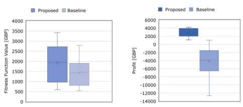
In order to compare the proposed approach with the baseline stop-ping criterion, 30 manufacturing orders whose number of manu-facturing process steps ranged from 18 to 59 have been optimised using both the approaches. The maximal possible income value from each of the manufacturing order is equal to 5000GBP.
The stopping criterion used for baseline comparison does not consider proits: it is triggered when the itness function value has not been improved for a certain number of generations. This is in contrast with the proposed stopping criterion, which aims to maximise proit by stopping the optimisation when no further proit gain is predicted. Consequently, the optimisation of a manu-facturing order is stopped much earlier. For the considered set of manufacturing orders, the optimisation process has been complet-ed 18.5 times faster. Hence, during such signiicantly shorter time, the obtained itness function values are, on average, 34% worse, as shown in the box plot in Fig. 8 left (lower is better). However, the goal of the proposed method is to maximise the proit, which depends both on the itness function value and the computation time. The impact of the latter results in the fact that using the base-line stopping criteria, 86% of the considered manufacturing orders lead to inancial loss, whereas all of them are proitable when the proposed stopping criterion is applied. These proits are shown on the right of Fig. 8 (higher is better). Applying the proposed criterion leads to a cumulative proit of 83877GBP, whereas the baseline cri-terion lead to the negative proit of -124497GBP. Formal statistical comparison of the proposed and baseline proits for each problem instance (pairwise, via the Wilcoxon Signed Rank test) conirms signiicance (withp-value1.9∗10−9).
7
CONCLUSION
This article describes a serverless, cloud-based architecture that provides general and scalable support for the ‘Just in Time’ man-ufacturing process envisioned for ‘Industry 4.0’. The architecture
[image:8.612.91.254.85.182.2]Figure 8: Comparison of the itness function value (left) and proit (right) obtained with the proposed and the baseline stopping criteria
isequipped with a novel adaptive stopping criterion for optimis-ing Overall Equipment Efectiveness (OEE), in which the predicted cost⁄beneit ratio of performing further optimisation is grounded in monetary units. The method was applied to a collection of repre-sentative case studies for optimal coniguration of manufacturing plants, as speciied via the(max,+)algebra. We determined the
most efective parallelisation strategy (implemented via stateless, Dockerised containers) and obtained near maximum proit from the resulting optimisation.
ACKNOWLEDGMENTS
The authors acknowledge the support of the EU H2020 SAFIRE project (Ref. 723634).
REFERENCES
[1] Andrew Burkimsher and Leandro Soares Indrusiak. 2016. Bidding policies for
market-based HPC worklow scheduling.CoRRabs⁄1601.07047 (2016).
[2] Alan Burns, Divya Prasad, Andrea Bondavalli, Felicita Di Giandomenico, Krithi Ramamritham, John Stankovic, and Lorenzo Strigini. 2000. The meaning and role of value in scheduling lexible real-time systems.Journal of systems architecture 46, 4 (2000), 305ś325.
[3] Baotong Chen, Jiafu Wan, Lei Shu, Peng Li, Mithun Mukherjee, and Boxing Yin. 2017. Smart Factory of Industry 4.0: Key Technologies, Application Case, and
Challenges.IEEE Access(2017).
[4] Nancy Diaz, Elena Redelsheimer, and David Dornfeld. 2011. Energy consumption characterization and reduction strategies for milling machine tool use.Glocalized solutions for sustainability in manufacturing(2011), 263ś267.
[5] Ulrich Dorndorf and Erwin Pesch. 1995. Evolution based learning in a job shop scheduling environment.Computers & Operations Research22, 1 (1995), 25ś40. [6] Jocelyn Drolet, Colin L Moodie, and Benoit Montreuil. 1989. Scheduling factories
of the future.Journal of Mechanical Working Technology20 (1989), 183ś194.
[7] Juan J Durillo and Antonio J Nebro. 2011. jMetal: A Java framework for multi-objective optimization.Advances in Engineering Software42, 10 (2011), 760ś771. [8] Piotr Dziurzanski and Leandro Soares Indrusiak. 2018. Value-Based Allocation
of Docker Containers. InThe 26th Euromicro International Conference on Parallel, Distributed, and Network-Based Processing (PDP).
[9] Hiroyuki Goto. 2014. Introduction to max-plus algebra. InProceedings of the 39th International Symposium on Symbolic and Algebraic Computation. ACM, 21ś22.
[10] Omessad Hajji, Stéphane Brisset, and Pascal Brochet. 2003. A stop criterion to accelerate magnetic optimization process using genetic algorithms and inite element analysis.IEEE transactions on magnetics39, 3 (2003), 1297ś1300. [11] Thomas A Henzinger, Anmol V Singh, et al. 2010. A marketplace for cloud
resources. InProceedings of the tenth ACM international conference on Embedded
software. ACM, 1ś8.
[12] German Hernandez, Kenneth Wilder, Fernando Nino, and Julian Garcia. 2005. Towards a self-stopping evolutionary algorithm using coupling from the past. In Proceedings of the 7th annual conference on Genetic and evolutionary computation. ACM, 615ś620.
[13] Bhavesh Khemka, Ryan Friese, et al. 2015. Utility functions and resource
manage-ment in an oversubscribed heterogeneous computing environmanage-ment.IEEE Trans.
Comput.64, 8 (2015), 2394ś2407.
[14] Guillaume Leclerc, Joshua E Auerbach, Giovanni Iacca, and Dario Floreano. 2016.
The seamless peer and cloud evolution framework. InProceedings of the 2016 on
Genetic and Evolutionary Computation Conference. ACM, 821ś828.
[15] Yongkui Liu, Xun Xu, Lin Zhang, Long Wang, and Ray Y Zhong. 2017.
Workload-based multi-task scheduling in cloud manufacturing.Robotics and
Computer-Integrated Manufacturing45 (2017), 3ś20.
[16] Ning Ma, Xiao-Fang Liu, Zhi-Hui Zhan, Jing-Hui Zhong, and Jun Zhang. 2017. Load balance aware distributed diferential evolution for computationally
ex-pensive optimization problems. InGECCO Proceedings Companion, 2017. ACM,
209ś210.
[17] Darin Marcus and Laron Colbert. 2015. $EE, the Financial Aspect of
OEE. (2015). https:⁄⁄www.qualitydigest.com⁄inside⁄operations-article⁄
091715-ee-inancial-aspect-oee.html
[18] Dirk Merkel. 2014. Docker: Lightweight Linux Containers for Consistent
Development and Deployment. Linux J.2014, 239, Article 2 (March 2014).
http:⁄⁄dl.acm.org⁄citation.cfm?id=2600239.2600241
[19] Zbigniew Michalewicz. 2013.Genetic algorithms + data structures = evolution
programs. Springer Science & Business Media.
[20] Peter Frank Perroni, Daniel Weingaertner, and Myriam Regattieri Delgado. 2017. Estimating stop conditions of swarm based stochastic metaheuristic algorithms. InProceedings of the Genetic and Evolutionary Computation Conference. ACM, 43ś50.
[21] Martín Safe, Jessica Carballido, Ignacio Ponzoni, and Nélida Brignole. 2004. On stopping criteria for genetic algorithms.Advances in Artiicial IntelligenceśSBIA 2004(2004), 405ś413.
[22] Pasquale Salza, Filomena Ferrucci, and Federica Sarro. 2016. Develop, Deploy
and Execute Parallel Genetic Algorithms in the Cloud. InGECCO Proceedings
Companion, 2016. ACM, 121ś122.
[23] Pasquale Salza, Erik Hemberg, Filomena Ferrucci, and Una-May O’Reilly. 2017. Towards evolutionary machine learning comparison, competition, and
collabora-tion with a multi-cloud platform. InGECCO Proceedings Companion, 2017. ACM,
1263ś1270.
[24] Amit Kumar Singh, Piotr Dziurzanski, and Leandro Soares Indrusiak. 2015. Value and energy optimizing dynamic resource allocation in many-core HPC systems. In Cloud Computing Technology and Science (CloudCom), 2015 IEEE 7th International Conference on. IEEE, 180ś185.
[25] J. Stoer, R. Bartels, W. Gautschi, R. Bulirsch, and C. Witzgall. 2002.Introduction to Numerical Analysis. Springer New York.
[26] Jerry Swan, Steven Adriaensen, et al. 2015. A Research Agenda for Metaheuris-tic Standardization. InProceedings of the Eleventh Metaheuristics International Conference (MIC), Agadir, Morocco. https:⁄⁄goo.gl⁄kC06p5
[27] Theocharis Theocharides, Maria K Michael, Marios Polycarpou, and Ajit Din-gankar. 2010. Hardware-enabled dynamic resource allocation for manycore
systems using bidding-based system feedback.EURASIP Journal on Embedded
Systems2010 (2010), 3.
[28] Chee Shin Yeo and Rajkumar Buyya. 2006. A taxonomy of market-based resource
management systems for utility-driven cluster computing.Software: Practice and
Experience36, 13 (2006), 1381ś1419.
[29] Hao Yin, Huilin Wu, and Jiliu Zhou. 2007. An improved genetic algorithm with
limited iteration for grid scheduling. InGrid and Cooperative Computing, 2007.
GCC 2007. Sixth International Conference on. IEEE, 221ś227.