University of South Carolina
Scholar Commons
Theses and Dissertations
1-1-2013
Using Singular Value Decomposition in Classics:
Seeking Correlations in Horace, Juvenal and Persius
against the Fragments of Lucilius
Thomas Whidden
University of South Carolina
Follow this and additional works at:https://scholarcommons.sc.edu/etd Part of theComparative Literature Commons
This Open Access Dissertation is brought to you by Scholar Commons. It has been accepted for inclusion in Theses and Dissertations by an authorized administrator of Scholar Commons. For more information, please [email protected].
Recommended Citation
Using Singular Value Decomposition in Classics: Seeking Correlations in Horace, Juvenal and Persius against the fragments of Lucilius
by
Thomas Whidden
Bachelor of Arts
California State University Northridge, 1999
____________________________________
Submitted in Partial Fulfillment of the Requirements
For the Degree of Doctor of Philosophy in
Comparative Literature
College of Arts and Sciences
University of South Carolina
2013
Accepted by:
Paul Allen Miller, Major Professor
Mark Beck, Committee Member
Catherine Castner, Committee Member
Duncan Buell, Committee Member
© Copyright by Thomas Whidden, 2013 All Rights Reserved
DEDICATION
I dedicate this to my beloved wife who smiles and supports me
ACKNOWLEDGEMENTS
First, I would like to express my sincere appreciation to Dr. Beck who
encouraged me many moons ago to actually pursue a degree instead of simply
taking random Greek and Latin courses. I wish to thank Dr. Castner whose love
for Latin and excitement for the Classics was motivational in my desire to know
Latin well. Although Dr. Gardner is not a part of my dissertation committee I have
benefited greatly from not only her storehouse of knowledge, but her kindness in
letting us graduate students develop our own thoughts about a text even when
she knows we are dead wrong. I wish to thank Dr. Sefrin-Weis for her lofty
academic standards to push me to excel. The B+ in Aristotle has not only driven
me to do better, but has kept me humble. Dr. Buell deserves an award for not
only putting up with a hack of a programmer, but he pointed me in the right
direction toward SVD. Without this nudge this dissertation would be sorely
lacking. I would be remiss unless I credit Dr. Miller who saw this dissertation in
its infancy in a shorter paper I wrote for him. His oversight and gracious words of
encouragement were greatly appreciated. Last, I wish to credit my wife with her
ABSTRACT
For the purpose of this dissertation, the hypothesis is posited that a
programmatic correlation of the poems of Lucilius and the other Satirists reveals
a detailed and dense level of intertextuality, especially in those poems which
scholars already understand to allude to the genre's inventor. In addition to those
poems which are discussed in secondary literature, we have discovered other
poems which correlate highly with the corpus of Lucilius, but have been largely
ignored. To demonstrate this fact I have devised a method using Singular Value
Decomposition. That method is able to discern this subtle intertextuality in both
the texts in question as well as other Classical texts since our method is not
language-specific. We have discerned Horace to be the most highly correlated
to Lucilius, and further, poem 1.4 to be among the most highly correlated to
Lucilius' fragments. In the course of writing this dissertation we will examine
other poems which are found to be highly correlated to discover what we
hypothesized--if there is a subtle intertextuality which has been largely ignored.
We will use what I term a "roving correlation" on target poems to pinpoint dense
TABLE OF CONTENTS
DEDICATION...iii
ACKNOWLEDGEMENTS...iv
ABSTRACT...v
LIST OF TABLES...vii
LIST OF FIGURES...x
LIST OF SYMBOLS...xi
LIST OF ABBREVIATIONS...xii
INTRODUCTION...1
CHAPTER 1 - Introduction to Computer Correlation...6
CHAPTER 2 - Our Method...46
CHAPTER 3 - Horace's highest correlated poem to Lucilius...64
CHAPTER 4 - Lucilius Book 26 & Juvenal 9, A Comparative Study ...72
CHAPTER 5 - Situating the Dubious Fragments...100
CHAPTER 6 - Conclusion...109
CHAPTER 7 - Research Tools...115
REFERENCES...117
APPENDIX A - Formulae...131
APPENDIX B - Word Lists for Subject Correlations...134
APPENDIX C - Stop Words...141
APPENDIX D - All Coefficients of H, P and J against L...142
APPENDIX E - Pearson Coefficients of Moby Dick...180
APPENDIX F - Unassigned Fragments Coefficients...181
APPENDIX G - Unassigned Fragments from xxvi-xxix...186
APPENDIX H - Math Sanity Check...189
LIST OF TABLES
Table 1.1 Example document vectors/document matrix...27
Table 1.2 Example pangram coefficient correlations...30
Table 1.3 Example pangram coefficient correlations with dogs...31
Table 1.4 Call me Israel coefficients...32
Table 1.5 Negative correlation...34
Table 1.6 Negative correlation document matrix...34
Table 1.7 Skewed correlation...37
Table 1.8 Bad Cosine Similarity example...38
Table 1.9 SVD simple example - unprocessed document matrix...41
Table 1.10SVD simple example - Σ...42
Table 1.11SVD simple example - U...43
Table 1.12 SVD simple example - VT...43
Table 1.13 SVD example - simple pangram document matrix...44
Table 1.14SVD example - simple pangram after SVD...45
Table 2.1 Poe document matrix...48
Table 2.2 Poe document matrix index=3...48
Table 2.3 Pauline coefficient correlations using Galatians...50
Table 2.4 Pauline coefficient correlations using Galatians...52
Table 2.5 Roman Satire corpus correlations...53
Table 2.7 Subject correlations: Proper names...54
Table 2.8 Subject correlations: Animals...54
Table 2.9 Subject correlations: Disease...55
Table 2.10 Subject correlations: Excess...55
Table 2.11 Subject correlations: Food...55
Table 2.12 Subject correlations: Speech...55
Table 2.13 Subject correlations: The body...56
Table 2.14 Subject correlations: The dishonorable...56
Table 2.15 Subject correlations: The gods...56
Table 2.16 Subject correlations: War language...56
Table 2.17 Subject correlations: Women...57
Table 2.18 Subject correlations: Man & virtue...57
Table 3.1 Book 26 against individual poems...64
Table 3.2 Book 27 against individual poems...66
Table 3.3 Book 28 against individual poems...67
Table 3.4 Book 29 against individual poems...68
Table 3.5 Book 30 against individual poems...70
Table 4.1 Personal pronouns in Roman Satire...77
Table 5.1 Dubious fragment coefficients (lines 981-999)...100
Table 5.2 Dubious fragment coefficients (lines 974-980)...101
Table 5.3 Largest fragments in Lucilius...102
Table 5.4 Similar words in fragment 811 and Book 15...103
Table 5.5 Fragment ID 811 against Book 15 (Rank-11)...106
Table 6.1 Proposed metrical document correlation...113
LIST OF FIGURES
Figure 1.1 Schafer and Ernesti's concordance.̈ ...12
Figure 1.2 Packard's concordance...12
Figure 1.3 Entry 1 for ut from Schafer and Ernesti's concordance.̈ ...13
Figure 1.4 Entry 2 for ut from Schafer and Ernesti's concordance.̈ ...13
Figure 1.5 Pearson plot examples...28
Figure 1.6 Intersection of dataset...29
Figure 1.7 Cosine Similarity in 2-dimensional space...29
Figure 1.8 Plot of bad Cosine Similarity...38
Figure 1.9 Plot of bad Cosine Similarity 2...39
LIST OF SYMBOLS
T indicates the transposing of a matrix
Σ indicates summation
LIST OF ABBREVIATIONS
J...Juvenal
H...Horace
P...Persius
L...Lucilius
Introduction
For the purpose of this dissertation, the hypothesis is posited that a
programmatic correlation of the poems of Lucilius and the other Satirists reveals
a detailed and dense level of intertextuality, especially in those poems that
scholars already understand to allude to the genre's inventor. In addition to those
poems that are discussed in secondary literature, we have discovered other
poems that correlate highly with the corpus of Lucilius, but have been largely
ignored. To demonstrate this fact I have devised a method using the known
"Singular Value Decomposition algorithm." That method is able to discern this
subtle intertextuality in both the texts in question as well as Greek texts since our
method is not language-specific. In the course of writing this dissertation we will
examine other poems that are found to be highly correlated to discover what we
hypothesized, if there is a subtle intertextuality that has been largely ignored. We
will use what I term a "roving correlation" (explained below in Chapter 2) on the
target poems to pinpoint dense intertextual areas.
In chapter one we introduce digital documents and computer correlations.
For the purpose of recognizing the significance of not only the technology of
digitizing documents, but the pioneers who were themselves classicists (Roberto
Busa and David Packard), a thorough introduction is needed. When one
recognizes the profound impact digital documents hold and that every web page
great debt. Since the first two digital works were both Latin, the digitizing of
documents has a history based wholly in classical literature.
While these digital documents allowed complete concordances to be
easily made, this blazed a trail for further technological advances. One eventual
advance is the correlation of documents. A computer correlation is an automatic
similarity test using two or more sets of data. We reduce the digital documents in
question to sets of data in order to test their similarity. A direct result of pioneers
like Busa and Packard who created concordances of Latin works led to further
projects in this field discussed below. These projects currently revolutionize how
we work today, and also how we learn.
A document correlation of classical texts would be impossible if not for the
advances in math in the last two hundred years. A discussion of correlating data
would be incomplete without mentioning the inventors of these foundational
mathematical methods. Pearson and Galton not only bestowed upon us
algebraic gifts, but Pearson makes us acutely aware that correlations can be
misleading and therefore we need to be vigilant in interpreting our data. We
introduce various methods for comparing documents and then we demonstrate
these algorithms in a few simple examples. These simple examples show us the
differences and weaknesses of the algorithms introduced and therefore those we
should use for our data. We introduce Singular Value Decomposition that looks
promising in correlating our documents. We settle upon this algorithm for the
basis of our method.
In chapter two we introduce our method. We use the texts of the Roman
necessary words ignoring certain common words so that we do not correlate
texts based upon insignificant words such as conjunctions, pronouns, etc.
(Appendix C). We also create lists of words specific to Roman satire that we use
to do specific correlations upon the satirists. We have marked all proper names
within the satirists in order to do special proper name correlations. These lists
are found in Appendix B. Finally, we prove our method is accurate in identifying
similar texts by taking St. Jerome's Latin translation of the Bible to show the
Pauline books cluster together. We then use our method to correlate the entire
worksof each satirist against one another. We use our special satire subject lists
against each author as well. We demonstrate that ancient and modern
scholarship has shown Horace and Satire 1.4 to be the most similar to Lucilius.
It is no secret that Horace, Juvenal and Persius all refer to the inventor of their
satiric genre, Lucilius. Scholars did not have to make this connection, it was
Quintilian, who first comments on the genre of Satire. Quintilian says Lucilius
achieved high renown by some, but Horace is "much more polished and pure
(10.1.94)." In turn, Horace praises Lucilius as Satire's progenitor. Quintilian says
"Satura quidem tota nostra est," "Satire is entirely ours [Roman] (10.1.93; Miller,
Latin Verse Satire 1)." He cites specifically what Horace says about the style of
Lucilius' poems, that they were "a muddy flow out of which you would want to
take parts." This is a reference to Horace's Satire 1.4.11. Out of the entire genre
of satire, it is significant that Quintilian quotes this lone poem to exemplify both
the genre and its inventor. Our method confirms Horace to be the highest satirist
correlated to Lucilius.
highest correlated poems against the books of Lucilius. Since we have
confirmed what scholarship has seen with Horace 1.4, we can use these data to
find another poem that is highly correlated and do a comparative study on it.
This poem should have a dense intertextuality.
In chapter four we perform a comparative study on Juvenal Satire 9 and
book 26 of Lucilius. We could have used any number of poems from our dataset.
The poem in question for the study was selected randomly. We begin with a
survey of the scholarship that has been done on Juvenal 9 as well as any
scholarship that has compared the Satires of Juvenal with those of Lucilius. We
determine that this comparative study is unique since scholarship has largely
ignored correlating these two texts together. We examine the similarities
between both satirists. There is a similar dialectic in each author as well as
many didactic aspects. Both also display a negative view of marriage. There are
strikingly similar references to Homer. In addition, Lucilius mixes Greek with
Latin throughout his Satires and Juvenal does this as well in his ninth Satire.
This exhibits an extremely close likeness to Lucilius. Last, we explore common
subjects to Roman satire in each of the documents such as crudeness, sexuality
and commerce.
In chapter five we attempt to situate the dubious fragments of Lucilius.
There are fragments of Lucilius that are not assigned to any particular book. In
as much as we can determine intertextuality accurately, we will also be able to
predict to which book the unassigned and dubious fragments of Lucilius belong.
We first try to situate unassigned fragments that are known to belong to a subset
conjecture to situate lines 1196-1208 into book 15 based upon our data and offer
an intertextual justification.
In chapter six we conclude by noting the gaps in our data as well as
offering suggestions for further research. Finally in chapter seven we describe
the tools that have been created in the writing of this dissertation and how they
can be used for further research. It is our hope these tools will not only be useful
Chapter 1 - Introduction to Computer Correlation
Given the interdisciplinary nature of this dissertation a thorough introduction
to the computer processing of documents is à propos. Without this introduction,
the true nature of this dissertation would be impenetrable to the average
comparativist or classicist; therefore, some preliminary remarks are necessary.
We introduce two areas first because modern document correlation is the
product of two independent research ancestries: the history of creating
documents in digital form and the history of using mathematical methods to
measure similarity. Last, we will demonstrate a few simple examples.
Digital Documents
The process of correlating documents using a computer first starts at
digitizing them. A particular document has to be read by a computer in an
organized fashion. Instrumental figures like Roberto Busa and David Packard
were first to conceive and implement electronic texts in order to create
exhaustive concordances. These concordances of Livy and Aquinas are
impressive given the rudimentary computer languages of the time as well as the
slow nature and memory restrictions on their hardware.
David W. Packard's concordance of Livy that was completed in 1968 was a
technologically ground-breaking work, not only because it was one of the first
concordances generated by a computer, but because it was the first work to be
long hours in the space of one year by David Packard, who programmed this
concordance while at Harvard. These hours were shared by those who spent
time typing the text of Livy onto punchcards. One hundred years before David
Packard typed the first word of Livy's text onto punchcards, the necessary
advances in math and computers had begun. David Packard's work opened the
way for other Classical engineering projects.
Oftentimes technology is taken for granted. The Internet is a prime
example. If a website lacks a site search (an area that allows a user to search a
website for a particular word), the site could be seen as primitive. In like manner,
a complete and exhaustive concordance for every work is nowadays a basic
necessity. Furthermore, most books that are printed today can be purchased in
digital format; this makes them easily searched. With resources like
Perseus.org, it is difficult for younger minds to fathom a time when Roman and
Greek works lacked an online searchable database, let alone a complete and
exhaustive physical concordance. This was the predicament in 1960.
Today there are a variety of programming languages that are powerful,
incredibly intuitive and robust in internal functions (Computer). There are many
different open source and commercial database systems that make creating
indexed works effortless. The most remarkable advances though, that were
made, were done so in computer hardware and architecture itself. The speed
and storage space today, compared to the sixties, is profound. Handheld phones
used today have far more storage and CPU power than could be packed into a
computer that took up 1,400 square feet in 1960 (an IBM 701). The cost of one
percent (compare an iPhone at $500 with an IBM 701 that shipped in 1953 at
$1,027,000, Thelen).
It is precisely because the technology in the sixties was so primitive, and
because using computers to process classical works was so new, that
Packard's concordance was such a monumental feat. At the same time, Packard
was being carried on the shoulders of giants with the technology of his day.
Punchcard machines, although seen as primitive today, were a wonder.
The punchcard, or the Hollerith card, was named for Herman Hollerith who first
conceived the idea to store data on a punchcard that could be read by a machine
in 1896 (Punchcard). The original punchcard had been around since 1725
(Punchcard). This card would endure as a reliable storage medium until the
early eighties of the 20th century. These cards were used for data storage, and
even storage for computer programs. They were stacked in piles of 2000 and
read by card readers that would then make their data available to computers.
With the advent of the computer in the early forties, there were men who
immediately understood the ramifications of using these machines to manipulate
large amounts of data (Computer). Roberto Busa was the first to conceive the
idea of creating a concordance with the help of a computer (Winter 4). This
Jesuit priest started planning a concordance for the works of Thomas Aquinas in
1946 (Winter 5). This was quite a task as the works of Aquinas exceeded
10,000,000 words. In 1951 he published a work that showed his proof of concept
and blazed a trail for others to follow in the ensuing decades (Winter 7). Busa
used hand-written punchcards for a single entry of the preposition in (in order to
one entry of many in his 56 volumes (Winter 6). It would be 20 years before
Busa was done typing the works of Aquinas onto punchcards, and 30 years until
this voluminous work was finished (Winter 4).
Inspired by Roberto Busa, John Ellison saw the power of what the
computer could accomplish. He, Remington Rand, Inc. and a Univac I computer
produced a concordance to the Revised Standard Version of the Bible in 1957.
This took only a fraction of the time that James Strong took to complete his
concordance by hand (Ellison Preface) in the 19th century. Although Roberto
Busa is not mentioned specifically in the preface of this Biblical concordance, it is
obvious that Busa's contribution to humanities laid the foundation for this work
(Winter 4). Ellison used punch tape (almost identical to punchcards, but a
continuous strip of paper) that was then transferred to magnetic-tape (Winter 4;
Ellison Preface). This is basically the same process that David Packard would
use a decade later to generate his own concordance. It is to be noted that
technologically at this time, conventional typesetting had to be used. In other
words, his computer-generated concordance still needed to be fed into a
typesetting machine that would have been a great expense and a hindrance to
any humanities departments.
Nothing has been said yet of the advances in computer languages. The
concordances mentioned thus far that were conceived by Ellison and Busa, were
programmed not by Ellison and Busa themselves, but by professional computer
"scientists." I believe one of the reasons why Packard's concordance was
completed so quickly was because he was the only programmer on the task;
Remington Rand, Inc, or IBM (Packard, A Concordance to Livy: Vol I-IV vii). It is
because of the advances in computer languages that David Packard was able to
pick up programming for this project even though his primary training was in
Classics (Packard, A Concordance to Livy: Vol I-IV vii). Although I am unsure of
the language in which Packard programmed (whether FORTRAN, SNOBOL or
Assembly), I am sure of two things. First, in 1968, because of the advances
making programming more intuitive, David Packard could take on this task of
generating a concordance to Livy. And yet, at the same time, comparing the
languages available to Packard to the computer languages today, it would have
been an insanely tedious process to program an index to any text, let alone Latin,
in SNOBOL, FORTRAN, or Assembly language. If Packard had used SNOBOL
rather than FORTRAN, his task of creating a concordance would have been less
tedious since SNOBOL made it easier to handle strings. All this technology was
necessary for David Packard's concordance, both the computer hardware and
also the software. The pioneer work by men like Busa and Ellison set the stage
for David Packard.
Busa chose Thomas Aquinas because his own dissertation in 1946 was
based upon these works. Ellison chose the Bible because he was a man
passionate about the Word of God, but why did David Packard choose Livy?
David Packard was studying Classics at Harvard. No doubt, his passion
for Classics was profound. This is obvious because the decades after he
published his concordance, so much of his time was spent with Greek and
Roman works. He would obviously gravitate to a Classical work for this
software to transfer the text to magnetic-tape (Glickman and Gerrit 1-7), would
have been an incredibly arduous task. He would have had to encode a Greek
text into the punchcard EBCDIC character set. At this time, the text that could be
typed onto a punchcard was limited to what was on a FORTRAN keyboard. This
would have been capital A through Z, 0 through 9 and some additional characters
(Glickman and Gerrit 24). Further, a Roman work had to be selected that could
have been completed within a small time frame since Packard was a fellow for
only a year at the Harvard Computing Center. Even though originally Livy was
142 books, in 1968 and to date, we only have 35 books and books 41 and 43 are
incomplete (Gould x). One has to wonder if Livy would have been chosen if we
had retained all 142 books. It might have taken 3 additional years, or even
longer, to type the text onto punch cards. The number of cards would have been
multiplied by 4. The number of additional concordance volumes would have
easily been 16 with all 142 books. But, as we have only retained 35 books, Livy
was small enough to be completed in one year. One last constraint would have
been typesetting concerns. It would have been difficult to render the Greek text if
one were chosen in place of Livy. One would need to reconfigure the Photon
901 (the typesetting machine Packard used to print his concordance) with a new
character set unless he romanized the Greek text. This machine was limited to
only 288 characters at a time (Packard, "Publishing Scholarly Compilations by
Computer" 75).
Another reason why Livy was chosen was that it serves as a good
introduction to all Roman literature. Since Livy, as Gould declares, is a poet
contrivances, what better author to use as the first computer-generated Roman
work (Gould xi,xii)? One final reason why Livy was probably chosen was that the
only concordance in existence for Livy was the concordance edited by George
Olms, and originally published in 1804 by Schafer and Ernesti. Surely this work̈
took great skill and scholarship to produce without the aid of computers. And this
concordance would have been helpful to scholars from 1804 down to the
present. But when you compare this concordance to David Packard's
concordance, it is sorely obsolete.
Compare this entry from Schafer and Ernesti's concordance to that of̈
Packard's concordance.
Figure 1.1 Schafer and Ernesti's concordance.̈
Figure 1.2 Packard's concordance.
While both excerpts have the four entries that exist in Livy, Packard's
concordance is easier to read and contains more context before and after the
source entry. Furthermore, when we examine a given word with many more
occurrences like the common Latin word ut, there is almost no comparison. Here
Figure 1.3 Entry 1 for ut from Schafer and Ernesti's concordance.̈
Schafer and Ernest chose no more than 35 entries to display from the entirë
corpus of Livy. This is understandable since the work is only a small single
volume. Compare this to Packard's concordance that has every entry for ut. It
comprises 47 pages. Packard arranges his concordance entries for every word
with subsequent words in alphabetical order so that similar constructions can be
easily viewed. This would be helpful for any scholar looking at Livy's use of
similar ut constructions. Additionally, the font is so antiquated in Schafer and̈
Ernest that it is almost unreadable. The references in this old concordance are
also difficult to view because they are not lined up. Packard's concordance lines
up all entries so that they can be read easily.
Unlike the concordances of Ellison and Busa, David Packard gave us a
summary of the process of his concordance, not only in the concordance itself,
but in subsequent journal articles. I believe it was this forethought that inspired
Humanities departments all over the world to travel along the trail Busa, Ellison
and now Packard blazed.
While Packard's work seems like trailblazing through terra incognita, the
University of Toronto put out a manual to create concordances of literary works
by computers in 1966. In this manual, they outline programs already written in
FORTRAN that were specifically for scholars who have no previous knowledge of
programming. There are 3 PRORA (Programs for Research On Roman
Authors). PRORA I is to transfer a literary text that has been typed out in a
certain format on punchcards to magnetic tape, PRORA II prints the text in a
certain format, and PRORA III actually creates a rudimentary concordance, or
concordances that were created before David Packard's concordance are not
mentioned in other computer concordance histories, we have to wonder whether
David Packard knew about the research at the University of Toronto. It sounds
as though this manual and its corresponding programs (if the University of
Toronto would have shared these programs) could have made the work that
Packard did infinitely easier.
At any rate, the process that Packard used was not unlike Ellison and
Busa. Packard and some others who were attached to Harvard took turns typing
out the Oxford classical text of Livy for the first 25 books. After that, the Teubner
edition for the remaining 10 books was used. The entire work of Livy took 65,000
punchcards, as it is approximately 505,000 words. This is about 7.8 words per
punchcard. When you remember the punchcard machine limitations in
characters it will become obvious that conventional typing is not the same as
what they had to produce. They would have needed to encode the text
somewhat. Brutus alio ratus spectare Pythicam vocem (Gould 88) would need to
become, *BRUTUS ALIO RATUS SPECTARE *PYTHICAM VOCEM. Asterisks
would need to denote capital letters since all text would be in capital letters.
This would add a layer of complexity to the proofing of the text. Additionally,
some convention to denote book, chapter and verse would have been needed as
well that would create even more noise when proofing the text (Glickman and
Gerrit 29).
After the text was completely typed out, these 65,000 punchcards that
would have been treated as Vatican-like relics were each proof-read. One
any computer today, and another would read through the Latin text of Livy. When
an error in the punchcard was found, the reading would stop and the offending
punchcard or punchcards would be fixed. The old punchcards would then be
discarded. This was done through the entire 35 books of Livy (Packard, A
Concordance to Livy: Vol I-IV vi).
After this first proofing, the 65,000 cards were fed into a card reader
attached to an IBM 7094 with magetic tape storage. The cards were read 2000
at a time and a program ran that placed the text of Livy onto magnetic tape. An
additional program built an index at this time using the text of Livy and listing
every unique word with its references in the entire work of Livy. This is very
similar to what the University of Toronto's manual outlines (Glickman and Gerrit
14). It is to be noted that there were no database servers in 1968. Any
processing of the text by Packard had to be done manually through a program
and stored in some sort of flat text file. This would have been the bulk of the
heavy lifting of the concordance. It would have been a feat to do this in any
computer language that was around in 1968. Even using a string-friendly
language like SNOBOL, Packard would have had to write much logic to create
the index in preparation for his concordance. Many languages today are even
more conducive to processing text than what would have been available in 1968
(Packard, A Concordance to Livy: Vol I-IV vi).
After this index is built another proofing would have been done. They read
through each unique word to eliminate erroneous words generated by the index
program. It is at this time as well, another program was written to cycle through
magnetic tape. Another program as well did a Latin spell check for errors not
found during the other proofing stages. Again all this code had to be done from
scratch by David Packard. He indicates in his preface that the programming of
this concordance took many hours, and often it was done on an irregular
schedule to the chagrin of his wife, whom he thanks for her devotion during this
time (Packard, A Concordance to Livy: Vol I-IV vi).
One last reading aloud was done through the entire text of Livy to find any
residual errors. After this last proofing, the program ran that built the actual
concordance from the index. Packard mentions that the runtime to build the
actual concordance was 3 hours. The concordance to Livy was completed albeit
electronically. It existed although only on magnetic tape. They could have
printed directly onto an IBM peripheral printer and published it in that form. The
typeset would have been abominable and at some point when technology caught
up, the concordance would surely have been reprinted. Instead of using a
default printer, and because of the costs that would have been involved in
conventional typesetting, Packard used a typesetting machine that was able to
read the magnetic tape of his concordance attached to the IBM 7094. He
mentions that he had to write an additional program in order to print his
concordance on the Photon 901 typesetting machine. Essentially, he had to
program his own printer driver to finish his concordance. The output from the
program that processed his concordance occupied 50 reel to reel tapes, or
eleven miles of tape, that is, 133 megabytes (Packard A Concordance to Livy:
Vol I-IV vi; Packard, "Publishing Scholarly Compilations by Computer" 75). A one
storage. Last, Packard mentions that he also created other study tools with the
work on magnetic tape, but it was beyond the scope of the concordance
(Packard, A Concordance to Livy: Vol I-IV vii). It seems at the end of his project,
he saw the benefit and potential for even more processing of the text.
Packard's work endures to this day as a useful reference work, and the
definitive concordance for the body of Livy's text. It has not been supplanted by
another work because it is extremely functional. Aside from the actual
concordance, though, because of Packard's work, other departments benefited
from his ingenuity in lowering typesetting costs. He inspired other humanities
departments to use computer technology in the processing of text. And it also
paved the way for other technological projects in the ensuing decades.
First, because Packard's concordance was not supplanted by any other
concordance, every work that concerned Livy after 1968 has probably benefited
directly from this concordance. It would be unthinkable to write anything on Livy
without consulting this exhaustive concordance. Greenaugh in his Commentary
on Livy Books I and II, that was published in 1976, as well as Gould and Whiteley
in their updated edition of Livy Book I, published in 1987, no doubt used
Packard's concordance to check their own references in their respective prefaces
(Gould, xiv,xv; Greenaugh xiv-xvii). In their commentaries, they could easily
cross-reference similar clauses to give greater insight to the users of their
editions. In addition to these works, any scholarship in Livy would benefit from
the use of this concordance.
With the use of the Photon 901, Packard opened the door to other
even for works that are not computer-generated. Any large work that would need
to be printed could be typed and sent to a computerized photo typesetting
machine. It would obviously have been a huge expense to purchase one of
these typesetting machines, but as it could be used for any department, it would
swiftly pay for itself. We know Packard's work helped lower costs by his use of
typesetting at Harvard and with the Loeb Classical Library years later (Crane).
Finally, Packard's work inspired not only himself for a lifetime of the digital
processing of classics, but also motivated other humanities departments to get
involved as well. Directly after Packard finished his concordance, he started
working on the groundwork of digitizing texts for his Ibycus project. With the
Ibycus environment, David Packard modified the Hewlett Packard minicomputer
for the optimization of searching digital works (Crane). This environment was
purchased by many classics departments all over the world. Although this
environment was tailored for classicists, Crane says this project not only inspired
the creation of the Thesaurus Linguae Graecae, but also influenced their choice
of architecture and environment (Crane). David Packard's work also gave
Oakman more practical knowledge of computer generated concordances with
which to make his recommendations in his manual for building concordances
with computers at the University of South Carolina (Oakman 412,413). His work
also inspired Howard-Hill to sift through all the various types of approaching
computer concordances, and educate any prospective researchers in the area of
digital concordances (Howard-Hill 1-4). Scores of other projects had as their
inspiration Busa and Packard in the ensuing decades including Lexicon of Greek
a project of Oxford University); The Gutenberg Project (purports to have created
eBooks in 1971 and seeks to further digitize all books in the public domain); The
Perseus Project (established in 1985 to allow the reading of Greek and Latin
texts online by Tufts University); Thesaurus Linguae Graecae (established in
1972 to digitize for search all Greek literature from antiquity to the present as a
project of the University of California, Irvine); Suda On Line: Byzantine
Lexicography (established in 1998 to produce XML-encoded database files of
texts); The Digital Medievalist (established in 2003 to digitize medieval texts as a
project of the University of Lethbridge); The Homer Multitext Project (established
in 2006 as a project of Harvard University to use digital media to show textual
variants not simply in a critical apparatus, but more as an alternate performance
of the same story in Homer); Sermones.net (established in 2007 to digitize
medieval Latin sermons); Google Books (established in its infancy in 2002, it
partners with libraries and book producers in order to create the largest
searchable online library); et al. (Bodard and O'Donnell).
Mathematical Methods to Compare Similarity
The history of using mathematical principles to compare data/documents is
more than a hundred years old. These principles are used today as "scientists
use bayesian filters to decide if 'this model is better than the alternatives
(Hobson, Jaffe, Liddle, Mukherjee and Parkinson 3).'" In Bayesian Methods in
Cosmology, correlations are used in order to identify extremely remote objects in
space. Mathematical methods are used to compare similarity when a Google
search is performed, or when Google's news articles are viewed. These news
order to group them together. What is astounding is that the formulae used in
these searches that we perform every day were originally created and
implemented without the aid of calculators or computers. Just as the reformation
is succinctly summed up in the quote "Erasmus laid the egg that Luther hatched,"
it could equally be said of correlation that Galton laid the foundation, but Pearson
built the edifice (Porter 250). "Francis Galton invented correlation, but Karl
Pearson was chiefly responsible for its development and promotion as a scientific
concept of universal significance (Aldrich 364)".
Francis Galton is often remembered not as a pioneer in the field of
correlation or statistics, but for his work in the field of fingerprints. He was
instrumental among others, such as Faulds, Herschel, Henry and Bertillon, in
justifying fingerprints as a reliable method of identification of criminals to Scotland
Yard (Forrest 210,220). While Francis Galton was originally a geographer and
meteorologist, it was not until later in life, when he turned his gaze toward the
study of heredity, that he made his most powerful contribution (Forrest ix). This
contribution proved most fruitful not only for his pupils and peers, but for
generations onward.
The seeds of Galton's interest in heredity came about early in his marriage
and while at Cambridge. As he rubbed shoulders with England's elite he noticed
that talent could be traced throughout generations.
I have no patience with the hypothesis occasionally expressed, and
often implied, especially in tales written to teach children to be
good, that babies are born pretty much alike, and that the sole
and man are steady application and moral effort. It is in the most
unqualified manner that I object to pretensions of natural equality.
The experiences of the nursery, the school, the university and of
professional careers are a chain of proofs to the contrary (Forrest
89).
Galton saw inequality in the abilities of men: some had better cognitive ability
such as memory capacity or mathematical reasoning (Forrest 89). Later when
he married Louisa, who was unable to conceive during her life, he noticed that
infertility could be seen among members of her family (Forrest 85). This caused
him to speculate that her own infertility was genetic. A decade earlier Quetelet
had argued that Scottish chest sizes of soldiers fell along a Gaussian curve or
bell curve (developed by De Moivre in 1733), that is "the law of deviating from an
average." Galton argues this can apply to other features of the human body,
cognitive ability and all other genetic traits (Forrest 89, 90).
Galton dedicated himself to anthropometry no doubt being influenced by his
half-cousin Charles Darwin's seminal work in the animal kingdom. Galton
comments on this book that influenced his own research.
The publication in 1859 of the Origin of Species by Charles Darwin
made a marked epoch in my own mental development, as it did in
that of human thought generally. Its effect was to demolish a
multitude of dogmatic barriers by a single stroke, and to arouse a
spirit of rebellion against all ancient authorities whose positive and
(Forrest 84).
Much as Darwin compares primates to humans in skeletal structure, Galton
begins to measure men in all aspects in order to correlate them along an
average. He published his first work on heredity, Hereditary Genius. In this book
he groups men and their cognitive abilities into 16 groups.
There is a continuity of mental ability reaching from one knows not
what height, and descending to one can hardly say what depth. I
propose...to range men according to their natural abilities putting
them into classes separated by equal degrees of merit and to show
the relative number of individuals included in the several classes
(Forrest 90).
The top four groups contain four fifths of the entire population that represent the
average cognitive ability (Forrest 91). The groups that fall above average
cognition grow smaller in population as their cognition increases because the
more talented are rarer. Finally in his X group he groups those one out of a
million who is labeled illustrius. The group just below illustrius are 248 per million
marked as eminent (Forrest 91). He concludes that this normal distribution of
cognitive ability means that you will find 50,000 idiots and imbeciles out of the
'twenty million inhabitants of England and Wales (Forrest 91). It should be
pointed out that Galton makes errors in the processing of his data, but the
correlation concepts behind this are sound (92).
In Galton's short ten page paper, "Co-relations and their Measurement
contains the first correlation values ever calculated. "This paper contains details
of his technique for calculating the correlation coefficient and presents
coefficients obtained from the measurements of 350 adult males (Forrest 197)."
These coefficients are some of the first correlations ever published. The number
on the left is the coefficient calculated that shows relative similarity in the
measurements among these 350 males. In other words, the closer the number is
to one the more similar the features are in all men. Based upon Galton's
coefficient of men's knee heights and statures (0.90), he could expect future
measurements to be extremely similar.
0.80 Cubit (length of forearm) and stature
0.35 Head length and stature
0.70 Middle finger and stature
0.85 Cubit and middle finger
0.45 Head breadth and head length
0.90 Knee height and stature
0.80 Knee height and cubit
Galton demonstrates in this paper that these concepts of correlation have far
reaching implications for all disciplines of science (Forrest 199); he discovered a
general mathematical method that can be applied to any science in order to
measure similarity between data. Even though Galton seems to foresee how
profound his research will impact future generations, he would be shocked to see
how many disciplines today still use many of his concepts. Pearson, Galton's
pupil, comments on this work:
our scientific ideas has spread is in its permanent influence,
perhaps, the most important of his writings. Formerly the
quantitative scientist could only think in terms of causation, now he
can think also in terms of correlation. This has not only enormously
widened the field in which quantitative and therefore mathematical
methods can be applied, but it has at the same time modified our
philosophy of science and even of life itself (Forrest 197-199).
These comments of Pearson can in no way be understated. Pearson is
instrumental in recognizing that Galton had established a new tool to be used in
science powered by mathematics. While Galton's statistical methods were
recognized as important in and of themselves, Pearson was instrumental in
seeing that this method would be put to immediate use by all branches of
science. Using mathematical methods, scientists could use correlation
coefficients in many disciplines to be given hints (Hobson 1).
Karl Pearson's work in correlation was a life-long process starting in 1891.
"He codified the mathematics of Galton's statistical idea (Porter 258)." His work
is so foundational to modern statistics that he is credited with coining not a few
statistical concepts such as Beta distribution, Chi-squared, the coefficient of
correlation, the coefficient of variation, the histogram, homoscedastic, mode,
standard deviation and sampling distribution among others (David 121,122).
Anyone familiar with statistics and probability would be astounded to know that
virtually two men created this entire discipline. Pearson believed that correlation
change in how research is done (Porter 286). He would admit, of course,
throughout his lifetime of evaluating others' correlative work, that he "found more
and more situations in which correlation analysis was misleading (Aldrich 366)."
Pearson is careful to note that "it is possible to obtain a significant value for a
coefficient of correlation when in reality the two functions are absolutely
uncorrelated (Aldrich 364)." It is this dedication to precision and his religious-like
fervor that makes us owe Pearson an additional debt of gratitude. For if Pearson
had been so cavalier to assume all correlations were valid and always had
probative value, statistical methods could have been laughed off the stage of
science forever.
Basic Correlation Examples
In an effort to understand how document correlation works, we use an
extremely simple test document. The contents of this document are the familiar
English pangram: The quick brown fox jumps over the lazy dog. We wish to
correlate this document against a second document to quantify similarity. The
contents of the second document are the following: The fox jumps over the dog.
We can perform an organic correlation quite quickly on our example and
conclude that both documents are extremely similar since the second document
only eliminates the adjectives. However, let us step through some mathematical
correlations to see their strengths and weaknesses.
We start by counting the frequency of the words in each document that gives
us a simple matrix. A matrix is simply columns and rows of numbers of any size.
Each column corresponds to the frequency of words in a particular document
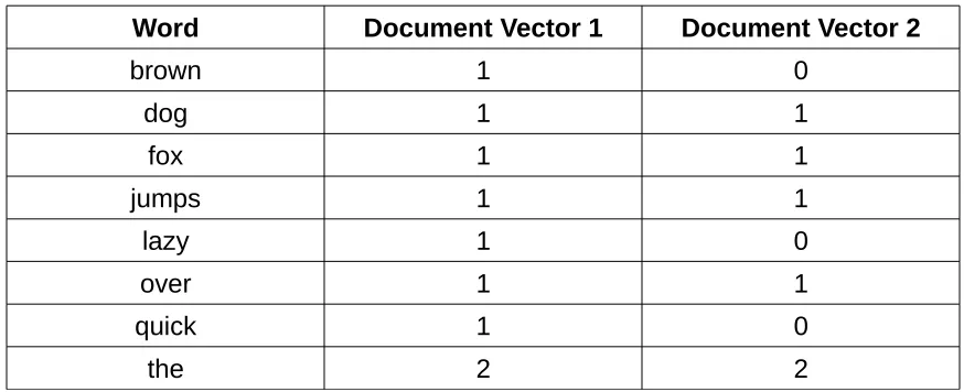
Table 1.1 Example document vectors/matrix
Word Document Vector 1 Document Vector 2
brown 1 0
dog 1 1
fox 1 1
jumps 1 1
lazy 1 0
over 1 1
quick 1 0
the 2 2
We use these document vectors to calculate each of the correlation coefficients.
While we describe all formulae in Appendix A, I believe it is important to
describe these correlations in simple terms in order to understand them. The
matrix above becomes our data points that can be plotted in 2-dimensional
space. These data points are what we will use to calculate similarity using the
various formulae outlined in Appendix A.
Pearson
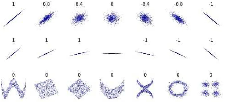
The Pearson correlation that was introduced by Karl Pearson over 100 years ago
is a measure of the linear similarity of a sample data set. The following image
demonstrates sample distributions of data and their respective coefficients
(Pearson Coefficient). The distributions below are document vector data points
Figure 1.5 Pearson plot examples.
As you can see in order to get a positive coefficient there must exist a linear
similarity with a positive slope (a slope that points up to the right).
Jaccard
The Jaccard coefficient is simply the size of the intersection of the data set
divided by the size of the union of the data set. Imagine there are three
document vectors represented by the three circles in figure 1.6 (Jaccard
Coefficient). The intersection of the sample data is demonstrated in A of figure
1.6. The union of all three document vectors is represented by all the letters: A,
Figure 1.6 Intersection of dataset.
The Jaccard difference is simply the Jaccard coefficient minus 1, thus it tells us
simply how far the Jaccard coefficient differs from a perfect similarity indicated by
1.
Cosine Similarity
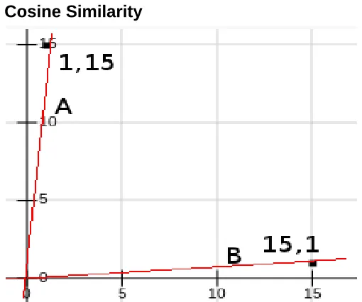
Figure 1.7 Cosine Similarity in two-dimensional space.
Figure 1.7 above is a plot in two-dimensional space. For simplicity sake we only
our plot (0,0). We take the cosine of the angle between these lines and this is
our coefficient.
Tanimoto
Many people use the Tanimoto coefficient as a synonym of the Jaccard index, but
it can be mathematically distinct. This formula reduces our document vector to
zeros and ones. Thus it becomes what is called a bitmap or a bit array (a list of
zeros and ones). In our example a particular document vector has a zero value if
a word does not appear, and a one if a word does appear. For example, if we
have three occurrences of the word dog, the value in our document vector is not
3, but 1. The formula is then the number of common bits between the samples
divided by a set of bits set in either sample, or all samples. Thus if you divide the
common bits (the intersection A above in Figure 1.6) by A, B, C, D, E, F and G,
Tanimoto could become identical to the Jaccard coefficient.
Spearman
Quite simply the Spearman coefficient is the Pearson formula with a twist. The
twist is to rank the values (i.e. the frequencies of words) in ascending order and
then change the respective values before performing the Pearson formula upon
the new values. This process is supposed to get rid of values that are
significantly larger than the rest of the sample. Spearman is then touted to be a
better Pearson in certain circumstances.
Euclidean Dot Product
The Euclidean Dot Product is the sum of the products of individual entries of our
document matrix. For example, if we have a document vector A (1,3,0) and a
respective frequencies of words. These values are then multiplied together
across document vectors and added up: (1 • 2) + (3 • 0) + (0 • 3) = 2. Using this
value we then can calculate the cosine of the angle between our document
vectors: cosθ (where θ represents the angle) = 2 / (square root (12 + 32 + 02) *
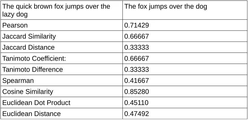
square root(22 + 02 + 32)). Table 1.2 contains all of the coefficients described
above for our simple pangram:
Table 1.2 Example pangram coefficient correlations.
The quick brown fox jumps over the lazy dog
The fox jumps over the dog
Pearson 0.71429
Jaccard Similarity 0.66667
Jaccard Distance 0.33333
Tanimoto Coefficient: 0.66667
Tanimoto Difference 0.33333
Spearman 0.41667
Cosine Similarity 0.85280
Euclidean Dot Product 0.45110
Euclidean Distance 0.47492
For the Pearson coefficient, the Jaccard Similarity, the Tanimoto coefficient and
the Spearman coefficient a value closest to 1 indicates a theoretically perfect
correlation. It is to be noted that these numbers themselves do not indicate an
absolute correlation, but as Pearson said above, they are a hint (Hobson 1). In
other words, the coefficients in question can all be 0.99999 and the data itself
could diverge greatly. We are well-advised by Karl Pearson in his relentless
skepticism of any published correlations. Compare the following table where the
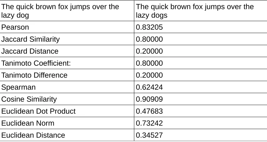
Table 1.3 Example pangram coefficient correlations with dogs.
The quick brown fox jumps over the lazy dog
The quick brown fox jumps over the lazy dogs
Pearson 0.83205
Jaccard Similarity 0.80000
Jaccard Distance 0.20000
Tanimoto Coefficient: 0.80000
Tanimoto Difference 0.20000
Spearman 0.62424
Cosine Similarity 0.90909
Euclidean Dot Product 0.47683
Euclidean Norm 0.73242
Euclidean Distance 0.34527
We would expect a higher correlation given that the documents differ by only 1
word. Perhaps the relatively low coefficients have to do with our small
documents. To illustrate this, we take the first chapter of Moby Dick and change
the two instances of Ishmael to Israel in the second document. Our suspicion is
confirmed with the new coefficients that our test documents were too sparse in
data.
Table 1.4 Call me Israel coefficients.
Call me Ishmael document Call me Israel document
Pearson 0.99996
Jaccard Similarity 0.99540
Jaccard Distance 0.00460
Tanimoto Coefficient: 2.33154
Tanimoto Difference -1.33154
Spearman 0.99216
Euclidean Dot Product 0.56039
Euclidean Distance 0.00686
The Pearson coefficient, the Jaccard Similarity and the Spearman are so close to
1 that their values are almost perfect matches. This confirms that if our data is
sparse, it could yield a relatively low coefficient against a very similar document.
Therefore, low coefficients do not always indicate dissimilar documents. The
Tanimoto Coefficient displayed in Table 1.4 is similar in its calculation to the
Jaccard Similarity (aka Jaccard Index), but it is distinct as described above (See
Appendix A).
Let us compare the first chapter of Moby Dick again to a second document
containing only the first paragraph of this same chapter. For ease of
understanding we calculate only the Pearson Coefficient: 0.80346. This is a
relatively low correlation coefficient. We can change the data slightly to account
for the differing document sizes. We do what is called normalizing the vector
values by adding up all the values of the entire vector, and then divide each
single value by this total. Instead of a clean matrix with whole numbers, our
result is a matrix with decimals. We decide to keep 5 significant digits. Using
this matrix our Pearson coefficient result is not much different: 0.80350. In both
documents there are many words that are insignificant. These words that we
desire to exclude are called stop words. They are words to which we always
assign a zero value so that our calculation knows these words are irrelevant or
too common. For example, if we were correlating two documents with the
content below in Table 1.5, the result (0.85968) would be a relatively high
calculation. We do not want words such as demonstrative pronouns, relative
pronouns, articles, etc.; otherwise they skew our coefficients.
Table 1.5 Negative correlation.
Document 1 Document 2
This is a dog, which is really a canine. This is the pericardium, which is really a membrane.
This is a simple example, but it demonstrates how two documents could be
highly correlated and differ wildly in content. In our calculation, we simply tell the
Pearson algorithm to ignore all words that we deem insignificant: this, is, a,
really, which and the. A decision has to be made whether we want to exclude
these words all together or simply make all their values zero. (A different
coefficient will result depending upon inclusion or exclusion of these zeros.) We
decide to exclude them completely for clarity sake. Our document matrix looks
like the following:
Table 1.6 Negative correlation document matrix.
Word Document 1 Document 2
canine 1 0
dog 1 0
pericardium 0 1
membrane 0 1
Our coefficient in this calculation is -1.00000, a perfect negatively correlated
document, thus absolutely dissimilar. Values can be negative that indicate
conversely, a negatively correlated document, i.e. disimilar documents. Using
compare again the first paragraph to the entire first chapter to see if our result is
any different. Our coefficient becomes 0.60693. While our result is different, the
coefficient in question does not instill confidence in our method. Let us compare
this coefficient against the first paragraph of thirty other random chapters. If our
coefficient is "low," perhaps against other chapters it will seem "high." In fact,
after comparing the first paragraphs of thirty random chapters (see Appendix E),
there is not a single coefficient above 0.07. Our coefficient of 0.60693 becomes
an extremely significant number when juxtaposed against these other
coefficients. Therefore, it is evident that while results can vary wildly, the context
of coefficients is critical. We also need to be mindful to eliminate within the data
itself, that which is insignificant noise.
At this point in our calculations we need to start excluding correlation
coefficient algorithms that do not help us compare documents accurately for our
purposes. As has been stated, we cannot simply assume these formulae are
magic and give us absolute proof as to whether our documents are truly related
or not. This largely depends upon our data, i.e. the documents in question. We
also cannot negate the organic element to correlation. As stated above, Pearson
was mindful of this organic element: false-positives have to be assumed until we
glean evidence to confirm the coefficient in question.
The Jaccard and Tanimoto coefficients are excellent similarity tools. These
particular correlations are still widely used to compare chemical compounds and
genes in molecular biology as well as organic chemistry. We, however, cannot
use them. We exclude them because they both emphasize the presence of
Verducci and Blower 111; Todeschini and Consonni 699). This means that our
use of these correlations depends upon what we are comparing. The absence of
certain words in our documents could equally be significant to those words that
are present. These correlation coefficients do not take this into account, thus we
exclude them.
The coefficient that we have been using for our examples is the Pearson
correlation; this is the flagship of Karl Pearson's life work. It does not suffer from
the problems of the Jaccard and the Tanimoto coefficients, but it does have a
known limitation. "If the data from the rating scale tend to be skewed toward one
end of the distribution, this will attenuate the upper limit of the correlation
coefficient that can be observed. The coefficient can appear inflated in certain
circumstances (Osborne 39)." In other words, if a particular document has an
unduly large frequency of a particular word, the coefficient may result in a high
correlation, but in actuality indicates a high frequency of the single word in
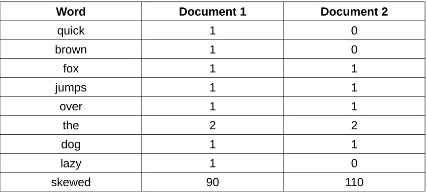
question. A simple example will illustrate these problems. We start with two
documents that compare a simple sentence. The first sentence has adjectives
while the second sentence excludes them. Our Pearson coefficient was
0.71429. We add the word skewed 90 times to the first document and 110 to the
second document. The addition of this single word raises our coefficient to
0.99992. If we change the first document to have 10 instances of skewed and
the second to have only 50, we still end up with a very high coefficient: 0.99932.
The Pearson correlation does not handle these types of documents well. That is,
if your documents have a few data points that are significantly larger than the
these larger numbers (outliers), or weight them differently. For now we exclude
the Pearson correlation.
Table 1.7 Skewed correlation.
Word Document 1 Document 2
quick 1 0
brown 1 0
fox 1 1
jumps 1 1
over 1 1
the 2 2
dog 1 1
lazy 1 0
skewed 90 110
Our next logical step would be to examine the Spearman correlation since it
does not suffer from this problem. Spearman's Rho (Appendix A) is calculated as
0.41667 in our example without outliers and then 0.70909 with both 90/110
instances of the word skewed and with the example of 10/50 instances of the
word skewed. It seems to account for these outliers and gives us a coefficient
that is not too highly correlated. Spearman's rho seems like a great candidate for
our purposes, but an underlying assumption is that your data has a monotonic
relationship (Wikipedia). If the frequency of a given word in document 1
increases, the frequency of that same word never decreases in document 2--this
is a monotonic relationship. Or stated conversely, as the frequency of a given
word in document 1 increases, the frequency of that same word never increases
in document 2. We could not justify such a causal relationship with our data,
The Cosine Similarity is a powerful tool in computing document simlarity. To
illustrate how this coefficient is calculated, take the following simple
two-dimensional document vectors.
Table 1.8 Bad Cosine Similarity example.
Word Document 1 Document 2
puer 1 14
puella 1 14
Here is the corresponding plot of each document vectors.
Figure 1.8 Plot of bad Cosine Similarity.
As you can see the document vectors plotted in two-dimensional space (plotted
from 1,1 and 14,14 respectively) are actually right on top of each other. Normally
you would measure the cosine of the angle from each of these points through the
origin (0,0), but there is no angle to measure that signifies a perfectly correlated
document. The Cosine similarity coefficient in our example has a value of 1, an
ostensibly exact match even though in two-dimensional space they are relatively
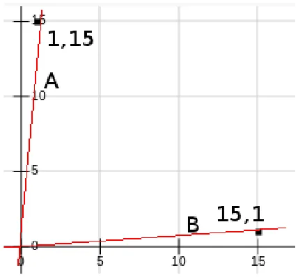
far away from one another. If document 2 had 1 reference to puella and 15
to puer, the plot would look like figure 1.9 below.
Figure 1.9 Plot of bad Cosine Similarity 2.
In such case, we measure the cosine of the angle between line A and line B
through the origin (0,0) that gives us the value 0.13274. This is an extremely low
coefficient, but when compared with our first example, the documents are not all
that different. Both documents mention both target words, but because of their
relation to each other in two-dimensional space one correlates highly, the other
does not. As in our other coefficients, a value close to 1 corresponds to similarity.
Now imagine the vector for document 1 is unchanged (1,1), but for document 2
we change the instances of puer to 100 (1,100). The Cosine coefficient is
0.71414. This is a drastic change by only changing the frequency of one of the
words. In fact, within three examples where all documents have the same words,
we have three very different coefficients. The Cosine similarity is not useless, but
because it does not take into account the magnitude of the vectors (their length),
it is not the wisest choice for our data. The Euclidean Norm also suffers from this
We admit that we could simply run an algorithm to determine outliers and
eliminate them before running a correlation, but we would much rather keep our
document vectors intact. We desire a method that accounts for the entire
document vector without ignoring the absence of words. It also should not
assume an underlying causal relationship between the document vectors.
Singular Value Decomposition may help us in our endeavor to process our matrix
before running a correlation.
Singular Value Decomposition (SVD) was developed by Beltrami and Jordan
in the 1870s and extended later by Golub in the 1960s (Long 161). Many
scientists, mathematicians and scholars describe SVD as a way to simplify a
given matrix (Long 161; Alvo and Ertas 482; Good 823; Hubert, Meulman and
Heiser 69). This simplification exposes the underlying geometric structure, that
allows us to understand better the way the vectors relate to each other. It has
been used over the past 50 years for a variety of applications. It has been used
to correlate areas of the brain (Worsley 915), to classify or organize genes in
organic chemistry (Yeung 6163), to summarize differences in solar radiation that
vary by geographical location (Glasbey 382), image processing (Long 164-166),
to relate genes within DNA studies (Omberg and Golub 18731), to assist in
screening certain patients for different cancer treatments (2052) and in text
processing (Alvo and Ertas 482; Alvarez-Lacalle, Dorow and Eckmann
7956-7959). While it appears to be perplexing to the classicist that an algorithm that
has been so prevalent in scientific studies, can be used to correlate texts, it is
completely natural since we can reduce our texts to a column of numbers, i.e. a