R E S E A R C H
Open Access
The LS-SVM algorithms for boundary value
problems of high-order ordinary differential
equations
Yanfei Lu
1, Qingfei Yin
1, Hongyi Li
1, Hongli Sun
1, Yunlei Yang
1and Muzhou Hou
1**Correspondence:
1School of Mathematics and Statistics, Central South University, Changsha, China
Abstract
This paper introduces the improved LS-SVM algorithms for solving two-point and multi-point boundary value problems of high-order linear and nonlinear ordinary differential equations. To demonstrate the reliability and powerfulness of the improved LS-SVM algorithms, some numerical experiments for third-order,
fourth-order linear and nonlinear ordinary differential equations with two-point and multi-point boundary conditions are performed. The idea can be extended to other complicated ordinary differential equations.
Keywords: Numerical solutions; High-order ordinary differential equations; Two-point boundary value problems; Multi-point boundary value problems; LS-SVM algorithms
1 Introduction
High-order boundary value problems for ordinary differential equations are used to model different problems in some fields such as biology, economics, and engineering. Due to the importance of high-order ordinary differential equations, a considerable size of research work has been carried out about this problem. Among others, finite difference method [1] was proposed to solve two-point boundary value problems for high-order linear and non-linear ordinary differential equations. Homotopy perturbation method [2,3] was used for the solution of fourth-order and sixth-order boundary value problems. Ali [4] proposed the optimal homotopy asymptotic method to solve multi-point boundary value prob-lems. Adomian decomposition method [5–10] was presented for solving two-point and multi-point boundary value problems of high-order ordinary differential equations. Haar wavelets method [11] and Shannon wavelet method [12] were proposed to solve bound-ary value problems of high-order ordinbound-ary differential equations. Doha [13] proposed spectral Galerkin algorithms based on Jacobi polynomials for solving two-point boundary value problems of third-order and fifth-order ordinary differential equations. Doha [14] proposed spectral Galerkin algorithms by using Chebyshev polynomials of the third and fourth kinds for solving high even-order differential equations. Shifted Jacobi collocation method [15] was proposed for solving nonlinear high-order multi-point boundary value problems. Saadatmandi and Dehghan [16] discussed sinc-collocation method for solving multi-point boundary value problems. Variational iteration method [17–19] was applied
to solving two-point boundary value problems of high-order linear and nonlinear ordinary differential equations. Although these numerical methods provide good approximations to the solution, the approximate solution derivatives are discontinuous and can seriously affect the stability of the solution.
Neural network, which is one of machine intelligence techniques, has universal function approximation capabilities [20–22], and the solution obtained from the neural network is differentiable and in closed analytic form. Neural network has been widely used for solving ordinary differential equations [23,24], partial differential equations [25–27], fractional differential equations [28–30], and integro-differential equations [31,32]. Chakraverty and Mall [33] analyzed a regression-based neural network algorithm to solve two-point boundary value problems of fourth-order linear ordinary differential equations. Malek [34] proposed a novel hybrid method based on optimization techniques and feed forward artificial neural networks methods for two-point boundary value problems of fourth-order ordinary differential equations. Mai-Duy [35] discussed radial basis function networks for boundary value problems of high-order ordinary differential equations directly. However, artificial neural network has several drawbacks, such as the need for a large number of con-trolling parameters and the difficult choice of the number of hidden units. Furthermore, its training procedure is time-consuming and can be trapped in local minima.
SVM algorithms [36] were introduced by Vapnik in the framework of statistical learning theory. SVM algorithms map the input data into a high-dimensional feature space using a feature map. SVM algorithms can achieve a global optimum by solving a convex quadratic programming problem. Meanwhile, SVM algorithms adopt the structural risk minimiza-tion principle, which has a better generalizaminimiza-tion performance. LS-SVM algorithms [37] are a modification of SVM algorithms. LS-SVM algorithms change inequality constraints to equality constraints and regard the sum of squared errors loss function as experience loss of the training set. LS-SVM algorithms will deal with a set of linear equations instead of a quadratic optimization problem, which reduces the computation time of model learn-ing significantly and improves higher solution accuracy. Therefore, LS-SVM algorithms have various applications in the area of pattern recognition [38], fault diagnosis [39], and time-series prediction [40,41]. In addition, LS-SVM algorithms have been successfully applied for solving differential equations [42,43], differential algebraic equations [44,45], and integral equations [46].
LS-SVM algorithms are only used to solve two-point boundary value problems of second-order linear ordinary differential equations [42]. To the best of our knowledge, there are not too many results on LS-SVM algorithms for solving two-point and multi-point boundary value problems of high-order linear and nonlinear ordinary differential equations. The main goal of the present thesis is to develop improved LS-SVM algorithms to solve two-point and multi-point boundary value problems of high-order linear and non-linear ordinary differential equations.
efficiency of our proposed LS-SVM algorithms. Finally, concluding remarks are presented in Sect.6.
2 Least squares support vector machines
Consider a given training data set{(xi,yi)|xi∈Rn,yi∈R}Ni=1 (in this papern= 1), where
{xi}Ni=1 are input data points and{yi}Ni=1 are the corresponding output data points. One
assumes that the underlying function describing the relation between input points and output points has the following form:
y(x) =ωTφ(x) +b, (1)
whereωandbare parameters of the model that have to be determined andφ(x) is the nonlinear feature map which maps an input space into a higher dimensional feature space. Then, the optimal solution is sought in that space by minimizing the residual between the model outputs and the measurements [47]. To this end, the LS-SVM model in the primal is formulated as the following optimization problem [37,48]:
min ω,b,ei
J(ω,e) =1 2ω
Tω+1
2γe
Te (2)
subject to
yi=ωTφ(xi) +b+ei, i= 1, 2, . . . ,N,
whereγ is a positive regularization parameter andeiis the error of theith input data. The
first term is a regularization term, while the second one minimizes the training errors. The optimization problem with equality constraints (2) can be solved by using the La-grange multipliers method
L(ω,b,αi,ei) =
1 2ω
Tω+1
2γe
Te– N
i=1
αi
ωTφ(xi) +b+ei–yi
, (3)
whereαi (i= 1, 2, . . . ,N) are Lagrange multipliers that can be positive or negative in the
LS-SVM formulation.
According to the KKT conditions, we will obtain
⎧ ⎪ ⎪ ⎪ ⎪ ⎪ ⎨ ⎪ ⎪ ⎪ ⎪ ⎪ ⎩
∂L ∂ω=ω–
N
i=1αiφ(xi) = 0; ∂L
∂b = N i=1αi= 0; ∂L
∂ei =αi–γei= 0;
∂L ∂αi=ω
Tφ(x
i) +b–yi+ei= 0.
(4)
Whenωandeiare eliminated from a system of Eq. (4), we obtain the following linear
system:
Θij+γ–1E IN–1T
IN–1 0
α
b
=
y
0
whereΘij=K(xi,xj) =φ(xi)Tφ(xj) (i,j= 1, 2, . . . ,N) is theijth entry of the positive definite
kernel matrix;y= [y1,y1, . . . ,yN]T;α= [α1,α1, . . . ,αN]TandIN–1= [1, 1, . . . , 1].
Finally, the LS-SVM model in the dual form can be described as
y(x) =
N
i=1
αiK(xi,x) +b. (6)
3 Brief overview of LS-SVM model for solving ODEs and some definitions In this section, a brief overview of LS-SVM algorithms for solving ordinary differential equations is provided and some definitions are given.
With regard to the initial value problem of the first-order linear ordinary differential equation in the following form [42]:
⎧ ⎨ ⎩ dy
dx=a(x)y(x) +r(x), x∈[a,c],
y(a) =A, (7)
the authors in [42] assume that a general approximate solution isy=ωTφ(x) +b, whereω
andbare the parameters to be solved. Then the interval [a,c] is discretized into a series of collocation points by using collocation methods [49], and the optimal values of the pa-rametersωandbare obtained by solving the optimization problem with constraints, see [42]. According to the Lagrange multipliers method [50], the optimization problem with constraints is transformed into the Lagrangian function which is composed of the LS-SVM cost function and constraints that the approximate solutiony=ωTφ(x) +bsatisfies the given first-order linear ordinary differential equation and the initial condition at the collocation points. The described methodology is applicable for solving other types of dif-ferential equations including second-order boundary value problems, partial differential equations, and descriptor systems [42–44].
The feature mapφ is not explicitly known in general, so the kernel function will be introduced. By utilizing Mercer’s theorem [36], the derivative of the kernel function is defined as [42,44]
∇n,m
K(xi,xj)
=∂
n+m(K(u,v))
∂un∂vm
u=xi,v=xj
=φ(n)(xi)Tφ(m)(xj) = [Θn,m]i,j. (8)
In this paper, the RBF kernelK(u,v) =exp(–(u–v)2/σ2) is considered as a kernel
func-tion, then we can obtain
∇1,3
K(xi,xj)
=∂
4(K(u,v))
∂u∂v3
u=xi,v=xj
=φ(1)(xi)Tφ(3)(xj) = [Θ1,3]i,j
= –
12 σ4 –
12 σ2
2(xi–xj)
σ2 2
+
2(xi–xj)
σ2 4
K(xi,xj);
∇2,3
K(xi,xj)
=∂
5(K(u,v))
∂u2∂v3
u=xi,v=xj
=φ(2)(xi)Tφ(3)(xj) = [Θ2,3]i,j
=
60 σ4 –
20 σ2
2(xi–xj)
σ2 2
+
2(xi–xj)
σ2 4
2(xi–xj)
∇3,3
4 Boundary value problems of high-order ordinary differential equations In this section, we formulate the improved LS-SVM algorithms to the solution of two-point and multi-two-point boundary value problems of high-order linear and nonlinear ordi-nary differential equations.
4.1 Two-point boundary value problems of high-order ordinary differential equations
The improved LS-SVM algorithms to the solution of two-point boundary value problems of high-order linear and nonlinear ordinary differential equations are described.
4.1.1 Nonlinear ordinary differential equations for two-point boundary value problems
Two-point boundary value problems ofMth-order nonlinear ordinary differential equa-tions to be solved can be stated as follows:
dMy
values of the parametersωandbare obtained by the following optimization problem:
subject to
Theorem 1 Given a positive definite kernel function K:R×R→R and a regularization
[Θm,n]2:N–1,2:N–1, [Θ0:S,n1 ]N–2 = [[Θ0:S,n]1,2, [Θ0:S,n]1,3, . . . , [Θ0:S,n]1,N–1] and [Θ0:R,nN ]N–2 =
[[Θ0:R,n]N,2, [Θ0:R,n]N,3, . . . , [Θ0:R,n]N,N–1],m,n= 0, 1, . . . ,M.
Proof Consider the Lagrangian function of the optimization problem (10):
L(ω,yi,αi,ηi,β0,βs,λ0,λr,b,ei,ξi)
Then the KKT optimality conditions are given by
∂L
System (11) is solved by Newton’s method. Therefore, the LS-SVM model in the dual
4.1.2 Linear ordinary differential equations for two-point boundary value problems
Two-point boundary value problems ofMth-order linear ordinary differential equations to be solved can be stated as follows:
dMy
timal values of the parametersωandb, collocation methods which discretize the interval [a,c] into a series of collocation pointsΩ={a=x1<x2<· · ·<xN=c}can be used.
There-fore, these parameters are obtained by solving the following optimization problem:
min
Theorem 2 Given a positive definite kernel function K:R×R→R and a regularization
parameterγ ∈R+,the solution to(16)is obtained by the following dual problem:
[Θl,M]N–2 = [[Θ0,M]N–2; [Θ1,M]N–2; . . . ; [ΘM–1,M]N–2]; Dal = [Da0,Da1, . . . ,DaM–1];
Proof We construct the Lagrangian function of the optimization problem (16):
L(ω,αi,β0,βs,λ0,λr,b,ei)
The conditions for optimality are as follows:
∂L
The linear system (17), which consists of unknowns (α,β,λ,b), is solved. The LS-SVM model in the dual form becomes
ˆ
y(x) =
N–1
i=2
αi
∇M,0
K(xi,x)
+
M–1
l=0
al(xi)∇l,0
K(xi,x)
+β0∇0,0
K(x1,x)
+
S
s=1
βs∇s,0
K(x1,x)
+λ0∇0,0
K(xN,x)
+
R
r=1
λr∇r,0
K(xN,x)
+b. (20)
4.2 Multi-point boundary value problems of high-order ordinary differential equations
The improved LS-SVM algorithms to the solution of multi-point boundary value prob-lems of high-order linear and nonlinear ordinary differential equations are described.
4.2.1 Nonlinear ordinary differential equations for multi-point boundary value problems
Consider the following Mth-order nonlinear ordinary differential equations for multi-point boundary value problems [15]:
dMy
dxM +aM–1(x)
dM–1y
dxM–1 +· · ·+a1(x)
dy
dx=f(x,y), x∈[a,c], (21)
subject toy(q0)(a) =s
0,y(qj)(xpj) =sj,y
(qM–1)(c) =s
M–1,xpj∈[a,c],pj∈Z,j= 1, 2, . . . ,M– 2, 0≤q0,q1, . . . ,qM–1≤M– 1.
The interval [a,c] is discretized into a series of collocation pointsΩ={a=xp0 =x1< x2<· · ·<xp1<· · ·<xp2<· · ·<xpM–2<· · ·<xpM–1=xN=c}. Assume that the approximate
solution to (21) isy=ωTφ(x) +b, the primal optimization problem is described as follows:
min ω,b,ei,ξ,yi
J(ω,e,ξ) =1 2ω
Tω+1
2γe
Te+1
2γξ
Tξ (22)
subject to
ωT
φ(M)(xi) + M–1
l=1
al(xi)φ(l)(xi)
=f(xi,yi) +ei, i= 1, 2, . . . ,N–M;
yi=ωTφ(xi) +b+ξi, i= 1, 2, . . . ,N–M;
ωTφ(q0)(x
1) +b(q0)=s0;
ωTφ(qj)(x
pj) +b
(qj)=s
j, j= 1, 2, . . . ,M– 2;
ωTφ(qM–1)(x
N) +b(qM–1)=sM–1.
Theorem 3 Given a positive definite kernel function K : R× R→R and a
prob-lem:
Proof The Lagrangian function of the constrained optimization problem (22) is
The conditions for optimality
can be written as a system in matrix form (23), after eliminating parametersωandei.
System (23), which consists of 3N– 2M+ 1 equations with unknowns (α,η,β,b,y), is solved by Newton’s method. The LS-SVM model in the dual form becomes
ˆ
4.2.2 Linear ordinary differential equations for multi-point boundary value problems
subject to
Theorem 4 Given a positive definite kernel function K:R×R→R and a regularization
parameterγ ∈R+,the solution to(28)is obtained by the following dual problem:
⎡
Proof The Lagrangian function of the optimization problem (28) becomes
L(ω,αi,βj,b,ei)
Setting the partial derivatives of the Lagrangian function to zero, we will obtain
∂L
∂ei
=αi+γei= 0, i= 1, 2, . . . ,N–M; (31)
∂L
∂βj
=ωTφ(qj)(x
pj) +b
(qj)–s
j= 0, j= 0, 1, . . . ,M– 1;
∂L
∂b = –
N–M
i=1
a0(xi)αi– M–1
j=0
βjχbj= 0, χbj= ⎧ ⎨ ⎩
1, qj= 0;
0, qj= 1, 2, . . . ,M– 1.
Finally, rewriting system (31) in matrix form will result in (29).
System (29) with unknowns (α,β,b) is solved. The LS-SVM model in the dual form becomes
ˆ
y(x) =
N–M
i=1
αi
∇M,0
K(xi,x)
+
M–1
l=0
al(xi)∇l,0
K(xi,x)
+
M–1
j=0
βj∇qj,0
K(xpj,x)
+b. (32)
5 Numerical experiments
In this section, some numerical experiments are performed in order to demonstrate the reliability and powerfulness of the improved LS-SVM algorithms. The algorithms are ap-plied to third-order, fourth-order linear and nonlinear ordinary differential equations with two-point boundary conditions and to third-order, fourth-order linear and nonlinear or-dinary differential equations with multi-point boundary conditions.
In our experiments, the performance of the proposed LS-SVM algorithms is directly related to the choice of the regularization parameterγ and the kernel parameterσ. The larger the regularization parameterγ is, the smaller the erroreiis, but whenγ is a quite
large value, the system of equations will be ill-conditioning. Therefore, the chosen value forγ was 1010. The validation set is obtained to be the set of midpointsZ={z
i|zi= (xi+
xi+1)/2,i= 1, . . . ,N– 1}, where{xi}Ni=1are training points [42]. The optimal parameterσ
that results in minimum root mean squared error (RMSE) on the validation set is selected and used for evaluating the LS-SVM model on the test set. The RMSE is defined as follows:
RMSE =
1
M
M
i=1
y(zi) –yˆ(zi) 2
. (33)
5.1 Example 1
Consider the fourth-order nonlinear ordinary differential equation [51]:
d4y
dx4 = –
x2
1 +y2– 72
1 – 5x+ 5x2+ x
2
1 + (x–x2)6, x∈[0, 1], (34)
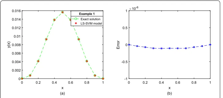
subject to two-point boundary conditionsy(0) = 0,y(0) = 0,y(1) = 0,y(1) = 0. The analytic solution isy=x3(1 –x)3.
Figure 1Two-point BVP of fourth-order nonlinear ODE (Example 1)
Table 1 Comparison between the exact solution and the LS-SVM solution (Example 1)
x Exact solution LS-SVM solution Absolute error
0.0000 0.000000000000 0.000000000217 2.1737e–10 0.0915 0.000574431275 0.000574468625 3.7350e–08 0.1518 0.002134568612 0.002134627307 5.8695e–08 0.2410 0.006120352774 0.006120441263 8.8489e–08 0.3604 0.012248409908 0.012248522843 1.1293e–07 0.5000 0.015625000000 0.015625106969 1.0697e–07 0.6395 0.012252859500 0.012252970047 1.1055e–07 0.7590 0.006120352774 0.006120442154 8.9380e–08 0.8482 0.002134568612 0.002134628711 6.0099e–08 0.9084 0.000576126428 0.000576167078 4.0650e–08 1.0000 0.000000000000 0.000000000129 1.2915e–10
the approximate solution is plotted in Fig.1(b). In spite of using fewer points, we can see that the proposed LS-SVM algorithm could have a much better performance in terms of accuracy. The mean squared error is 6.5732×10⁻¹⁵and the maximum absolute error is
approximately 1.1063×10⁻⁷.
Table1lists the results of the exact solution and the approximate solution via our pro-posed LS-SVM algorithm for 11 testing points at unequal intervals in the domain [0, 1]. The absolute errors are shown in Table1, in which we can see that the maximum absolute error is approximately 1.1293×10⁻⁷.
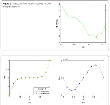
Figure2shows the logarithmic relation between the kernel bandwidth and the RMSE in Example 1. The red circle indicates the location of selected kernel bandwidth.
5.2 Example 2
Let us consider the fourth-order linear ordinary differential equation [34]:
d4y
dx4 = 120x, x∈[–1, 1], (35)
subject to two-point boundary conditionsy(–1) = 1, y(–1) = 5, y(1) = 3,y(1) = 5. The analytic solution isy=x5+ 2.
approx-Figure 2The logarithmic relation betweenσand RMSE (Example 1)
Figure 3Two-point BVP of fourth-order linear ODE (Example 2)
imate solution via our proposed LS-SVM algorithm, and Fig.3(b) depicts the error plot between the analytic solution and the approximate solution. From the obtained results, we can see that the mean squared error is 6.5835×10⁻¹²and the maximum absolute error is approximately 3.7390×10⁻⁶. The error obtained by the proposed LS-SVM algorithm
remains low for the training points.
Finally, the test results of the exact solution and the approximate solution via our pro-posed LS-SVM algorithm for 11 equidistant points in the domain [–1, 1] are listed in Ta-ble2. The absolute errors are shown in Table2, in which we can see that the maximum absolute error is approximately 3.7071×10⁻⁶. It is clear that the proposed LS-SVM
algo-rithm has a better performance in terms of accuracy.
5.3 Example 3
Consider the fourth-order linear ordinary differential equation [52]:
d4y dx4 +y(x) =
π 2
4
+ 1
cos
π 2x
, x∈[–1, 1], (36)
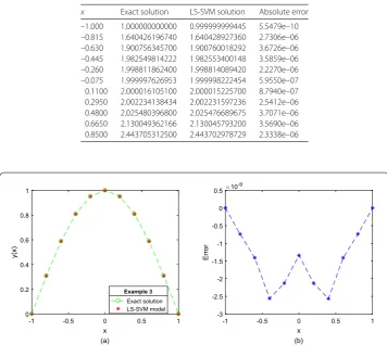
Table 2 Comparison between the exact solution and the LS-SVM solution (Example 2)
x Exact solution LS-SVM solution Absolute error
–1.000 1.000000000000 0.999999999445 5.5479e–10 –0.815 1.640426196740 1.640428927360 2.7306e–06 –0.630 1.900756345700 1.900760018292 3.6726e–06 –0.445 1.982549814222 1.982553400148 3.5859e–06 –0.260 1.998811862400 1.998814089420 2.2270e–06 –0.075 1.999997626953 1.999998222454 5.9550e–07 0.1100 2.000016105100 2.000015225700 8.7940e–07 0.2950 2.002234138434 2.002231597236 2.5412e–06 0.4800 2.025480396800 2.025476689675 3.7071e–06 0.6650 2.130049362166 2.130045793200 3.5690e–06 0.8500 2.443705312500 2.443702978729 2.3338e–06
Figure 4Two-point BVP of fourth-order linear ODE (Example 3)
The proposed LS-SVM algorithm for two-point boundary value problems of high-order linear ordinary differential equation has been trained with 11 equidistant points in the given interval [–1, 1]. Comparison between the exact solution and the approximate solu-tion via our proposed LS-SVM algorithm is depicted in Fig.4(a). Plot of the error function is cited in Fig.4(b), from which we can see that the mean squared error is 2.6426×10⁻¹⁸ and the maximum absolute error is approximately 2.5670×10⁻⁹. The accuracy of the error
obtained by the proposed LS-SVM algorithm isO(10–9). The results reveal that the
pro-posed LS-SVM algorithm has higher accuracy, although we only choose 11 equidistant points for training process.
Finally, Table3incorporates results of the exact solution and the approximate solution via our proposed LS-SVM algorithm for 11 testing points at unequal intervals in the do-main [–1, 1]. The absolute errors are shown in Table3, in which we can see that the max-imum absolute error is approximately 2.5543×10⁻⁹.
5.4 Example 4
Consider the third-order nonlinear ordinary differential equation [15]:
d3y
dx3 = –y
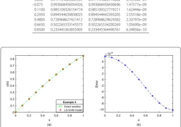
Table 3 Comparison between the exact solution and the LS-SVM solution (Example 3)
x Exact solution LS-SVM solution Absolute error
–1.000 0.000000000000000 0.000000000007191 7.19075e–12 –0.815 0.286524552727799 0.286524553452789 7.24991e–10 –0.630 0.549022817998132 0.549022819226559 1.22843e–09 –0.445 0.765483213493088 0.765483215882123 2.38904e–09 –0.260 0.917754625683981 0.917754628118062 2.43408e–09 –0.075 0.993068456954926 0.993068458430696 1.47577e–09 0.1100 0.985109326154774 0.985109327779211 1.62444e–09 0.2950 0.894544639838025 0.894544642393205 2.55518e–09 0.4800 0.728968627421412 0.728968629629382 2.20797e–09 0.6650 0.502265533143373 0.502265534200269 1.05690e–09 0.8500 0.233445363855905 0.233445364490761 6.34856e–10
Figure 5Multi-point BVP of third-order nonlinear ODE (Example 4)
subject to multi-point boundary conditionsy(0) = 1,y(12) =sin(12),y(1) =cos(1). The an-alytic solution isy=sin(x).
When 11 equidistant points in the interval [0, 1] are used for training, the results are depicted in Fig.5(a). Figure5(b) shows the errors between the exact solution and the ap-proximate solution obtained by the proposed LS-SVM algorithm. From the obtained re-sults, although training was performed just for 11 equidistant points in the domain [0, 1], the mean squared error is approximately 4.3564×10⁻⁷. The proposed LS-SVM algorithm
obtains a satisfactory result for multi-point boundary value problems of third-order non-linear ordinary differential equation.
Finally, Table4tabulates results of the exact solution and the approximate solution via our proposed LS-SVM algorithm for 11 testing points at unequal intervals in the domain [0, 1]. The absolute errors are shown in Table4, in which we can see that the mean squared error is approximately 4.9717×10⁻⁷.
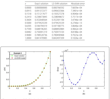
5.5 Example 5
Consider the fourth-order linear ordinary differential equation:
d4y
dx4 +
dy
dx = 4x
Table 4 Comparison between the exact solution and the LS-SVM solution (Example 4)
x Exact solution LS-SVM solution Absolute error
0.0000 0.000000000 0.000766592 7.6659e–04 0.0915 0.091372377 0.090633366 7.3901e–04 0.1518 0.151217677 0.150527278 6.9040e–04 0.2410 0.238673845 0.238098672 5.7517e–04 0.3604 0.352648564 0.352301106 3.4746e–04 0.5000 0.479425539 0.479425539 6.2766e–13 0.6395 0.596794319 0.597180775 3.8646e–04 0.7590 0.688196265 0.688892884 6.9662e–04 0.8482 0.750091219 0.750973103 8.8188e–04 0.9084 0.788520736 0.789490968 9.7023e–04 1.0000 0.841470985 0.842497209 0.1026e–04
Figure 6Multi-point BVP of third-order linear ODE (Example 5)
subject to multi-point boundary conditionsy(0) = 0,y(0.25) = 6,y(0.5) = 3,y(1) = 1. The analytic solution isy=x4.
When 21 equidistant points in the interval [0, 1] are used for training, the approximate solution obtained by the proposed LS-SVM algorithm is compared with the exact solution in Fig.6(a), and the error is plotted in Fig.6(b). From which, the mean squared error is approximately 2.2915×10⁻¹⁰. The proposed LS-SVM algorithm can obtain the desired
accuracy, although the training was performed using just a small part points in the domain [0, 1].
The test results of the exact solution and the approximate solution via our proposed LS-SVM algorithm for 20 equidistant points in the domain [0, 1] are listed in Table5, and the absolute error is also calculated in Table5. We can see that the mean squared error is approximately 2.3557×10⁻¹⁰and the maximum absolute error is approximately 2.7702×
10–5. The improved LS-SVM algorithm has a good performance for solving multi-point
boundary value problems of fourth-order linear ordinary differential equations.
6 Conclusion
Table 5 Comparison between exact solution and LS-SVM solution (Example 5)
x Exact solution LS-SVM solution x Exact solution LS-SVM solution
0.000 0.000000000000 0.000000000000 0.525 0.075969140625 0.075975418091 0.075 0.000031640625 0.000044822693 0.575 0.109312890625 0.109313011169 0.125 0.000244140625 0.000263214111 0.625 0.152587890625 0.152583122253 0.175 0.000937890625 0.000963211060 0.675 0.207594140625 0.207587242126 0.225 0.002562890625 0.002589225769 0.725 0.276281640625 0.276272773743 0.275 0.005719140625 0.005746841431 0.775 0.360750390625 0.360743522644 0.325 0.011156640625 0.011182785034 0.825 0.463250390625 0.463246345520 0.375 0.019775390625 0.019799232483 0.875 0.586181640625 0.586181640625 0.425 0.032625390625 0.032644271851 0.925 0.732094140625 0.732098579407 0.475 0.050906640625 0.050920486450 1.000 1.000000000000 1.000000000000
conditions, two fourth-order linear ordinary differential equations with two-point bound-ary conditions, a three-order nonlinear ordinbound-ary differential equation with multi-point boundary conditions, and a fourth-order linear ordinary differential equation with multi-point boundary conditions. The results obtained by the improved LS-SVM algorithms are compared with the exact solution. It has been noted that our proposed LS-SVM algo-rithms can solve two-point and multi-point boundary value problems of high-order lin-ear and nonlinlin-ear ordinary differential equations with higher accuracy in the tables and graphs. So the improved LS-SVM algorithms in the use of the two-point and multi-point boundary value problems are found to be efficient and straightforward.
Acknowledgements
The authors sincerely thank all the reviewers and the editors for their careful reading and valuable comments, which improved the quality of this paper.
Funding
This study was funded by the National Natural Science Foundation of China under Grants 61375063.
Availability of data and materials
Not applicable.
Competing interests
The authors declare that they have no competing interests.
Authors’ contributions
All authors contributed to the draft of the manuscript and all authors read and approved the final manuscript.
Publisher’s Note
Springer Nature remains neutral with regard to jurisdictional claims in published maps and institutional affiliations.
Received: 3 January 2019 Accepted: 7 May 2019
References
1. Chawla, M.M., Katti, C.P.: Finite difference methods for two-point boundary value problems involving high order differential equations. BIT Numer. Math.19, 27–33 (1979)
2. Mohyud-Din, S.T., Noor, M.A.: Homotopy perturbation method for solving fourth-order boundary value problems. Math. Probl. Eng.2007, Article ID 98602 (2007)
3. Noor, M.A., Mohyud-Din, S.T.: Homotopy perturbation method for solving sixth-order boundary value problems. Comput. Math. Appl.55, 2953–2972 (2008)
4. Ali, J., Islam, S., Islam, S., Zaman, G.: The solution of multipoint boundary value problems by the optimal homotopy asymptotic method. Comput. Math. Appl.59, 2000–2006 (2010)
5. Tatari, M., Dehghan, M.: The use of the Adomian decomposition method for solving multipoint boundary value problems. Phys. Scr.73, 672–676 (2006)
6. Wazwaz, A.M.: A new algorithm for calculating Adomian polynomials for nonlinear operators. Appl. Math. Comput. 111, 53–69 (2000)
7. Wazwaz, A.M.: The numerical solution of fifth-order boundary value problems by the decomposition method. J. Comput. Appl. Math.136, 259–270 (2001)
9. Wazwaz, A.M.: Approximate solutions to boundary value problems of higher order by the modified decomposition method. Comput. Math. Appl.40, 679–691 (2000)
10. Wazwaz, A.M.: The modified decomposition method for analytic treatment of differential equations. Appl. Math. Comput.173, 165–176 (2006)
11. Aziz, I., Siraj-ul-Islam, Nisar, M.: An efficient numerical algorithm based on Haar wavelet for solving a class of linear and nonlinear nonlocal boundary-value problems. Calcolo53, 621–633 (2016)
12. Shi, Z., Li, F.: Numerical solution of high-order differential equations by using periodized Shannon wavelets. Appl. Math. Model.38, 2235–2248 (2014)
13. Doha, E.H., Bhrawy, A.H., Hafez, R.M.: A Jacobi–Jacobi dual-Petrov–Galerkin method for third- and fifth-order differential equations. Math. Comput. Model.53, 1820–1832 (2011)
14. Doha, E.H., Abd-Elhameed, W.M., Bassuony, M.A.: New algorithms for solving high even-order differential equations using third and fourth Chebyshev–Galerkin methods. J. Comput. Phys.236, 563–579 (2013)
15. Doha, E.H., Bhrawy, A.H., Hafez, R.M.: On shifted Jacobi spectral method for high-order multi-point boundary value problems. Commun. Nonlinear Sci. Numer. Simul.17, 3802–3810 (2012)
16. Saadatmandi, A., Dehghan, M.: The use of sinc-collocation method for solving multi–point boundary value problems. Commun. Nonlinear Sci. Numer. Simul.17, 593–601 (2012)
17. Noor, M.A., Mohyud-Din, S.T.: Variational iteration technique for solving higher order boundary value problems. Appl. Math. Comput.189, 1929–1942 (2007)
18. Xu, L.: The variational iteration method for fourth order boundary value problems. Chaos Solitons Fractals39, 1386–1394 (2009)
19. Noor, M.A., Mohyud-Din, S.T.: Modified variational iteration method for solving fourth-order boundary value problems. J. Appl. Math. Comput.29, 81–94 (2009)
20. Hou, M., Han, X.: The multidimensional function approximation based on constructive wavelet RBF neural network. Appl. Soft Comput.11(2), 2173–2177 (2011)
21. Hou, M., Han, X.: Multivariate numerical approximation using constructiveL2(R) RBF neural network. Neural Comput. Appl.21(1), 25–34 (2012)
22. Hou, M., Han, X.: Constructive approximation to multivariate function by decay RBF neural network. IEEE Trans. Neural Netw.21(9), 1517–1523 (2010)
23. Yang, Y., Hou, M., Luo, J.: A novel improved extreme learning machine algorithm in solving ordinary differential equations by Legendre neural network methods. Adv. Differ. Equ.2018, 469 (2018)
24. Mall, S., Chakraverty, S.: Application of Legendre neural network for solving ordinary differential equations. Appl. Soft Comput.43, 347–356 (2016)
25. Rudd, K., Ferrari, S.: A constrained integration (CINT) approach to solving partial differential equations using artificial neural networks. Neurocomputing155, 277–285 (2015)
26. Sun, H., Hou, M., Yang, Y., Zhang, T., Weng, F., Han, F.: Solving partial differential equation based on Bernstein neural network and extreme learning machine algorithm. Neural Process. Lett. (2018).
https://doi.org/10.1007/s11063-018-9911-8
27. Yang, Y., Hou, M., Sun, H., Zhang, T., Weng, F., Luo, J.: Neural network algorithm based on Legendre improved extreme learning machine for solving elliptic partial differential equations. Soft Comput. (2019).
https://doi.org/10.1007/s00500-019-03944-1
28. Zuniga-Aguilar, C.J., Romero-Ugalde, H.M., Gomez-Aguilar, J.F., et al.: Solving fractional differential equations of variable-order involving operators with Mittag–Leffler kernel using artificial neural networks. Chaos Solitons Fractals 103, 382–403 (2017)
29. Rostami, F., Jafarian, A.: A new artificial neural network structure for solving high-order linear fractional differential equations. Int. J. Comput. Math.95(3), 528–539 (2018)
30. Pakdaman, M., Ahmadian, A., Effati, S., et al.: Solving differential equations of fractional order using an optimization technique based on training artificial neural network. Appl. Math. Comput.293, 81–95 (2017)
31. Chaharborj, S.S., Chaharborj, S.S., Mahmoudi, Y.: Study of fractional order integro–differential equations by using Chebyshev neural network. J. Math. Stat.13(1), 1–13 (2017)
32. Zhou, T., Liu, X., Hou, M., Liu, C.: Numerical solution for ruin probability of continuous time model based on neural network algorithm. Neurocomputing331, 67–76 (2019)
33. Chakraverty, S., Mall, S.: Regression based weight generation algorithm in neural network for solution of initial and boundary value problems. Neural Comput. Appl.25, 585–594 (2014)
34. Malek, A., Beidokhti, R.S.: Numerical solution for high order differential equations using a hybrid neural network–optimization method. Appl. Math. Comput.183, 260–271 (2006)
35. Mai-Duy, N.: Solving high order ordinary differential equations with radial basis function networks. Int. J. Numer. Methods Eng.62(6), 824–852 (2005)
36. Vapnik, V.N.: The Nature of Statistical Learning Theory, 1st edn. Springer, New York (1995)
37. Suykens, J.A.K., Vandewalle, J.: Least squares support vector machine classifiers. Neural Process. Lett.9(3), 293–300 (1999)
38. Yang, Y., Tan, M., Dai, Y.: An improved CS-LSSVM algorithm-based fault pattern recognition of ship power equipments. PLoS ONE12, 1–10 (2017)
39. Liu, X., Bo, L., Luo, H.: Bearing faults diagnostics based on hybrid LS-SVM and EMD method. Measurement59, 145–166 (2015)
40. Yu, L., Chen, H., Wang, S., Lai, K.K.: Evolving least squares support vector machines for stock market trend mining. IEEE Trans. Evol. Comput.13, 87–102 (2009)
41. Junga, H.C., Kimb, J.S., Heo, H.: Prediction of building energy consumption using an improved real coded genetic algorithm based least squares support vector machine approach. Energy Build.90, 76–84 (2015)
42. Mehrkanoon, S., Falck, T., Suykens, J.A.K.: Approximate solutions to ordinary differential equations using least squares support vector machines. IEEE Trans. Neural Netw. Learn. Syst.23(9), 1356–1367 (2012)
44. Mehrkanoon, S., Suykens, J.A.K.: LS-SVM approximate solution to linear time varying descriptor systems. Automatica 48, 2502–2511 (2012)
45. Zhang, G., Wang, S., Wang, Y.: LS-SVM approximate solution for affine nonlinear systems with partially unknown functions. J. Ind. Manag. Optim.10, 621–636 (2014)
46. Wang, Q., Wang, K., Chen, S.: Least squares approximation method for the solution of Volterra–Fredholm integral equations. J. Comput. Appl. Math.272, 141–147 (2014)
47. Mehrkanoon, S., Suykens, J.A.K.: Deep hybrid neural–kernel networks using random Fourier features. Neurocomputing298, 46–54 (2018)
48. Suykens, J.A.K., Gestel, T.V., Brabanter, J.D., Moor, B.D., Vandewalle, J.: Least Squares Support Vector Machines. World Scientific, Singapore (2002)
49. Kincaid, D.R., Cheney, E.W.: Numerical Analysis: Mathematics of Scientific Computing, 3rd edn. Brooks/Cole, Pacific Grove (2002)
50. Arfken, G.B., Weber, H.J.: Mathematical Methods for Physicists, 4nd edn. Academic Press, New York (1995) 973. 51. Gamel, M.E., Behiry, S.H., Hashish, H.: Numerical method for solution of special nonlinear fourth-order boundary value
problems. Appl. Math. Comput.145, 717–734 (2003)