Optimal temporal planning using the plangraph framework

Dinh, Tien Ba

Optimal temporal planning using the plangraph framework Original Citation

Dinh, Tien Ba (2007) Optimal temporal planning using the plangraph framework. Doctoral thesis,  University of Huddersfield. 

This version is available at http://eprints.hud.ac.uk/id/eprint/250/

The University Repository is a digital collection of the research output of the University, available on Open Access. Copyright and Moral Rights for the items on this site are retained by the individual author and/or other copyright owners. Users may access full items free of charge; copies of full text items generally can be reproduced, displayed or performed and given to third parties in any format or medium for personal research or study, educational or not­for­profit purposes without prior permission or charge, provided:

• The authors, title and full bibliographic details is credited in any copy; • A hyperlink and/or URL is included for the original metadata page; and • The content is not changed in any way.

For more information, including our policy and submission procedure, please contact the Repository Team at: [email protected].

Tien Ba Dinh

A thesis submitted to the University of Huddersfield

in partial fulfilment of the requirements for

the degree of Doctor of Philosophy

The University of Huddersfield

The past few years have seen a rapid development in AI Planning and Scheduling. Many

algorithms and techniques have been studied and improved to deal with more complex and

difficult planning domains.

One such innovation wasGraphplan, first developed by Blum and Furst in 1995 and soon became one of the best approaches for optimal classical planning systems. Planning

sys-tems that use Graphplan’s plangraph framework can find optimal plans for temporal

plan-ning problems, in which actions have durations. However, these systems have had strict

assumptions on the preconditions and effects of actions, for instance, effects happen only

at the end of the execution. In addition, the algorithm used in the solution extraction phase

of these plangraph-based systems does not take full advantage of the information provided

by the expansion phase to prune irrelevant search branches early.

With the ambition to make temporal planning problems more realistic, the thesis proposes

an extension to the Planning Domain Definition Language (PDDL) 2.1 level 3, to allow

actions to have intermediate effects. Our optimal temporal planning system, CPPlanner,

is introduced as the first Graphplan-based optimal planner to handle the richer temporal

domains (i.e. actions can have intermediate effects). Futhermore, the planner applies

“crit-ical paths” as a backbone for the search in the solution extraction phase, so that irrelevant

search branches are pruned early. This improves the performance even in more restricted

temporal planning domains.

In our experimental evaluation, CPPlanner outperforms two leading plangraph-based

opti-mal temporal planning systems, TGP and TPSYS, in almost all test cases. The

state-of-the-art optimal planner CPT and latest temporal planning domains in the international planning

First of all, I would like to thank my supervisors Prof. Barbara Smith and Prof. Lee

McCluskey for all their help, advice, encouragement, and friendship throughout. With

their inspiration, and help, the PhD research became easier and more attractive to me.

I would like to thank Dr. Ian Miguel for his help on ILOG Solver and AI Planning, Dr.

Stephen Cresswell for his help in compiling TGP, and fixing the parser for TPSYS, and Dr.

Diane Kitchin for her advice and enthusiasm.

I would like to thank all members of the ARTFORM research group, who have also helped

me and inspired me.

Many thanks to the staff at the University of Huddersfield, especially the technical and the

administrative staff, for their promptly support on any problems that I have encountered.

I would like to express my gratitude to my best friend, Dr. Damian Jenkinson, for his

kindness and support, especially his offer on accommodation during the writing-up stage.

I am grateful to CoThu, ChuMao, beNa, Vi, Thuy and anhTuan, who are like my family

members in England, for their help, consideration, and encouragement throughout. I will

never forget the beautiful time in Stockport.

I would like to thank Prof. Duong Anh Duc, all of my friends, and staff members at the

Faculty of Information Technology at the University of Natural Sciences, Ho Chi Minh

City, Vietnam for their support and encouragement.

I wish to show my appreciation to my girlfriend Le Hong Van for her love, support and

encouragement throughout.

Finally, and most importantly, my grandmother, parents, brother, and sisters have been

both supportive and encouraging throughout the completion of this thesis, for which I am

List of Figures vii

List of Tables ix

Chapter 1: Introduction 1

1.1 Thesis structure . . . 3

1.2 Contributions . . . 4

Chapter 2: Introduction to Artificial Intelligence Planning 6 2.1 Introduction . . . 6

2.2 Classical planning . . . 9

2.2.1 Introduction . . . 9

2.2.2 Classical planning representations . . . 10

2.2.2.1 Classical representation . . . 10

2.2.3 Introduction to planning approaches . . . 11

2.2.4 State-space planning . . . 12

2.2.4.1 Introduction . . . 12

2.2.4.2 Progressive search . . . 12

2.2.4.3 Regressive search . . . 13

2.2.4.4 STRIPS algorithm . . . 14

2.2.5 Plan-space planning . . . 15

2.2.5.1 Introduction . . . 15

2.2.5.2 Search space . . . 16

2.2.6.2 Description . . . 18

2.2.6.3 Mutual exclusion . . . 18

2.2.6.4 Graphplan planner . . . 20

2.2.7 Constraint Programming in planning . . . 21

2.2.7.1 Introduction . . . 21

2.2.7.2 Constraint Satisfaction Problem . . . 21

2.3 Planning with time and resources . . . 22

2.3.1 Planning with time . . . 22

2.3.1.1 Introduction . . . 22

2.3.1.2 Temporal representation . . . 23

2.3.1.3 Approaches in temporal planning systems . . . 24

2.3.2 Planning with resources . . . 25

2.3.2.1 Introduction . . . 25

2.3.2.2 Approaches . . . 26

2.4 Planning Domain Definition Language (PDDL) . . . 27

2.4.1 Introduction . . . 27

2.4.2 PDDL . . . 28

2.4.3 PDDL 2.1 . . . 34

2.4.4 PDDL 2.2 . . . 40

2.4.5 PDDL 3 . . . 41

2.5 An extension of PDDL2.1 level 3 to handle intermediate effects . . . 43

2.5.1 Introduction . . . 43

2.5.2 Syntax and semantics . . . 44

2.6 Summary . . . 47

3.2 Temporal Planning Systems . . . 49

3.2.1 Graphplan-based temporal planners . . . 49

3.2.1.1 Introduction . . . 49

3.2.1.2 Temporal Graphplan (TGP) . . . 50

3.2.1.3 Temporal Planning System (TPSYS) . . . 52

3.2.1.4 Linear-Programming GraphPlan (LPGP) . . . 54

3.2.2 Partial Order Planners . . . 55

3.2.2.1 Introduction . . . 55

3.2.2.2 parcPLAN . . . 56

3.2.2.3 IxTeT . . . 57

3.2.2.4 Zeno . . . 59

3.2.2.5 Constraint Programming Temporal planner (CPT) . . . . 61

3.2.3 Heuristic Planners . . . 63

3.2.3.1 Introduction . . . 63

3.2.3.2 Sapa . . . 63

3.2.3.3 TP4 . . . 64

3.3 Summary . . . 66

Chapter 4: CPPlanner - An Optimal Temporal Planning System using Crit-ical Paths 68 4.1 Introduction . . . 68

4.1.1 Towards the new extension of the plangraph framework . . . 69

4.2 Action representation . . . 69

4.3 The planning graph . . . 71

4.4 Graph Expansion . . . 73

4.4.1 The concept . . . 73

4.6 Solution Extraction . . . 84

4.6.1 The concept . . . 84

4.6.2 Critical Path extraction . . . 87

4.6.3 The algorithm description . . . 89

4.7 Summary . . . 92

Chapter 5: Improvements 94 5.1 Introduction . . . 94

5.2 Avoid redundant solution extraction calls . . . 94

5.3 Conflict Directed Backjumping . . . 95

5.3.1 Motivation . . . 95

5.3.2 Improving the search with Conflict-Directed Backjumping . . . 97

5.4 Summary . . . 97

Chapter 6: Experiments and empirical analysis 98 6.1 Introduction . . . 98

6.2 Temporal planning domains used in the experiments . . . 99

6.2.1 Temporal domainlogisticsextracted from the TGP package . . . . 100

6.2.2 Temporal domains extracted from IPC2002 . . . 101

6.2.2.1 Depots . . . 101

6.2.2.2 DriverLog . . . 102

6.2.2.3 Satellite . . . 104

6.2.2.4 Rovers . . . 104

6.2.2.5 ZenoTravel . . . 106

6.2.3 Airport- a temporal domains extracted from the IPC2004 . . . 107

6.2.4 Storage- A temporal planning domain extracted from IPC2006 . . 108

6.3.2 Temporal planning domains from IPC2002 . . . 115

6.3.3 TheAirporttemporal domain extracted from IPC2004 . . . 117

6.3.4 TheStoragetemporal domain extracted from the latest IPC2006 . . 118

6.3.5 Spacecraft - A temporal domain with intermediate effects . . . 120

6.4 Summary of the empirical study and discussion . . . 121

Chapter 7: Conclusion and future work 123 7.1 Introduction . . . 123

7.2 Summary of contributions . . . 123

7.2.1 CPPlanner algorithm . . . 123

7.2.1.1 “Critical paths” . . . 123

7.2.1.2 Extension to the algorithm to handle intermediate effects 124 7.2.2 Extension to PDDL2.1 level 3 . . . 124

7.2.3 CPPlanner - a new optimal planning system for temporal planning domains . . . 125

7.3 Further developments . . . 126

7.3.1 Memoisation . . . 126

7.3.2 Heuristic search . . . 126

7.3.3 Using current Constraint Programming Solvers . . . 127

7.4 ...and finally . . . 128

Bibliography 129 Appendix A: Comparisons a same planner on different operating systems 142 Appendix B: Planning domains and problems used in the experiment 145 B.1 Logistics domain from the TGP package . . . 145

B.2.1 Depot . . . 147

B.2.2 DriverLog . . . 149

B.2.3 Satellite . . . 153

B.2.4 Rovers . . . 155

B.2.5 ZenoTravel . . . 161

B.3 Airport domain extracted from IPC2004 . . . 163

B.4 Domain storage extracted from IPC2006 . . . 174

B.5 Domainspacecraftwith intermediate effects . . . 177

2.1 The abstract view of components in a planning system . . . 7

2.2 Pseudo-code forProgressiveSearch (O, s0, g)extracted from [42]. . . 13

2.3 Pseudo-code forRegressiveSearch (O, s0, g)extracted from [42]. 14 2.4 Pseudo-code forSTRIPS (O, s, g)extracted from [42]. . . 15

2.5 Pseudo-code for plan-space planningPSP (π)extracted from [42]. . . 17

2.6 The overview of a planning graph . . . 19

2.7 A part of gripper domain extracted from planning competition 1998 . . . . 30

2.8 Jug-pouring domain description, extracted from the AI Magazine article [73] 31 2.9 Vehicle domain description, extracted from Fox and Long’s paper [37] . . . 33

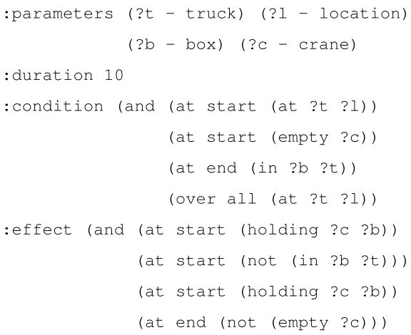
2.10 Jug-pouring domain description, extracted from PDDL 2.1 document [37] . 35 2.11 Offloading a box from a truck . . . 36

2.12 Flying from one place to another . . . 37

2.13 A part of bath-filling domain, extracted from PDDL+ [35] . . . 39

2.14 An example of a derived predicate . . . 40

2.15 Turning the spacecraft from the current target to a new target . . . 46

3.1 The causation diagram of the TGP graph expansion phase. Dark lines mean the effects happen later in time (i.e. after action execution). The figure is extracted from TGP paper [88] . . . 51

3.2 The overview of the planning graph of LPGP with duration attached to proposition level and actions are divided into smaller actions. Figure is extracted from the LPGP paper [67] . . . 54

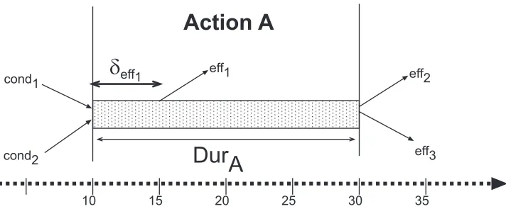
4.1 Action representation . . . 71

4.2 The multiple-level planning graph of the plangraph approach . . . 72

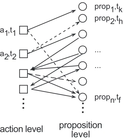
4.3 The Bi-level planning graph . . . 73

4.4 The model of a plangraph-based planning system . . . 74

4.5 The Graph Expansion Diagram . . . 76

4.6 Pseudo-code forGraphExpansion(). . . 79

4.7 Pseudo-code forApplyingPossibleActions(). . . 80

4.8 Action turning of the spacecraft domain. The vibration effects prevent actioncamera chance1but notcamera chance2. . . 82

4.9 The diagram of the solution extraction . . . 85

4.10 Pseudo-code to get a decisive proposition for an action. . . 87

4.11 Pseudo-code to get all possible paths for a certain subgoal. . . 88

4.12 Pseudo-code forCriticalPath candidates extraction (). . . 88

4.13 The planning graph after the expansion phase. Note that for simplicity the full level graph is used for the illustration purpose . . . 90

4.14 Pseudo-code forSolutionExtraction (). . . 91

5.1 An example to illustrate the inefficiency in the backtracking of the solution extraction phase . . . 95

6.1 The numbers of objects in each problem of theLogisticsdomain extracted

from the TGP package. . . 101

6.2 The numbers of objects in each problem of theDriverLogdomain extracted

from IPC2002. . . 103

6.3 The numbers of objects in each problem of theSatellitedomain extracted

from IPC2002. . . 105

6.4 The numbers of objects in each problem of the Rover domain extracted

from IPC2002. . . 106

6.5 The numbers of objects in each problem of the ZenoTravel domain

ex-tracted from IPC2002. . . 107

6.6 The numbers of objects in each problem of theAirport domain extracted

from IPC2004. . . 108

6.7 The numbers of objects in each problem of the Storagedomain extracted

from IPC2006. . . 110

6.8 The numbers of objects in each problem of theSpacecraftdomain . . . 112

6.9 The comparison of different planning systems on the Logistics domain.

Time is in seconds to find an optimal solution. . . 114

6.10 Comparison to TPSYS on IPC2002 temporal planning domains. Time is in

seconds to find an optimal solution. . . 116

6.11 Comparison to CPT on theAirportplanning domain in the IPC2004. Time

is in seconds to find an optimal solution. . . 118

6.12 Comparison to CPT2 on theStorageplanning domain in the latest IPC2006.

Time is in seconds to find an optimal solution. . . 119

A.1 Comparison of CPT on Windows XP and Linux MEMPIS on domain

Air-portextracted from IPC2004. Time is in seconds to find an optimal solution. 142

A.2 Comparison of CPT on Windows XP and Linux MEMPIS on domain

Satel-liteextracted from IPC2004. Time is in seconds to find an optimal solution. 143

INTRODUCTION

It is hard to establish when Artificial Intelligence Planning (AI Planning) was first

in-troduced. It is known that AI Planning was already considered to be a subfield of Artificial

Intelligence in the late 1960s. AI Planning applications can now be found in different fields,

such as autonomous manufacturing, space exploration, and the game industry.

In our daily lives, planning problems are everywhere, e.g. going to school, going

shop-ping etc. Any of us is able to find plans in these situations. However, we have little

knowledge on how our brains work to find the solutions. The mechanism to find a good

plan for a planning problem is still a challenge to scientists nowadays.

One of the very first planning problems considered in AI was the monkey-banana

prob-lem which was proposed by John McCarthy in 1963 [70]. The initial state tells the position

of the monkey, the banana, and the chair. With actions such as walk, move the chair to

underneath the hanging banana, climb etc., the solution is a sequence of actions for the

monkey to get the banana (i.e. the goal state). In this example, John McCarthy introduced

the idea of modelling planning domains into situation calculus by using axioms.

Planning systems and definitions were gradually proposed and developed. However,

each research group developed their own planning system with their own specification

lan-guage for describing a planning domain. This was the situation until 1998, in order to

pre-pare for the first international planning competition, Drew McDermott and other members

of the committee proposed the first Planning Domain Definition Language (PDDL) [72]

to the planning community. Since then, planning systems are compared more easily using

PDDL. PDDL has been developed and extended further to model real-world domains, and

In 1995, Blum and Furst first introduced Graphplan [13] to the planning community.

The algorithm’s innovation is in forming the union of all the reachable states of a current

state together to reduce space complexity, and in finding a solution in a later stage by

backtracking search. This introduction was a big step forward in dealing with planning

problems. Years later, scientists are still working within the plangraph framework to handle

more complex problems, e.g. in temporal planning or planning with resources. Some have

extended the plangraph framework to find an optimal solution for temporal planning, while

others have used the relaxed planning graph as a part of the heuristic function for

state-space search.

However, planning is still a long way from being able to solve realistic problems

ef-ficiently. Planning problems are generally NP-complete [30], even the simple famous

BlocksWorld problems.

At the start of the research described in this thesis, TGP [88] and TPSYS [38] were

the two well-known plangraph-based optimal planning systems for temporal planning

do-mains. These planning system use the plangraph framework to find a plan with minimal

makespan. However, there are several limitations of these two systems, such as a strict

as-sumption on conditions and effects while executing actions. Effects of actions are allowed

only at the end of the action in TGP and only at the beginning or at the end in TPSYS.

Also, the approaches used in the solution extraction phase does not take advantage of all

the information available after the graph expansion phase. This motivated us to develop

CPPlanner. CPPlanner extends PDDL2.1 to allow actions with intermediate effects and

handles them using the plangraph framework. It also uses “critical paths” provided by the

expansion phase to add some actions and propositions to the final plan before the actual

backtracking search takes place. Other improvements are introduced to CPPlanner to speed

1.1 Thesis structure

The thesis is constructed as follows:

• Chapter 2: Introduction to Artificial Intelligence Planning. This chapter introduces

AI Planning. It begins with the definition of what is a planning problem, and a

so-lution to a planning problem. Different types of planning and approaches are

intro-duced. Then, the Planning Domain Definition Language (PDDL) with its extensions

is described briefly. The syntax and semantics of actions with intermediate effects

are proposed in this chapter. This extension allows actions of the current PDDL 2.1

level 3 to have intermediate effects.

• Chapter 3: Temporal Planning Systems. This chapter gives an overview of

well-known temporal planning systems. Each temporal planner is introduced briefly and

its capabilities discussed. The chapter focuses on TGP [88] and TPSYS [38], which

are the two main plangraph-based optimal temporal planning systems. These two

planners will be considered and compared directly to our system in the experimental

study.

• Chapter 4: CPPlanner - An Optimal Temporal Planning System using Critical Paths.

The chapter describes the CPPlanner framework. It begins with the plangraph

frame-work and extends it to deal with temporal domains. Extensions to handle

interme-diate effects are also illustrated. The details of the algorithms for both the graph

expansion phase and solution extraction are described fully. The use of “critical

paths”, which is one of the main contributions, is analysed and shown in detail. A

simple example is also included to illustrate the algorithm.

• Chapter 5: Improvements. This chapter contains the improvements to CPPlanner.

It introduces the timebound in selecting next actions for the search in the solution

to CPPlanner to help the planner jump right back to the origin of the conflict. These

improvements are developed and described in detail.

• Chapter 6: Experiments and empirical analysis. This chapter illustrates the

per-formance and comparison of CPPlanner to TGP and TPSYS on different temporal

domains. The domains are mainly from the planning competitions and the TGP

package. In addition, CPPlanner is compared to the state-of-the-art optimal

tem-poral planning system, CPT in latest temtem-poral planning domains in the last two

in-ternational planning competitions, IPC2004 and IPC2006. This chapter also shows

the comparison of CPPlanner with the earlier version of CPPlanner, called

CPPlan-ner Basic which does not include “critical paths” in the solution extraction phase and

the improvements of chapter 5.

• Chapter 7: Conclusion and future work. This chapter contains the summary of

con-tributions of this thesis. It also incudes the future directions for CPPlanner.

• Appendix A: Comparisons a same planner on different operating systems. The

chap-ter shows the empirical study of the performance of a planning system on different

platforms. It illustrates there is not much difference in running time if planning

sys-tems are compared under the same hardware settings but on different platforms.

• Appendix B. The chapter contains the details of test suites which were used in the

empirical study.

1.2 Contributions

This section introduces and outlines the main contributions of this thesis:

• Introduction of intermediate effects to PDDL2.1 level 3. Because of the complexity

planning, the extension in syntax and semantics of PDDL2.1 is introduced. This

introduction helps to move planning problems towards real-world problems.

• “Critical paths”. This new idea improves the performance of plangraph-based

tem-poral planning systems. The introduction of “critical paths” helps the solution

extrac-tion phase add acextrac-tions and proposiextrac-tions before the actual search takes place. Note

that with actions and propositions being added to the plan early, the search for

so-lutions will be improved even when actions do not have intermediate effects.

Time-bounds and conflict directed-backjumping are also introduced to the backtracking

search of the solution extraction phase to reduce the search space.

• Development of CPPlanner. CPPlanner is developed with the ability to handle

tem-poral planning domains with intermediate effects. The new improvements of the

solution extraction phase are included and tested. The planner shows the efficiency

of the development via experimental results.

• Empirical analysis of CPPlanner and the introduction of a planning domains with

intermediate effects. It contributes to the planning community the comparison of

CPPlanner and other optimal temporal planning systems, TGP and TPSYS, on many

temporal planning problems. The comparison to CPT is also included. Especially, a

new temporal planning domain with actions and intermediate effects are introduced.

INTRODUCTION TO ARTIFICIAL INTELLIGENCE PLANNING

2.1 Introduction

Artificial Intelligence planning (AI planning) has been a sub-field of Artificial Intelligence

since the 1960s [79, 70, 71, 44]. It is a well-known area in Artificial Intelligence that studies

to build algorithms and techniques for planning. AI Planning is applied in many areas in

the real world such as automated data-processing [43, 17], autonomous manufacturing [75]

and [45], space exploration [74, 18, 86, 57], robotics [11, 10, 12, 9], game industry [93],

and large-scale logistics problems [104]. Scientists have studied and developed efficient

algorithms and models to deal with real world problems due to their size and complexity.

An overview of progresses and algorithms in AI Planning can be found in [101, 87, 66].

This chapter will describe briefly the definition of planning problems, types of planning,

approaches and techniques, and the description language used in the International Planning

Competitions: PDDL.

Firstly, it is necessary to define what is a planning problem. Different researchers have

different definitions of planning problems. However, below is the common definition of

what is a planning problem.

Definition 2.1 A planning problem is described as an initial state containing propositions,

a goal state (i.e. a set of propositions called subgoals) to be achieved, and a collection of

actions, in which each has a set of preconditions (which need to be true for the action to

be executed) and a set of effects (which will be true when the action is applied).

will transform the initial state to a state that satisfies all the propositions/subgoals of the

goal state.

In everyday usage, planning is the process of finding a plan for a given initial state and

goal state before actually executing any of them. For example, when we are cooking, we

have a plan which shows a sequence of actions that we will follow. These actions have to

be followed in a predefined order.

initial

state

actions

execution

the world

goal

state

planning

Domain

Model

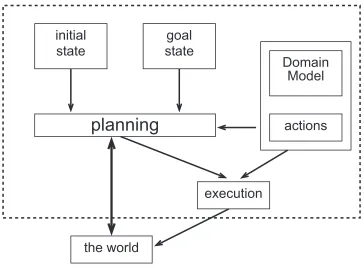
Figure 2.1: The abstract view of components in a planning system

Figure 2.1 shows the general view of components of a planning system. Given a initial

state, a goal state, and a list of available actions, the planning system looks for a sequence

of actions to achieve the goal state. When the plan is executed, the actions are applied to

change from one state to another in the world to achieve the pre-defined goal state. The

initial state, the goal state and actions are defined depending on the type of planning and

With the hope of encouraging researchers to share their planning problems and

algo-rithms, as well as to allow comparisons on performance of different planning systems, the

Planning Domain Description Language (PDDL) was first proposed in 1998 by a

commit-tee led by McDewmott [72], and then extended by Fox and Long in 2002 [34], EdelKamp

and Hoffmann in 2004 [27], and Gerevini and Long in 2006 [40]. The language has been

used as a standard for modelling planning problems. The detail of the language is discussed

later in this chapter.

AI Planning is categorized into different types, such as classical planning, planning

with time and resources, planning under uncertainty, according to the expressivity of the

representation of the planning problem (or the planning language required to describe the

planning problem). The more expressive the planning language is, the bigger the search

space to find a plan becomes. In the scope of this thesis, classical planning and its

ap-proaches are introduced and described briefly. The main focus is on temporal planning (i.e.

planning with time).

However, there are other ways to classify a planning system. It can be classified as a

domain-independent planner, or adomain-dependent planner, in which some hand-coded

knowledge is provided for the domain.

Besides, planning systems might be classified according to the algorithms and

tech-niques used, such as Graphplan-based planners (e.g. IPP [60], STAN [33], TGP [89]), SAT

planners [56, 54], and HTN planners [103, 19, 76] etc.

The next sections introduce classical planning, and planning with time and resources.

In each section, the representation and planning approaches, including algorithms and

2.2 Classical planning

2.2.1 Introduction

Early research in AI Planning was related to automated theorem proving [44]. In these

systems, the initial state, goal state and actions are described in terms of axioms. Resolution

theorem proving was used to produce a proof that a plan exists, and the actual plan found

by applying answer extraction to the proof. However, those systems faced difficulties when

it was required to specify axiomatically not only the changes that an action makes to a state

but also the elements left unchanged. This encouraged the development of the classical

formulation which introduced a simple solution to those types of problems.

Classical planning is a type of planning for restricted state-transition systems. These

restricted systems have the following assumptions:

• The system has a finite set of states.

• The system is fully observable.

• The system is deterministic, i.e. a possible application of an action to a state only

brings it to a single other state.

• The state remains unchanged until another application of an action.

• Actions have no duration.

• Goals are restricted and explicit. It means there are no constraints or conditions on

the goal state.

• The solution is a sequence of linearly ordered finite actions.

2.2.2 Classical planning representations

In AI Planning, it is essential to have a description of the planning problem for planners.

There are different types of representations [42] for classical planning: set-theoretic

rep-resentation,classical representation, andstate-variable representation. These

representa-tions have equivalent expressivity. It means that a planning problem can be represented

equally well in any of those representations. In AI Planning, the classical representation

is the most popular and often used by the community. The section below describes the

classical representation.

2.2.2.1 Classical representation

In classical representation, states are represented as a set of logical atoms. Actions are

represented asoperatorswhich change the truth values of atoms.

Firstly, the first-order language L has finite predicate symbols and constant symbols,

but no function symbols. A state is a set of atoms of L. Because L is finite and has no

function symbol, the set of all possible statesSis finite.

Definition 2.3 An operator is a tripleo= (name(o), precond(o), effect(o)), in which:

• name(o) is the name of the operator. It is an expression in the form of n(x1, ...,xk)

where n is the operator symbol, and is unique; and every xi is a variable symbol

which can appear anywhere ino.

• precond(o) and effect(o) are preconditions and effects of the operator. These

precon-ditions and effects are sets of literals (i.e. atoms and negations of atoms).

• The application of an instance of the operator to a state is described as follows:γ(s,

a) = (s\effect−_{(a))∪effect}+_(a).

Definition 2.4 LetLbe a first-order language, aclassical planning domainis a restricted

• S⊆2{allgroundatomsofL}

• A ={all ground instances of operators inO}

• γ(s, a) = (s\effect−_{(a))∪effect}+_{(a), if ais applicable to the states. The new state}

constructed is inSas well.

Definition 2.5 Aclassical planning problemis tripleP= (Σ,s0,g), in which:

• s0is the initial state.

• gis the goal state - a set of literals which need to be achieved.

2.2.3 Introduction to planning approaches

There are many different algorithms and techniques to deal with a wide variety of planning

problems [87]. Some planning systems solve planning problems by searching through a

graph representing the state space [77, 50, 6]. Each node in this space presents a state of

the world. Arcs are state transitions or actions. Therefore, a plan is a path starting from

the initial state, going through intermediate states, and ending at a goal state by applying a

sequence of actions. This is calledstate space planning.

Other planning systems solve planning problems by searching through a space of plans

[82, 8]. This approach is calledplan space planning. Each node in this space is a partially

specified plan. Arcs are plan refinement operations to achieve an open goal or to remove

a possible inconsistency. In this approach, the planning system starts from an initial node

which is an empty plan. The planner, then, is aiming at the final node containing a plan,

which achieves the goal.

The planning graph approach is a synthesis of state space planning and plan space

planning. It introduces a compact and powerful search space, which is called aplanning

graph. Starting from the initial state, also called the first level, the approach builds a next

same level, if two or more states have parts in common, those parts are stored only once.

Hence, the size of the graph is much smaller than the graph in the state space planning.

In addition, there are other approaches which apply Constraint Programming (CP),

Satisfiability (SAT) techniques, or heuristics.

Those approaches can be applied to both classical planning and planning with time

and resources. In the next sections, the classical representation is used in describing the

approaches for classical planning. For planning with time and resources, the planning

systems can use the same approaches but with extensions.

2.2.4 State-space planning

2.2.4.1 Introduction

As described earlier, in state-space planning, each node represents a state of the world. Arcs

are state transitions. The solution plan is a path in the search space. In classical planning,

classical state-space search algorithms are easy to understand. There are two approaches:

progressive andregressive search: starting from the state representing the initial state or

goal state respectively, the planning system searches through the state space to find the

solution path leading to the goal state or initial state respectively. These two approaches

are discussed in more detail in the following sections.

2.2.4.2 Progressive search

Progressive search, also known asforwardsearch, is one of the simplest search algorithms

in AI Planning. Starting from the initial state, the planner searches the state space to find

a solution path leading to the goal state. Figure 2.2 is a general pseudo-code example of a

progressive search algorithm in AI Planning:

In figure 2.2, the algorithm is a depth-first backtracking search. The algorithm might

end up in an infinite search branch if there is a state si with i < kin the sequence s0, s1,

01. ProcedureProgressiveSearch(O,s₀,g) 02. s←s0

03. π← {}//an empty plan

04. Loop

05. ifgis a subset of s then returnπas the solution plan and terminate 06. // store the list of all possible actions

07. possActions←a|a∈O and precond(a) is satisfied ins

08. IfpossActions=∅thenreturn failure and backtrack 09. // Try each action in the possible list

10. Foreach aiinpossActionsdo

11. s←γ (s, ai)

12. π←πLai

13. run theloopto continue

14. od{end for}

15. End{loop}

Figure 2.2: Pseudo-code forProgressiveSearch (O, s0, g)extracted from [42].

return to this state. In order for the algorithm to be complete, these infinite search branches

must be pruned (i.e. the algorithm must check and return failure at any time it finds a state

which is the same as a state earlier in the listπ).

2.2.4.3 Regressive search

Regressive search, also known asbackwardsearch, is another approach in state-space

plan-ning. The solution plan is extracted from the state space by starting the search from the

goal state, traversing through other states backwards, and ending at the initial state. The

figure 2.3 shows the pseudo-code of the regressive search.

Like the progressive search, the regressive search also keeps a record of the list of state

01. ProcedureRegressiveSearch(O,s₀,g) 02. s←g

03. π← {}//an empty plan

04. Loop

05. ifs₀is a subset of s then returnπas the solution plan and terminate 06. // store the list of all possible actions

07. possActions←a|a∈O and effect(a)∩s6=∅

08. IfpossActions=∅thenreturn failure and backtrack 09. // Try each action in the possible list

10. Foreach aiinpossActionsdo

11. s←γ−1_{(s, a}

i)

12. π←ai

L π

13. run theloopto continue

14. od{end for}

15. End{loop}

Figure 2.3: Pseudo-code forRegressiveSearch (O, s0, g)extracted from [42].

failure whenever it finds a state sj, in which j>k and sj ⊆sk.

2.2.4.4 STRIPS algorithm

In the previous two sections, the progressive and regressive search are introduced.

How-ever, the size of the search space is very big. The STRIPS algorithm [31], which was

developed by Fikes and Nilsson in 1971 at Stanford university, is one of the first attempts

to reduce the search space. The algorithm is very similar to regressive search, but is

differ-ent in the following respects:

• In each recursive call to the STRIPS algorithm, only actions which have a part of their

effects in common with the preconditions of the last chosen action are considered.

01. ProcedureSTRIPS(O,s,g) 02. π← {}// an empty plan

03. Loop

04. ifssatisfies g then returnπ

05. A← {a|ais a ground instance of an operator in O, 06. and a is relevant forg}

07. if A =∅then return failure.

08. choose any actiona∈A nondeterministically. 09. π’←STRIPS(O,s, precond(a))

10. ifπ’ = failure then failure

11. s←γ−1_(s,π’) 12. s←γ−1_(s,a) 13. π←π.π’.a

15. End{loop}

Figure 2.4: Pseudo-code forSTRIPS (O, s, g)extracted from [42].

• If at the current state, an action has all of its preconditions satisfied, STRIPS will

execute the action and not backtrack over this commitment.

2.2.5 Plan-space planning

2.2.5.1 Introduction

This section introduces plan-space planning. In state-space planning, nodes represent states

of the search space, arcs are transitions or actions between states, and a solution plan is a

path of states from the initial state to the goal state. However, in plan-space planning, as

described earlier, nodes arepartially specified plans. Arcs areplan refinement operations

which further complete a partial plan. Starting with an empty plan, the algorithm goes

achieve all the goals.

2.2.5.2 Search space

A solution plan is a sequence of actions which is organised in an order to achieve the goal.

A partial plan can be considered as any subset of actions of this sequence.

A partial plan is gradually refined by adding actions, add ordering constraints for

ac-tions, adding causal links, and variable binding constraints. Ordering constraints tell the

system the relationship between actions, i.e. which one needs to be done before the other.

A causal link is added when a precondition of an action is supported by another action.

Variable binding constraints make sure concerned objects of the relating actions are bound

together.

A plan space is a directed graph in which vertices are partial plans and edges are

re-finement operations. The directed edge from vertexAto vertexBmeans a refinement that

transform partial planAto a successor partial planB. The refinement operation can be one

or more of the followings:

• Adding an action toA.

• Adding an ordering constraint to actions inA.

• Adding a causal link intoA.

• Adding a varible binding constraint toA.

Planning for this approach is a search through this directed graph, starting from the

initial partial plan to the solution plan. For each partial plan, there are subgoals which are

unsupported preconditions. The refinement tries to add things into the partial plan while

01. ProcedurePSP(π)

02. flaws←OpenGoals(π)∪Threats(π) 03. ifflaws=Øthen return(π)

04. select anyflawsφ∈flaws

05. ψ←Resolve(φ,π)

06. ifψ=Øthen return(failure)

07. choose aω∈ψnondeterministically

08. π’←refine(ω,π)

09. return(PSP(π’))

Figure 2.5: Pseudo-code for plan-space planningPSP (π)extracted from [42].

2.2.5.3 Algorithms

A general algorithm for plan-space planning is described as in figure 2.5.

The algorithm starts with a partial plan, and tries to find its flaws, i.e. itsopengoalsand

itsthreats. Then, the algorithm selects one of these flaws and tries to find ways to resolve

it. Next, it will choose a resolver for the flaw and refine the partial plan.

The process of finding flaws consists of finding opengoals and threats. Opengoals are

preconditions which are not supported by a causual link yet. Threats are actions which

cause problems to the causal link of other two actions (i.e. akthreatens the causal link ai

→aj). Finding threats can be done by checking all triple of actions (ai, aj, ak) in the partial

plan.

The process of resolving consists two parts: resolving opengoals and resolving threats.

To resolve an opengoal is to find an action which can provide that proposition (i.e.

open-goal). To resolve the threat ak of the causal link ai → aj is to put a constraint forcing

2.2.6 Planning graph

2.2.6.1 Introduction

In state-space planning, the plan is a sequence of actions, whereas in plan-space planning,

planners synthesize a plan as partially ordered set of actions, i.e. any sequence that meets

the constraints of the partial order is a valid plan. The planning graph approach applies

both. The approach was first introduced by Blum and Furst in 1995 in the Graphplan

planner [13]. The planning graph isdirected layered graph, which is constructed based on

the reachability analysis (Note:see the next section for details of constructing the graph).

The planning graph approach has been analyzed, extended and improved in many

plan-ning systems to speed up the search [22, 13, 38] or deal with more expressive planplan-ning

domains. In addition, it has also been modified as a relaxed planning graph to build up

heuristic functions [80, 23, 49, 14] to guide the search in bigger and more complicated

domains.

2.2.6.2 Description

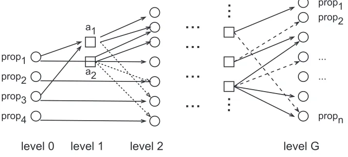
Starting from the initial state in the level 0, the planner will find all the possible actions

includingno-opactions (i.e. actions doing nothing) which have preconditions in level 0 to

construct the level 1. This means that level 2 contains all the propositions which could be

true as a result of applying all possible actions to the initial state. The process repeats to

construct the whole planning graph. Thus, the planning graph is a directed layered graph

which alternates between a level of propositions and a level of actions.

In the planning graph, each proposition level is a union of all possible states of that

level. The figure 2.6 below illustrates an example of a planning graph.

2.2.6.3 Mutual exclusion

With the construction of the planning graph described in the above section, a certain

level 0 level 1 level 2

...

... a1

a2

...

...

...

...

...

...

prop2 prop1

propn

level G

prop1 prop2 prop3 prop4

Figure 2.6: The overview of a planning graph

the algorithm stores states as a union of them, there might be two actions which cannot

hap-pen simultaneously due to a conflict in preconditions or effects. For example, an action may

delete preconditions of another action. Hence, not all the propositions of the proposition

level may be simultaneously true. Therefore, themutual exclusion relations, also called as

mutex relationsormutexes, are introduced to identify whether actions or propositions can

appear simultaneously.

Definition 2.6 Two actions a and b aremutexif:

• [Inference]either action deletes a precondition or an added effect of the other

ac-tions.

• [Competing needs] A precondition of a is logically inconsistent with a precondition

of b in the previous level.

Definition 2.7 Two proposition p and q are mutex if:

• All possible ways to create p are logically inconsistent with all possible ways to

create q.

2.2.6.4 Graphplan planner

The Graphplan planner [13] was introduce by Blum and Furst in 1995. It is an optimal

planner which finds an optimal solution (i.e. using the minimal steps) for classical planning

domains.

Graphplan contains two phases: the graph expansion and the solution extraction. In

the graph expansion, from the initial state, the planner applies possible actions and their

effects to advance the planning graph to the next level. The process is repeated until all

of the propositions of the goal state appear and are pairwise non-mutex. At this time,

the solution extraction is called to look for a solution in the planning graph. In the solution

extraction, starting from the propositions of the goal state, the planner looks for all possible

supporting actions and tries to add them into the plan. The preconditions of these selected

actions are then added. If it leads to a dead-end in the search tree, the planner will backtrack

and try other actions. The process continues to search backwards towards the initial state.

If it reaches the initial state, a solution is found and is optimal. At this time, the algorithm is

terminated. Otherwise, if all possible search branches have been tried, the graph expansion

is called again to advance the planning graph to the next level. If the planning graph has

levelled-off (i.e. the new level is the same as the previous one), there is no solution and the

algorithm stops.

The extension of Graphplan to deal with temporal planning is discussed in detail in

the next chapter. It describes the detail of the algorithms of TGP and TPSYS and the

improvements over Graphplan. Chapter 4 then describes in detail CPPlanner, which uses on

the planning graph to deal with temporal domains in which actions can have intermediate

2.2.7 Constraint Programming in planning

2.2.7.1 Introduction

Constraint programming is a very powerful approach to find an optimal solution. Encoding

the planning problems as CSPs [97, 22, 69, 68, 96] allows to use efficient built-in search

al-gorithms and techniques in Constraint Programming Solvers. Graphplan has been adapted

to use constraint programming [22, 68] and is a typical example to show that planning

problems can be encoded to CSPs and solved using CSP algorithms.

2.2.7.2 Constraint Satisfaction Problem

A constraint satisfaction problem is defined as P = (X, D, C), in which:

• X ={x1, x2, ..., xn}is a finite set of variables.

• D ={D1, D2, ..., Dn}is a set of finite domains for corresponding variables, xi ∈Di.

• C ={c1, c2, ..., cm}is a finite set of constraints.

Definition 2.8 A solutionto a CSP is an assignment of (v1, ..., vn), in which vi ∈Di, to

variables (x1, ..., xn) which satisfy all of the constraints in C.

For example, in Graphplan, the solution extraction process can be encoded as a dynamic

constraint satisfaction problem [22]. In this encoding, variables are propositions which

are looking for supporting actions. Thedomain for each variable consists of all possible

supporting actions of that proposition. The CSP starts with variables of all propositions

in the goal state. Each time new propositions appear which are preconditions of chosen

actions, new variables are created and added to the CSP. The CSP solver tries to look for

a possible assignment to variables. If there is a solution for the CSP problem, it is then

Constraint programming is successfully used for resource allocation and scheduling

problems. In AI Planning, applying constraint programming is still at the early stage.

However, it is a promising approach for AI planning, especially for optimal planning

sys-tems. Besides the above example of encoding the solution extraction of Graphplan into

CSP, there have been a few studies of applying constraint programming into AI Planning,

such as CPlan developed by Peter van Beek [97], Encoding Temporal Planning as CSP by

Mali [69], Generalizing GraphPlan by Formulating Planning as a CSP [68], and Utilizing

Structured Representations and CSPs in Conformant Probabilistic Planning [52].

2.3 Planning with time and resources

In classical planning, actions are assumed to have no duration. The actions can take place

instantaneously. However, this is unrealistic. In addition, resources are also considered in

real world problems. For instance, in order to fly from city A to city B, it will take durAB

time and consume fuelAB. With the ambition to deal with real world problems, temporal

planning and planning with resources have been introduced.

With the introduction of time into planning, actions can take place concurrently as long

as they are not in conflict with one another. Hence, the plan is now a sequence of actions

attached with their starting time. With time and resources, the expressivity of the problem

description increases, and so does the complexity. The search space becomes much bigger

comparing to that of the classical planning. The next sections will show an overview of

planning with time and resources.

2.3.1 Planning with time

2.3.1.1 Introduction

Unlike classical planning, in temporal planning, actions now have duration. This section

2.3.1.2 Temporal representation

According to the description of a temporal planning domain in the book [42], it has:

• constant symbolsare objects in the planning domains, such as cars, places, people.

• variable symbolsare eitherobject variablesthat are typed variables ortemporal

vari-ables.

• relation symbolsare either rigid relation symbolsrepresenting relations that do not

change during time, for example attach(crane, location), orflexible relation symbols

representing relations of the constants that may or may not hold at some instant for a

planning problem, for example at(car1, London).

• constraintsare eithertemporal constraintswhich reside within point algebra

calcu-lus, e.g. t1<t2, orbinding constraintson object variables, which are expressions of

the form x=y, x6=y and x∈D, with D being a set of constant symbols.

The rigid relations and binding constraints are object constraints, which are

time-invariant in this representation scheme.

Thetemporally qualified expressionis an expression in the form: ρ(ζ1,...,ζk)@[ts, te).

in which,ρis a flexible relation,ζiis a constant or object variable, and ts, teare temporal

variables, such that: ∀t∈[ts, te),ρ(ζ1,...,ζk) holds at t.

A temporal databaseis defined asφ = (F, C), in which F is a finite set of temporally

qualified expressions, and C is a finite set of temporal and object constraints.

Atemporal planning operator is a tuple o = (name(o), precond(o), effects(o), const(o),

in which:

• name(o) is in the form of o(x1, ..., xk, ts, te) such that o is the operator symbol, x1, ...,

• precond(o) and effects(o) are temporally qualified expressions.

• const(o) is a conjunction of temporal constraints and object constraints.

An action is an instance of the operator. The action a is applicable to φ=(F, C) iff

precond(a) is supported by F within some consistent constraints.

2.3.1.3 Approaches in temporal planning systems

This section describes a brief introduction to different approaches and techniques in

tem-poral planning, and illustrates temtem-poral planning systems. Chapter 3 will discuss in detail

these temporal planners.

Simple Temporal Constraint Problem (STP) and Temporal Constraint Network Problem

(TCSP), which were introduced by Dechter et al. [21], have been widely used in several

temporal planning systems [15, 51, 18], and many improvements have been introduced

[16].

In temporal state-space planning, planning systems have applied heuristics to guide the

search, such as TLplan [4], and later developments [5, 7, 3], TALplanner [24, 62, 61, 25],

and the HS planner [41].

In plan-space planning, ZENO planner [83] dealt with rich representations with variable

durations and linear constraints. It is one of the earliest planning systems which can deal

with complex planning domains including deadline goals, metric conditions and effects,

and continuous changes.

In the planning graph approach, TGP [89], TPSYS[38], and SAPA [23] deal with

du-rative actions. TGP and the early version of TPSYS extend the Graphplan planner to find

an optimal solution for temporal planning domains. SAPA applies a heuristic search based

on the planning graph.

In HTN planning, several planning systems, such as O-Plan [19], and SHOP2 [78] use

These approaches proved to successfully perform at the International Planning

Com-petition 2002. However, they make restrictive assumptions on actions, such as that actions

only have effects at the beginning or at the end of their execution.

2.3.2 Planning with resources

2.3.2.1 Introduction

Resources are an important part of making planning domains/problems more realistic.

However, since our main topic is working on temporal planning and planning systems,

planning with resources is not discussed in very detail. The section only gives an overview

of planning with resources.

In planning problems, resources can be categorized into two types: consumable

re-sources andreusableresources.

A consumable resource is consumed by an action during its execution. Fuel is a typical

example of a consumable resource. A reusable resource is used by an action during its

exe-cution; the resource is then released and unchanged when the action finishes. For example,

cars, locations are reusable resources.

Reusable resources are constraints on the number of actions which can perform in

par-allel, whereas consumable resources are constraints on whether the action can perform

freely during the lifespan of the plan.

Consumable resources are quantitative resources. These are encoded as a quantity with

a state. The value of this resource is often numeric. The consumption of this resource will

reduced its value accordingly. In some planning domains, there are actions which allow to

restore this resource. For example, an action drive(car, A, B) can consume an amount of

fuel. Another action refuel(car) can restore the fuel level for the car.

Reusable resources are qualitative resources. They are represented by the states of

objects. For example, when a robot arm is empty (or available), it means it is ready for

2.3.2.2 Approaches

There are several approaches to deal with planning domains with resources. In the work

of Srivistava and Kambhampati [94, 95], the authors tried to separate resources from

plan-ning. Resources are then managed and attached into the skeletal plan which is constructed

without resources earlier. The main difficulty of this idea is when the resource constraints

are too tight. In this case, it is very difficult to manage them into the skeletal plan. Because

of this difficulty, the attempt to separate resources from planning has been abandoned.

Many researchers have studied and implemented several planning systems to handle

resources. Penberthy and Weld [83] introduced ZENO planner, Laborie and Ghallab with

IxTeT [63], or Drabble and Tate with O-Plan [26], or Koehler’s work [58, 59] with

intro-duction of resources into the Graphplan framework. ZENO, IxTeT, and O-Plan are among

earliest planners which can handle planning domains with resources. However, due to the

limitation of the approaches they used at that time, their performance was not as good as

the current planning systems with new approaches.

The common idea in those systems is to consider resources as constraints and use

spe-cialized solvers to deal with these constraints. Dealing with resources makes planning

sim-ilar to scheduling. Systems, such as O-Plan and IxTeT, have used scheduling techniques to

solve the planning problems. O-Plan with optimistic and pessimistic resource profile, and

IxTeT identifying the minimum critical set of actions which have resource conflicts.

In ZENO, IxTeT, RealPlan and Koehler’s work, they also consider time as a resource.

ZENO and IxTeT used interval representation for actions and propositions, and applied

constraint programming techniques to manage the relationships between intervals. In

Re-alPlan and Koehler’s work, time is considered as steps, in which each corresponds to a set

2.4 Planning Domain Definition Language (PDDL)

2.4.1 Introduction

The Planning Domain Definition Language (PDDL) was introduced in order to help the

planning community to share planning models, problems and be able to compare their

systems. It became the standard language for the first International Planning Competition in

the community in 1998. Our planning system, CPPlanner, also uses PDDL as the language

for planning domains and problems. This section describes an overview of the language

and its development in the last few years.

Planning Domain Definition Language (PDDL) was first introduced by McDermott in

1998 with the purpose to make a standard planning language for the first International

Planning Competition. Since then, it has been accepted and widely used by the planning

community to share and exchange planning models. PDDL is an action-based planning

definition language, which was mainly inspired from the ideas of STRIPS. In the first

international planning competition in 1998, it was used as the standard definition language

for all participating planners. Before the introduction of PDDL, in the planning community,

each planning system used its own conventions on the input and output data. This caused

difficulty in comparing and sharing planning models. PDDL provides the standards for the

input and output data for planning systems. PDDL encourages scientists to develop and

compare the performance of their systems.

With the ambition to deal with realistic planning problems, PDDL has been extended

with more expressivity to describe more complex and realistic planning domains. In 2002,

it was extended to PDDL 2.1 which is able to model temporal planning domains and

do-mains with resources. In the international planning competition 2004, PDDL was extended

to PDDL 2.2, which added derived predicates and timed initial literals. Recently, Gerevini

and Long [40] extended it further by allowing to express strong and soft constraints on

plan trajectories (i.e. constraints over possible actions in the plan and intermediate states

constraints are ones attached with weights or values which are desired to be satisfied as

“much” as possible. They also proposed strong and soft problem goals (i.e. goals that must

be achieved in any valid plan, and goals that we desire to achieve, but that do not have to be

necessarily achieved). The following sections will introduce PDDL and its development.

2.4.2 PDDL

PDDL uses Lisp-like syntax to describe planning problems. It was built based on the

for-malisms of existing planning systems at that time, such as STRIPS [31], ADL [81], UCPOP

[82]. It is an action-centered language. PDDL separates planning domain descriptions

from problem descriptions. The planning domain description shows the general domain

behaviours via parameterised actions. The problem description contains initial state and

goal state of the problem. A planning problem is a pair of a domain description and a

problem description. Normally, one domain description can be paired with many problem

descriptions to create different planning problems in the same domain.

In the domain description, actions are described at an abstract level. In addition to

preconditions and effects, actions also have parameters which are assigned values when

the actions are applied. The preconditions and effects (i.e. post-conditions) are logical

propositions, objects and logical connectives.

Because PDDL is a general planning language, many planners just support a part of

it. In a domain description, requirements are introduced so that planning systems know

quickly whether they can handle it. Below are the most commonly-used requirements:

:strips

Description consists STRIPS only. :typing

Domains uses types. It is used to declare parameter and object types.

Some or all of the domain description

uses ADL syntax, e.g. actions have quantified and conditional effects, disjunctions and quantifiers in preconditions and goals. :equality

Domain uses "=" predicate as equality

In the original PDDL, the semantics is not formally described for the syntax proposed.

However, the language is widely accepted by the planning community. The language has

the power to express types of objects in planning domains, constrain types of arguments of

predicates, actions with negative preconditions or conditional effects etc. These expressive

abilities were fully described and proposed as ADL. It also attempted to form a standard

syntax for describing hierarchical domains which are used in HTN planners. However,

this attempt of proposing a standard syntax for hierarchical domains was not successfully

explored and was removed in PDDL 2.1. In addition, it also tried to propose a standard

syntax for numeric-valued fluents. However, in the planning competition in 1998 and even

2000, this part of the language is not applied.

Figure 2.7 shows a simple example of a domain description. This domain description

(define (domain gripper-strips) (:predicates (room ?r)

(ball ?b) (gripper ?g) (at-robby ?r) (at ?b ?r) (free ?g)

(carry ?o ?g)) ...

) )

(define (domain jug-pouring)

(:requirements :typing :fluents) (:types jug)

(:functors

(amount ?j -jug) (capacity ?j -jug)

-(fluent number)) (:action empty

:parameters (?jug1 ?jug2 - jug) :precondition (fluent-test

(>= (-(capacity ?jug2) (amount ?jug2)) (amount ?jug1))) :effect (and (change (amount ?jug1) 0)

(change (amount ?jug2)

(+ (amount ?jug1)(amount ?jug2))))) )

The example in the figure 2.8, shows how a planning system can tell from the domain’s

requirements whether or not it can handle the domain. For example, in the requirements of

the domain, the planner is required to handle fluents.

In PDDL, numbers are supported, and numeric quantities can be assigned and updated.

Figure 2.8 is also an example of numeric fluents used in PDDL. In this example, the water

is poured from jug1 to jug2 with the condition that jug2 is big enough to hold the water

from jug1. The effect of this action updates the quantities in each jug by a discrete

quan-tity. PDDL is also tweaked to handle resource consumption without using numeric fluents.

Figure 2.9 shows that the fuel is consumed by the car when it moves from one location to

(define (domain vehicle)

(:requirements :strips :typing)

(:types vehicle location fuel-level) (:predicates

(at ?v - vehicle ?p - location) (fuel ?v - vehicle ?f - fuel-level)

(accessible ?v - vehicle ?p1 ?p2 - location) (next ?f1 ?f2 - fuel-level))

(:action drive

:parameters (?v - vehicle ?from ?to - location ?fbefore ?fafter - fuel-level)

:precondition (and (at ?v ?from) (accessible ?v ?from ?to) (fuel ?v ?fbefore) (next ?fbefore ?fafter)) :effect (and (not (at ?v ?from))

(at ?v ?to)

(not (fuel ?v ?fbefore)) (fuel ?v ?fafter)))

)

Because of the complexity of PDDL, the first International Planning Competition in

1998, there were only 5 participants, in which three planners only supported STRIPS,

and the other two supported STRIPS/ADL. To encourage more participants, in the

sec-ond competition in 2000, the PDDL was restricted. In particular, negative precsec-onditions

were removed; parsing of ADL actions was simplified to avoid unnecessary “nesting”; and

objects were explicitly listed in the problems.

In short, the PDDL is the first planning language which is recognised and widely used

by the community. It helps the community to share planning problems, resources and

compare planning systems’ performance. However, the semantics need to be formally

defined. In addition, in order to encourage more people using PDDL as a standard language

for planning domains and problems, more structure, guidelines and supporting tools need

to be developed and introduced.

2.4.3 PDDL 2.1

PDDL 2.1 [37] was based on the original PDDL with the extension to allow numerical

vari-ables, and concurrent execution of durational actions. This extension was introduced in the

international planning competition in 2002. PDDL 2.1 has 5 levels, in which level 1 is

ADL planning, level 2 adds numerical variables, level 3 introduces discretised durative

ac-tions, and level 4 extends level 3 to allow continuous durative actions under certain restrict

assumptions. Finally, level 5, which is also known as PDDL+, removes the assumptions

and introduces processes and events allowing to model complex discrete and continuous

real-time systems. The higher the level is, the more expressive language is. However,

be-cause planning systems could not handle the complexities of level 4 and 5, only the first 3

levels were used in the planning competition in 2002. The syntax and semantics of the first

3 levels are formally defined in [37]. Level 4 and 5 were defined in [35].

CPPlanner, the system described in this thesis, deals with PDDL 2.1 level 3 with some

(define (domain jug-pouring)

(:requirements :typing :fluents) (:types jug)

(:functions

(amount ?j -jug) (capacity ?j -jug) (:action pour

:parameters (?jug1 ?jug2 - jug)

:precondition (>= (- (capacity ?jug2) (amount ?jug2)) (amount ?jug1)))

:effect (and (assign (amount ?jug1) 0) (change (amount ?jug2)

(increase (amount ?jug1)(amount ?jug2))))) )

Figure 2.10: Jug-pouring domain description, extracted from PDDL 2.1 document [37]

In PDDL 2.1, levels 1 and 2 have some minor modifications to the original PDDL

in order to simplify the parsing and the language. For example, instead of using change

to assign a numeric value to an object, PDDL 2.1 uses assign as direct assignment, and

increase and decrease as relative assignments, which makes the language clearer. The

declaration of functions is modified to allow only numeric-valued functions. PDDL2.1 has

functions in types ofobjects → R, whereas in original PDDL, functions are in types of

objects →object, allowingobjectto be extended by the application of functions to other

objects. With the consideration that numbers do not exist as independent objects in the

world but as attributes of objects, numeric expressions are only allowed as arguments to

predicates or values to action parameters.