Distributed Dynamic Clustering in Randomly
Deployed Wireless Sensor Networks
Lavanya Thunuguntla*, Rajendra Prasad G ** *Department of ECE, HITAM, Hyderabad, India ** Software Engineer, CA Technologies, Hyderabad, India
AbstractWireless Sensor networks (WSNs) present a new generation of real-time embedded systems that are being used in a wide variety of applications where traditional networking infrastructure is practically infeasible. However, WSNs have limited computation,energy and memory resources.Recent advances in wireless sensor networks have led to many new protocols specifically designed for sensor networks where energy awareness is an essential consideration. The goals of this paper is to study the various existing routing protocols such as hierarchical routing protocols, clustering methods and propose a new scheme, which enhances the lives of sensor nodes. we have proposed a novel Distributed Dynamic Clustering Algorithm in Randomly Deployed Wireless Sensor Networks. The key factors of our algorithm are optimizing the selection of cluster heads in which both energy of the nodes and total energy consumption of the cluster are considered, optimizing the number of nodes in the clusters according to the size of the network and the total power consumption of the cluster, breaking the clusters and reforming them to compensate the difference of the power consumption in different area, and finally re-clustering the clusters which have less number of nodes, by which we achieve energy efficiency in clustering. We conducted a comprehensive simulation and comparative study to evaluate the performance of the proposed clustering algorithm. Performance results show that our algorithm outperforms some of the existing clustering algorithms in terms of communication cost, energy consumption for clustering the network.
Key Words Sensor Nodes, Routing Protocol
I Introduction
Recent advances in micro-electro-mechanical systems (MEMS) and low power and highly integrated digital electronics have led to the development of micro sensors [1-5]. Such sensors are generally equipped with data processing and communication capabilities. The sensing circuitry measures ambient condition related to the environment surrounding the sensor and transforms them into an electrical signal. Processing such a signal reveals some properties about objects located and/or events happening in the vicinity of the sensor. The sensor sends such collected data, usually via radio transmitter, to a command center (sink) either directly or through a data concentration center (a gateway). The decrease in the size and cost of sensors, resulting from such technological advances, has fueled interest in the possible use of large set of disposable unattended sensors. Such interest has motivated intensive research in the past few years addressing the potential of collaboration among sensors in data gathering and processing and the coordination and managements of the sensing activity and data flow to the sink. A natural architecture for such collaborative distributed sensors is a network with wireless links that can be formed among the sensors in an ad hoc manner.
Networking unattended sensor nodes are expected to have significant impact on the efficiency of many military and civil applications such as combat field surveillance, security and disaster management. These systems process data gathered
from multiple sensors to monitor events in an area of interest. For example, in a disaster management’s setup, a large number of sensors can be dropped by a helicopter. Networking these sensors can assist rescue operations by locating survivors, identifying risky areas and making the rescue crew more aware of the overall situation. Such application of sensor networks not only increases the efficiency of rescue operations but also ensure the safety of the rescue crew. On the military side, applications of sensor networks are numerous. For example, the use of networked set of sensors can be limiting the need for personnel involvement in the usually dangerous reconnaissance missions. Security applications of sensor networks include intrusion detection and criminal hunting.
1.1 Constraints on Sensor Nodes
Sensor nodes are constrained in energy supply and bandwidth. Such constraints combined with a typical deployment of large number of sensor networks. These challenges necessitate energy-awareness at all layers of networking protocol stack. The issues related to physical and link layers are generally common for all kind of sensor applications, therefore the research on these areas has been focused on system-level power awareness such as dynamic voltage scaling, radio communication hardware, low duty cycle issues, system partitioning, energy aware MAC protocols. At the network layer, the main aim is to find ways for energy efficient route setup and reliable relaying of data from the sensor nodes to the sink so that the lifetime of the network in maximized. Routing in sensor networks is very challenging issue due to several characteristics that distinguish them from contemporary communication and wireless ad-hoc networks. First of all, it is not possible to build a global addressing scheme for the deployment of sheer number of sensor nodes. Therefore, classical IP-based protocol cannot be applied to sensor networks.Second, in contrary to typical communication networks almost all applications of sensor networks require the flow of sensed date from multiple regions (sources) to a particular sink.Third, generated data traffic has significant redundancy in it since multiple sensors may generate same data within the vicinity of a phenomenon. Such redundancy needs to be exploited by the routing protocols to improve energy and bandwidth utilization. Fourth, sensor nodes are generally tightly constrained in terms of transmission power, on-board energy, processing capacity and storage and thus require careful resource management.
II Sensor system Architecture
A. Network Dynamics: There are three main components in a sensor network. These are the sensor nodes, sink and monitored events. Aside from the very few setups that utilize mobile sensors [6], most of the network architectures assume that sensor nodes are stationary. On the other hand, supporting the mobility of sinks or cluster-heads (gateways) is sometimes deemed necessary [7]. Routing messages from or to moving nodes is more challenging since route stability becomes an important optimization factor, in addition to energy, bandwidth etc. The sensed event can be either dynamic or static depending on the application [8]. For instance, in a target detection/tracking application, the event (phenomenon) is dynamic whereas forest monitoring for early fire prevention is an example of static events. Monitoring static events allows the network to work in a reactive mode, simply generating traffic when reporting. Dynamic events in most applications require periodic reporting and consequently generate significant traffic to be routed to the sink.
B. Node Deployment: Another consideration is the topological deployment of nodes. This is application dependent and affects the performance of the routing protocol. The deployment is either deterministic or self-organizing. In deterministic situations, the sensors are manually placed and data is routed through pre-determined paths. However in self-organizing systems, the sensor nodes are scattered randomly creating an infrastructure in an ad hoc manner [2]. In that infrastructure, the position of the sink or the cluster-head is also crucial in terms of energy efficiency and performance. When the distribution of nodes is not uniform, optimal clustering becomes a pressing issue to enable energy efficient network operation.
C. Energy Considerations: During the creation of an infrastructure, the process of setting up the routes is greatly influenced by energy considerations. Since the transmission power of a wireless radio is proportional to distance squared or even higher order in the presence of obstacles, multi-hop routing will consume less energy than direct communication. However, multi-hop routing introduces significant overhead for topology management and medium access control. Direct routing would perform well enough if all the nodes were very close to the sink [8]. Most of the time sensors are scattered randomly over an area of interest and multi-hop routing becomes unavoidable.
D. Data Delivery Models: Depending on the application of the sensor network, the data delivery model to the sink can be continuous, event-driven, query-driven and hybrid [8]. In the continuous delivery model, each sensor sends data periodically. In event-driven and query-driven models, the transmission of data is triggered when an event occurs or a query is generated by the sink. Some networks apply a hybrid model using a combination of continuous, event-driven and query-driven data delivery. The routing protocol is highly influenced by the data delivery model, especially with regard to the minimization of energy consumption and route stability. For instance, hierarchical routing protocol is the most efficient alternative for a habitat monitoring applications where data is continuously transmitted to the sink. This is due to the fact that such an application generates significant redundant data that can be aggregated on route to the sink, thus reducing traffic and saving energy.
E. Node Capabilities: In a sensor network, different functionalities can be associated with the sensor nodes. In
earlier all sensor nodes are assumed to be homogenous, having equal capacity in terms of computation, communication and power. However, depending on the application a node can be dedicated to a particular special function such as relaying, sensing and aggregation since engaging the three functionalities at the same time on a node might quickly drain the energy of that node. Some of the hierarchical protocols proposed in the literature designate a cluster-head different from the normal sensors. While some networks have picked cluster-heads from the deployed sensors [9], in other applications a cluster head is more powerful than the sensor nodes in terms of energy, bandwidth and memory. In such cases, the burden of transmission to the sink and aggregation is handled by the cluster-head. Inclusion of heterogeneous set of sensors raises multiple technical issues related to data routing. For instance, some applications might require a diverse mixture of sensors for monitoring temperature, pressure and humidity of the surrounding environment, detecting motion via acoustic signatures and capturing the image or video tracking of moving objects. These special sensors either deployed independently or the functionality can be included on the normal sensors to be used on demand. Reading generated from these sensors can be at different rates, subject to diverse quality of service constraints and following multiple data delivery models, as explained earlier. Therefore, such a heterogeneous environment makes data routing more challenging.
F. Data Aggregation/Fusion: Since sensor nodes might generate significant redundant data, similar packets from multiple nodes can be aggregated so that the number of transmissions would be reduced. Data aggregation is the combination of data from different sources by using functions such as suppression (eliminating duplicates), min, max and average [9]. Some of these functions can be performed either partially or fully in each sensor node, by allowing sensor nodes to conduct in-network data reduction. Recognizing that computation would be less energy consuming than communication, substantial energy savings can be obtained through data aggregation. This technique has been used to achieve energy efficiency and traffic optimization in a number of routing protocols. In some network architectures, all aggregation functions are assigned to more powerful and specialized nodes. Data aggregation is also feasible through signal processing techniques. In that case, it is referred as data fusion where a node is capable of producing a more accurate signal by reducing the noise and using some techniques such as beam forming to combine the signals.
III Overview of IEEE 802.15.4 and Routing Protocols in Sensor Networks
3.1 IEEE 802.15.4
self-configuring, multi-hop network. A device in an 802.15.4 network can use either a 64-bit IEEE address or a 16-bit short address assigned during the association procedure, and a single 802.15.4 network can accommodate up to 64k (216) devices. Wireless links under 802.15.4 can operate in three license free industrial scientific medical (ISM) frequency bands. These accommodate over air data rates of 250 kb/sec (or expressed in symbols, (62.5 ksym/sec) in the 2.4 GHz band, 40 kb/sec (40 ksym/sec) in the 915 MHz band and 20 kb/sec (20 ksym/sec) in the 868 MHz. Total 27 channels are allocated in 802.15.4, with 16 channels in the 2.4 GHz band, 10 channels in the 915 MHz band, and 1 channel in the 868 MHz band.
3.2 Routing Protocols in Sensor Networks
Sensor network nodes are often limited in battery capacity and processing power. Thus, it is imperative to develop solutions that are both energy and computationally efficient. Energy aware routing in sensor networks has received significant attention in recent years. Finding a good routing algorithm to prolong the network lifetime is an important problem, since sensor nodes are usually quite limited in battery capacity and processing power. For exactly the same reason, complex routing algorithms do not work well in this scenario, due to excessive overhead.
The ease of deployment, ad hoc connectivity and cost-effectiveness of a wireless sensor network are revolutionizing remote monitoring applications. At the node level, data communication is the dominant component of energy consumption, and protocol design for sensor networks is geared towards reducing data traffic in the network. As sensors close to the event being monitored sense similar data, the focus of existing research has been to aggregate (combine, partially compute and compress) sensor data at a local level before transmitting it to a remote user called the sink. The number of nodes that sense attributes related to an event in a geographical region depends on the footprint of the event. 3.3 Performance Metrics
We define the following metrics for studying the performance of 802.15.4. All metrics are defined with respect to MAC sub layer and PHY layer in order to isolate the effects of MAC and PHY from those of upper layers.
• Packet delivery ratio: The ratio of packets successfully received to packets sent in MAC sub layer. This metric does not differentiate transmissions and retransmissions, and therefore does not reflect what percentage of upper layer payload is successfully delivered, although they are related. • Hop delay: The transaction time of passing a packet to a one-hop neighbor, including time of all necessary processing, back off as well as transmission, and averaged over all successful end-to-end transmissions within a simulation run. It is not only used for measuring packet delivery latency, but also used as a negative indicator of the MAC sub layer capacity. The MAC sub layer has to handle the packets one by one and therefore a long delay means a small capacity. • Successful association rate: The ratio of devices successfully associated with a coordinator to the total devices trying to associate with a coordinator. In our experiments, a device will retry in one second if it fails to associate with a coordinator in the previous attempt. The association is considered successful if a device is able to associate with a coordinator during a simulation run, even if multiple association attempts have been made.
• Association efficiency: The average number of attempts per successful association.
• Orphaning rate: A device is considered orphaned if it misses aMaxLostBeacons (default value 4) beacons from its coordinator in a row. The orphaning rate is defined as the ratio of devices orphaned at least once to the total devices that are in beacon enabled mode and keep tracking beacons. This metric is not applicable to devices in non-beacon enabled mode or devices in beacon enabled mode but not tracking beacons. In our experiments, all devices in beacon enabled mode track beacons.
• Orphaning recovery rate: Two different versions are defined for this metric. One is the ratio of orphaned devices that have successfully relocated their coordinators, i.e., have recovered from orphaning, to the total orphaned devices. The other is the ratio of recovered orphanings to the total orphanings, in which multiple orphanings of a device are counted. No further attempt is made if the orphaning recovery procedure fails. • Collision rate: The total collisions during a simulation run. • Collision rate between hidden terminals: The total collisions that occur between hidden terminals during a simulation run. Hidden terminals prevent carrier sense from working effectively, and therefore transmissions from them are likely to collide at a third node. In 802.11, the request-to-send (RTS) and clear-to-send (CTS) mechanism is used to tackle this problem.
• Repeated collision rate: The total collisions that happen more than once between the same pair of packets during a simulation runs.
• Collision distribution: The time distribution, within a super frame, of collisions. This metric is only used in beacon enabled mode.
• Duty cycle: The ratio of the active duration, including transmission, reception and carrier sense time, of a transceiver to the whole session duration.
Time to first node to die: When the first node runs out of energy, the network within the cluster is said to be partitioned. The name network partitioning reflects the fact that some routes become invalid and cluster-wide rerouting may be immanent.
Average lifetime of a node: This gives a good measure of the network lifetime. A routing algorithm, which maximizes the lifetime of the network, is desirable. This metric also shows how efficient is the algorithm in energy consumption.
Average delay per packet: Defined as the average time a packet takes from a sensor node to the gateway. Most energy aware routing algorithms try to minimize the consumed energy. However, the applications that deal with real-time data is delay sensitive, so this metric is important in our case.
Network Throughput: Defined as the total number of data packets received at the gateway divided by the simulation time. The throughput for both real-time and non-real-time traffic will be considered independently.
IV Proposed Algorithm for Clustering the Sensor Nodes 4.1 Objectives of Algorithm
The objectives when designing the clustering algorithm were the following:
1. The algorithm must be distributed, since every node in the network only has local knowledge.
clusters where a node always is directly connected to the cluster head normally have a time complexity of O (1). The Max-Min D-cluster algorithm have a time complexity of O(d), where no node is more than d hops away from the cluster head. The algorithm presented here has a time complexity of O (d2), where no node is more than d hops away from the cluster head. Since d is likely to be very small (probably no more than 3), this is an acceptable complexity. 3. The created clusters should be reasonably efficient, that is, the selected cluster heads should cover a large number of nodes. If the clustering structure becomes too complex (too many clusters), the number of messages needed to maintain the routing structure would cause congestion in the network. Since the algorithm presented in this paper makes it possible to create clusters with a radius larger than 1, it is possible to create relatively large clusters. At the same time, there should be a mechanism to prevent the clusters from growing too large. If the clusters grow too large, the load on the cluster head, that is responsible for the routing inside the cluster, becomes too large. The Max-Min D-cluster algorithm creates clusters with a given radius, but there is no way to limit the maximum cluster size.
4. A maintenance function should be used to split large clusters and direct new nodes to join existing clusters. Most existing clustering algorithms create new clustering structures from scratch after a specified time interval. The Max-Min D-cluster performs maintenance until the D-clustering structure has degraded, that is, until the number of clusters has grown too large. The goal for the work presented in this paper is to present a clustering algorithm that does not have to rely on reclustering at all. This is because the maintenance part of the clustering algorithm should require less communication overhead.
VDescription of Algorithm
STEP 1: Each node finds and stores the neighbor nodes that are the nodes which are in its communication range.
STEP 2: Each node broadcasts the list of nodes that it can hear, that is, the set of nodes that are within the communication range of the original node. If a node A hears from a node B with a higher number of neighbors than itself, node A sends a message to B requesting to join B’s cluster. If B already has resigned as a cluster head itself, B returns a rejection, otherwise B returns a confirmation. When A receives the confirmation, A resigns as a cluster head. Another possibility is that the cluster with node B as cluster head has already reached maximum size or its energy level is very low. In this case, all requests are automatically met with rejection. If the cluster would be allowed to grow too large, the cluster head’s power supply would soon be depleted since the routing would take too many resources.
STEP 3: When the previous step is completed, the entire network is divided into a number of clusters. Each node belongs to exactly one cluster, and a node is either a cluster head or directly connected to one. The next step is that every cluster broadcasts its size to all neighboring nodes. If a node receives a message from a cluster that has a larger size than the cluster it currently belongs to, it joins the new cluster instead. It sends notifications to both the new and the old cluster to update them about its new status. This assumes that the larger cluster has not reached the maximum size yet. The notifications first go to the cluster heads, and are then
propagated to the entire cluster. This process can be repeated several times, depending on what the maximum cluster diameter is considered to be in this case. Each node keeps track of the id of its cluster head, the first step in the path to its cluster head, the distance to the cluster head, the time the node has been a member of its current cluster, as well as the number of nodes in the cluster. A cluster head also keeps track of the time each node in its cluster has been a member of that cluster.
STEP 4: It is possible for a cluster to grow too large. Consider a situation when a cluster is just below the maximum allowed size, and several nodes join simultaneously. Eventually, the cluster head will be notified of all the new nodes. Since the size of the cluster exceeds the maximum allowed size, one or several nodes need to be disconnected from the cluster. Based on the assumption that some nodes move in groups, the nodes that have been members of the cluster for a long time are the nodes that are most likely to stay in the vicinity of the cluster head. This means that the nodes that have been with the cluster for the shortest amount of time should be the first to leave the cluster when it grows too large.
STEP 5: A node can leave a cluster, either because the situation described above, or because it is moving away from the cluster. Even if it loses contact with the node that is the first step to the cluster head, it might still be able to connect to another node in the cluster. However, if the node is more than d hops away from the cluster head, it must leave that cluster. When a node leaves a cluster, it tries to find another cluster to connect to. That cluster must be smaller than the maximum allowed size, and the node cannot be more than d hops away from the cluster head. If several such clusters are found, the node joins the largest one. If no such cluster is found, the node forms a cluster with itself as cluster head and only member.
VI Simulation and Results
We have implemented our algorithm in C–language under Linux environment. Every node in the network belongs to some cluster, if a cluster has a single node we call it as orphan node.
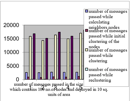
0 5000 10000 15000 20000
1 2 3 4 5
number of messages passed in the size of network which contains 100 no.of nodes and deployed in 10 sq.
units of area
number of messages passed while calculating neighbors nodes number of messages passed while initial clustering of the nodes
number of messages passed while clustering
number of messages passed while reclustering
0 100000 200000
1 2 3 4 5
number of message passed in the size of network which contains 500 no. of nodes
and deployed in 25 square units of area
number of messages passed while calculating neighbors nodes
Fig 6.2 No. of messages passed in the size of network which contains 500 no.of nodes and deployed in 25 sq. units of area
0 50000
1 2 3
number of messages passed in the network which contains 100 no. of nodes and deployed
in different units of area
number of messages passed while calculating neighbors nodes
Fig 6.3 No. of messages passed in the size of network which contains 100 no.of nodes and deployed in different units of area
0 100000 200000
1 2 3
number of messages passed in the network which contains 500 no. of nodes and deployed
in different units of area 25,30and 35
number of messages passed while calculating neighbors nodes
Fig 6.4 No. of messages passed in the size of network which contains 500 no.of nodes and deployed in different units of area
25,30,35
0 5000 10000
1 2 3 4 5
energy comsumed in the size of network which contains 100 no.of nodes and deployed in 10
sq. units of area
network energy before clustering
Fig 6.5 Energy consumed in the size of network contains 100 no.of nodes and deployed in 10 sq. units of area
0 20000 40000
1 2 3 4 5
energy cconsumed in the size of network which contains 500 no.of nodes and
deployed in 25 sq. units of area
network energy before clustering
Fig 6.6 Energy consumed in the size of network contains 500 no.of nodes and deployed in 25 sq. units of area
0 2000 4000 6000 8000
1 2 3
energy consumed in the network which contains 100 no. of nodes and
deployed in different units of area
network energy before clustering
Fig 6.7 Energy consumed in the size of network contains 100 no.of nodes and deployed in different units of area
0
20000
40000
1
2
3
energy consumed in the network which contains 500 no. of nodes and
deployed in different units of area
network energy before clustering
Fig 6.8 Energy consumed in the size of network which contains 500 no.of nodes and deployed different units of area
It can be observed from the above graphs that if the nodes deployed in large area then the communication cost will be decreasing and at the same time the consumption of energy increases.
VII Conclusion and Future Work
we have proposed our method for clustering the scattered distribution of sensor nodes and we worked out some examples on it. We implemented the algorithm and simulated it for various parameters.We have developed a novel algorithm for clustering the sensor network. We can use this algorithm for implementing a power aware routing protocol for sensor networks.
References
[1] I. F. Akyildiz et al., “Wireless sensor networks: a survey”, Computer
Networks, Vol. 38, pp. 393 - 422, March 2002.
[2] K. Sohrabi, et al., "Protocols for self-organization of a wireless sensor network,” IEEE Personal Communications, Vol. 7, No. 5, pp. 16-27,
October 2000.
[3] R. Min, et al., "Low Power Wireless Sensor Networks", in the
Proceedings of International Conference on VLSI Design, Bangalore,
India, January 2001.
[4] J.M. Rabaey, et al., "PicoRadio supports ad hoc ultra low power wireless networking," IEEE Computer, Vol. 33, pp. 42-48, July 2000.
[5] R. H. Katz, J. M. Kahn and K. S. J. Pister, “Mobile Networking for Smart Dust,” in the Proceedings of the 5th Annual ACM/IEEE International Conference on Mobile Computing and Networking (MobiCom’99),
Seattle, WA, August 1999.
[6] L. Subramanian and R. H. Katz, "An Architecture for Building Self Configurable Systems," in the Proceedings of IEEE/ACM Workshop on
[7] F. Ye et al., “A Two-tier Data Dissemination Model for Large-scale Wireless Sensor Networks,” in the Proceedings of Mobicom’02, Atlanta, GA, Septmeber, 2002.
[8] S. Tilak et al., “A Taxonomy of Wireless Microsensor Network Models,”
in ACM Mobile Computing and Communications Review (MC2R), June
2002.
[9] Kemal Akkaya, Mohamed F. Younis. “A survey on routing protocols for wireless sensor networks”, Ad Hoc Networks vol 3(3), page. 325-349, 2005.
Authors
MsLavanya Thunuguntla has 6 years of Teaching experience and presently working as an Associate Professor in the Department of ECE in Hyderabad Institute of Technology and Management (HITAM), Hyderabad, AP(India).She received her B.Sc degree in Computer Science from Acharya Nagarjuna University in 2002, M.Sc degree in Physics from University of Hyderabad, Hyderabad in 2004 and M.Tech from Indian Institute of Technology (IIT) Kharagpur in 2007. She has Professional Membership in IEEE. She has various journal publications in International journals in the field of Nano Technology etc. She has guided several M.Tech and B.Tech projects. She has strong motivation towards research in the fields of Nano Technology, Microwave and Optical & Analog Communications ,VLSI system design etc.