Sensor Network for In-Situ Failure Identification in Woven Composites after Impact Events.

(1)

ABSTRACT

GARRETT, RYAN CHARLES. Sensor Network for In-Situ Failure Identification in Woven Composites after Impact Events. (Under the direction of Kara J. Peters.)

(2)

SENSOR NETWORK FOR IN-SITU FAILURE IDENTIFICATION IN WOVEN COMPOSITES AFTER IMPACT EVENTS

by

RYAN CHARLES GARRETT

A thesis submitted to the Graduate Faculty of North Carolina State University

in partial fulfillment of the requirements for the Degree of

Master of Science

MECHANICAL ENGINEERING

Raleigh, North Carolina 2007

APPROVED BY:

_________________________ _________________________ Dr. Mohammed Zikry Dr. Eric Klang

________________________________ Dr. Kara Peters

(3)

BIOGRAPHY

Ryan Garrett was born in Greenville, N.C. on August 19, 1983 to Matt and Becky Garrett. He has a brother, Steven, who is two and a half years older and a sister, Emily, who is a year and a half younger. Ryan spent most of his childhood and teenage years in the town of Sanford, N.C. Ryan attended J.R. Ingram, Jr. Elementary school and Lee Christian school for all of middle and high school. He played varsity soccer and basketball. Ryan graduated high school as class valedictorian and received the prestigious Park Scholarship at North Carolina State University.

Ryan majored in mechanical engineering and was active with a variety of organizations, including Grace Community Church, Phi Sigma Pi, and the Order of 30&3, serving as vice president for two years. Ryan studied abroad in Spain during the summer of 2003. He was inducted into Phi Kappa Phi in 2004. As a junior, he was accepted into the Accelerated B.S./M.S. degree program in mechanical engineering. Ryan finished his bachelor’s degree in May 2006 and graduated valedictorian with a 4.00 GPA. In July 2006 Ryan married his wife Candice, whom he met as a freshman at North Carolina State University.

(4)

ACKNOWLEDGEMENTS

Ryan wishes to express his gratitude and appreciation to his advisor, Dr. Kara Peters, both for her guidance and assistance, and also the independence to take the topic in directions of personal interest. Ryan also thanks also Dr. Eric Klang and Dr. Mohammed Zikry, members of the advisory committee.

Ryan would like to acknowledge the support of the National Science Foundation through grant CMS 0219690, the National Defense Science and Engineering Graduate Fellowship program, and the North Carolina Space Grant Consortium.

Ryan personally thanks Joe Seawell, Brad Armstrong, Sharon Kiesel, Guoliang Jiang, and Dr. Peters for their help in setting up and conducting experiments. Ryan further thanks Wayne Zimmerman of Loctite Corporation, and Advanced Composites Group for the donation of supplies.

Ryan would like to thank Roberto Garcia of the NCSU Analytical Instrumentation Facility for help with optical microscopy, and Skip Richardson and Mike Breedlove of the NCSU machine shop in the Department of Mechanical and Aerospace Engineering, for their help in machining the components needed for this study.

(5)

TABLE OF CONTENTS PAGE

List of Tables……….. v

List of Figures………. vi

Chapter 1. Introduction and Literature Review……… 1

Chapter 2. Experimental Methods……….. 8

Chapter 3. Experimental Results……….23

Chapter 4. Conclusion and Future Work………... 43

References………... 45

(6)

LIST OF TABLES PAGE Table 2.1. Composite specimen descriptions………. 17 Table 3.1. Impact data summary for specimens C1-C6………. 31 Table 3.2. Mean and standard deviation of physical parameters

for specimens C1-C6………... 31 Table 3.3. Light transmission test data………... 31 Table 3.4. Impact event results for composite specimens

(7)

LIST OF FIGURES PAGE

Figure 1.1. Fiber Bragg Grating schematic……… 7

Figure 1.2. FBG sensors serially multiplexed……… 7

Figure 2.1. Temperature cure cycle for specimen fabrication………... 15

Figure 2.2. Fiber jig and composite mold in place prior to final cure cycle……… 15

Figure 2.3. Composite specimen configurations for (a) uni-directional embedment of optical fibers and (b) bi-directional embedment of optical fibers………....…... 16

Figure 2.4. Specimen with high density (6.3 OF/cm) of embedded optical fibers……….. 17

Figure 2.5. Instrumented drop tower facility (Pearson, 2005)………... 18

Figure 2.6. Support/clamp system for securing specimens for impact (Pearson, 2005)………....19

Figure 2.7. Specimen dimensions and impact location……….. 20

Figure 2.8. Perforation of specimen C1………. 20

Figure 2.9. Specimen C15, shown mounted in impact tower, with FBG sensors spliced together and connected in series………... 21

Figure 2.10. “Resin eye” effect………. 21

Figure 2.11. Microscopy image of cross-section with minimum embedded fiber density, 0.79 optical fibers/cm………. 22

Figure 2.12. Microscopy image of cross-section with maximum embedded fiber density, 6.3 optical fibers/cm………... 22

Figure 3.1. Contact force per strike for specimen C1……… 30

Figure 3.2. Dissipated energy per strike for specimen C1………. 30

Figure 3.3. Specimen C7, pre-impact photo with no embedded optical fibers……….. 32

Figure 3.4. Voids caused by lack of pressure during cure cycle in specimen C11……… 33

Figure 3.5. In specimen C11 delamination is clearly seen at the optical fiber embedment layer……… 33

Figure 3.6. Contact force per strike for specimen C9……… 34

Figure 3.7. Dissipated energy per strike for specimen C9………. 34

Figure 3.8. Total dissipated energy in each tested specimen………. 35

Figure 3.9. Maximum contact force in each tested specimen……… 35

Figure 3.10. Dissipated energy per strike for each tested specimen………….. 36

Figure 3.11. Number of strikes to failure for each tested specimen………….. 36

Figure 3.12. Dissipated Energy trend line for (a) typical failure and (b) delamination failure of C11………... 37

Figure 3.13. Pre-embedment, pre-impact spectral response of eight FBG sensors embedded into C15………... 38

(8)

PAGE Figure 3.15. FBG sensor locations within single quadrant

of specimen C15………. 40

Figure 3.16. Fabrication photos for specimen C15. ………. 41

Figure 3.17. Completed specimen C15 ………. 42

Figure 3.18. Normalized transmitted intensity after each impact for sensor #1 (080705770009)……… 43

Figure 3.19. Normalized transmitted intensity after each impact for sensor #8 (080705770030)……… 43

Figure 3.20. Micro-strain by strike for sensor #3 (08070577015)………. 44

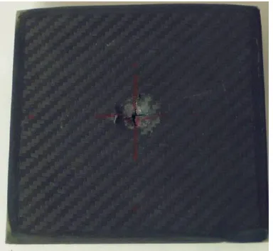
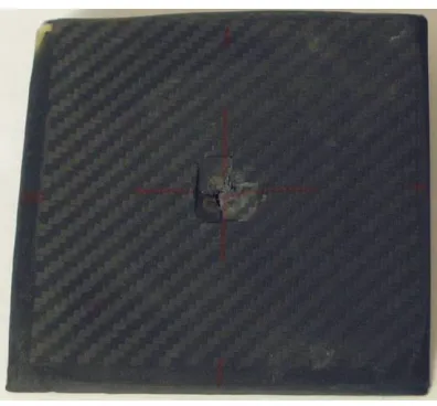
Figure A.1. Post impact perforation for specimen (a) C2, (b) C3………... 49

Figure A.2. Post impact perforation for specimen (a) C4, (b) C5………... 50

Figure A.3. Post impact perforation for specimen C6………... 51

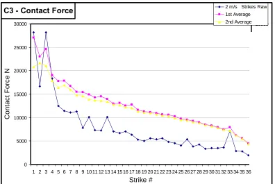
Figure A.4. Contact force for specimen C2………... 52

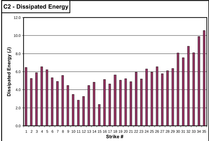
Figure A.5. Dissipated energy for specimen C2……… 52

Figure A.6. Contact force for specimen C3……… 53

Figure A.7. Dissipated energy for specimen C3………. 53

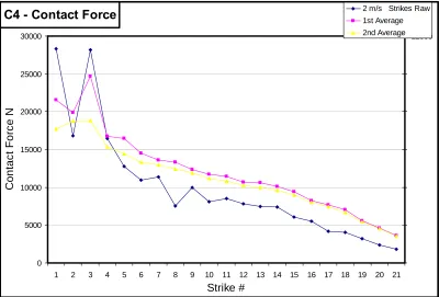
Figure A.8. Contact force for specimen C4……… 54

Figure A.9. Dissipated energy for specimen C4………. 54

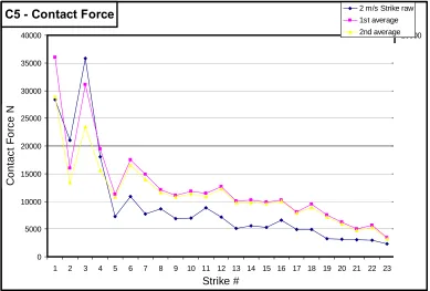
Figure A.10. Contact force for specimen C5……….. 55

Figure A.11. Dissipated energy for specimen C5………... 55

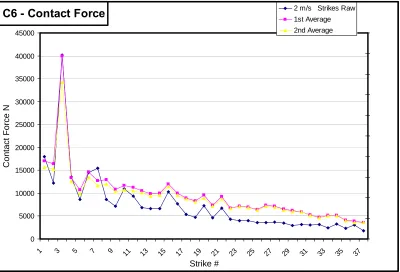
Figure A.12. Contact force for specimen C6……….. 56

Figure A.13. Dissipated energy for specimen C6………... 56

Figure A.14. Contact force per strike for specimen C10………... 57

Figure A.15. Dissipated energy per strike for specimen C10……… 57

Figure A.16. Contact force per strike for specimen C11……… 58

Figure A.22. Spectral response of FBG #1 080705770009………61

Figure A.30. Normalized transmitted intensity per strike for sensor #2 (080705770012)………. …….. 65

(9)

PAGE Figure A.32. Normalized transmitted intensity per strike

for sensor #4 (080705770012)……… 66

Figure A.33. Normalized transmitted intensity per strike for sensor #5 (080705770012)……… 66

Figure A.36. Strain by strike for sensor #1 (08070577009)……….. 68

(10)

CHAPTER 1. INTRODUCTION AND LITERATURE REVIEW

Overview

This study investigates the development of a fiber Bragg grating (FBG) optical sensor network to measure and monitor damage in a composite material induced by low velocity impact events occurring at a single location. The effects of the embedded optical fibers on the host material and their interaction with each other are first considered on both a micro- and macro-mechanics scale. The mechanical low-velocity impact response of two-dimensional woven composite laminates with and without various densities of embedded optical fibers is therefore investigated. Modifications to the specimen fabrication process are then developed to facilitate the embedment of a large density of optical fibers. The light transmission capabilities of embedded optical fibers are also studied to determine if the current fabrication processes permits sufficient light transmission to allow interrogation of the embedded FBG sensor network. A FBG sensor network is finally embedded in a composite sample which is then subjected to multiple low velocity impacts events while sensor data is captured after each impact event until complete failure of the composite material system. The FBG sensor data is evaluated to determine the ability of the chosen sensor configuration to measure strain at various points within the sample for the purpose of quantifying the progression of damage and differentiating between multiple forms of damage.

(11)

microscopic evaluation. Chapter 3 details the experimental results and the performance of the sensor network during impact events. Chapter 4 presents the conclusions derived from this study and proposes future work topics in this research area.

Damage in Woven Composite Laminates

(12)

Previous studies have investigated the use of a single embedded FBG for damage initiation and progression monitoring in a two-dimensional woven composite during multiple low velocity impact events. Pearson, et al. (2007), and Tsutsui et al. (2004) demonstrated the

use of embedded FBG sensors to detect impact damage in laminated and stiffened composite panels. Similar studies have focused on impact damage in fiber metal laminates (Kuang et

al., 2001). Each of these studies demonstrate that FBG sensors can provide detailed

information about the state of strain within the composite material system. In particular, as the strain along the grating becomes non-uniform, the complicated spectral response of the FBG can provide quantitative information on the strain field, more than simply the average strain value.

For a general application, the proper placement of the FBG sensors would require a reasonable knowledge of potential impact locations. On the other hand, the development of a network of sensing FBGs would allow for damage monitoring over a given area without knowing a-priori the location of impact events. A sensing network could also provide detailed information on the form, mechanisms, severity and progression of damage by providing spatial information.

Fiber Bragg Gratings

(13)

multiplexed together for distributed sensing, and therefore can be used for large- and small-scale applications. Optical sensors in general demonstrate excellent durability and often a working life of twenty-five years or more. Additionally, optical sensors are extremely lightweight, making them advantageous for many aerospace applications. Although the sensors themselves, as well as the required equipment, are expensive, this technology is becoming more affordable as production technology improves.

Fiber Bragg Gratings were first created by Hill et al. (1978). Fiber Bragg gratings are

periodic modulations in the effective index of refraction of an optical fiber core. This modulation is produced by exposing the core of an optical fiber to a strong UV-laser light interference pattern, producing permanent gratings. At the Bragg wavelength, λ_B,

constructive interference occurs between the multiple reflected lightwaves as each reflection is in phase with the others. At this wavelength, a resonance conditions occurs in reflection and the lightwave is reflected rather than transmitted through the grating. The resonance condition occurs at the wavelength,

2

B neff

λ = Λ (1.1)

where neff is the effective index of refraction of the optical fiber for the fundamental mode

and Λ is the period of the Bragg grating (see Figure 1.1).

(14)

(

)

(

)

2

12 11 12

1 2

eff

B e

n

p p p 1 p _B

λ ⎧⎪ ⎡ ν ⎤⎫⎪ελ

Δ =_⎨ − _⎣ − + _⎦_⎬ = −

⎪ ⎪

⎩ ⎭

ελ (1.2)

where ν is the Poisson’s ratio and p11 and p12 are the photoelastic constants of the optical

fiber material. For fused silica fibers, a typical of pe is 0.78. For non-uniform strain applied

along the FBG, numerous wavelengths will be reflected at various intensities.

FBG sensors are also very sensitive to temperature changes. In applications where temperature variations will be present, one option is to incorporate a reference grating which will only measure strain due to temperature change. This allows for the temperature

dependence to be eliminated from consideration.

FBGs can be multiplexed together to permit distributed sensing. FBGs of slightly different Bragg wavelengths may be spliced together serially to create a sensing network requiring just a single light source (see Figure 1.2). This technique is known as wavelength division multiplexing and will be applied in this study. Because FBG sensor measurements are interpreted from wavelength shifts rather than intensity changes, splice losses generally do not limit the capability of FBG sensing networks.

Embedment of FBGs in Composite Materials

(15)

that no fibers outside of the damage area fractured. This study was able to measure initial damage but had very limited ability to monitor the progression of damage. Their results showed that the presence of the optical fiber network did not deteriorate the damage response of the composite. However, slight weakening can occur during tensile loading and moderate to extreme weakening has been recorded in compression tests with large quantities of embedded fibers (Jenson and Pascual, 1990; Jenson et al., 1991). The orientation of the

embedded optical fibers relative to the host fibers significantly affects to what degree the composite compressive strength is degraded (Mall et al., 1996; Jensen et al., 1991).

(16)

CHAPTER 1 FIGURES

Figure 1.1. Fiber Bragg Grating schematic.

(17)

CHAPTER 2. EXPERIMENTAL METHODS

Specimen Preparation

Two-dimensional 2x2 twill woven carbon fiber prepreg with thermoset epoxy matrix was obtained from the Advanced Composite Group and used for all specimens in this study. The prepreg is essentially isotropic in the plane of the woven fiber. Each composite specimen was fashioned into 127 mm square coupons, composed of twenty-four laminae of the woven carbon fiber prepreg, resulting in an overall thickness of 4 mm. The prepreg layers were placed in a 127 mm square metal mold that had been lubricated with carnauba wax and mold releaser agent to allow easy removal of the cured specimen. The carbon fiber prepreg layers were then sealed in a vacuum bag and a vacuum was drawn to remove air voids between the laminae. The entire setup was then cured in a hotpress at a constant pressure of 1.38 MPa and varying temperature cycle, as shown in Figure 2.1.

(18)

fibers to the jig. A UV lamp operating at a 365 nm wavelength was used to cure the glue to firmly hold the fibers in place.

(19)

top (Figure 2.3b). Each of these techniques produced a final twenty-four layer composite. The details of each specimen’s layup and optical fiber density are shown in Table 2.1.

Light Transmission Testing

Each of the embedded optical fibers was tested post specimen manufacturing for total light transmission. Light transmission testing was performed for the preliminary specimens to ensure that the fabrication technique was suitable, meaning that the technique consistently produced embedded sensors with sufficient light transmission. As explained earlier, FBG sensors measure strain based on resonant wavelengths, not intensity at a particular wavelength. Therefore, transmission losses would not directly affect the accuracy of the strain measurements; however a minimum threshold is required for sensing. This requires then that each fiber transmit some minimum percentage of interrogated light in order for multiplexed sensing to be feasible. This value is dependent on the number of fibers/sensors that will be used in a system. When multiple optical fibers are spliced together, the losses of each fiber are multiplied such that the total transmitted light intensity is:

(

L

) (

L

) (

L

) (

LN

)

I = 1− ₁ ⋅1− ₂ ⋅1− ₃ ⋅...⋅1− , (2.1)

where Li is the proportional loss of intensity through each fiber

(

0≤ LN ≤1

)

. The individual

losses can be a result of fabrication issues (crushing of embedded fibers) as well as splice losses.

(20)

stiff and durable than polyimide coatings, however previous testing demonstrated that the acrylate coating provided adequate protection to the fibers during lower pressure cure than that recommended for the material system. In this study, testing of specimens C8-C14 established that supporting fibers with the Loctite 3751 epoxy rather than rigid side supports allowed them to survive even under the recommended high pressure cure (1.38 MPa).

Individual optical fibers were interrogated with a laser light source and the transmitted light intensity was recorded for each specimen. Of the attempted fiber configurations, the only configuration that caused excessive optical fiber damage (resulting in no light transmission) was the bi-directional lay-up of optical fibers within the same layer of composite specimen C13. It is believed that the stress concentrations caused by the direct overlap of optical fibers resulted in fracture and complete breakage of the glass fibers. However, configurations of uni-directional optical fibers and bi-directional optical fiber patterns separated by two layers of uncured prepreg weave allowed significant light (25% of incoming light or greater in all cases) to pass through the embedded fibers. To determine approximate losses, a reference fiber was tested in the same matter and its intensity transmission was used as a baseline for the embedded fibers.

(21)

Low Velocity Impact Loading

The prepared composite specimens were subjected to multiple low-velocity impacts in the drop tower shown in Figure 2.5. The drop tower was instrumented with a piezoelectric accelerometer and magnetorestrictive position sensor to measure the indentor’s acceleration and position during the impact sequence. The 5.5 kg aluminum crosshead had a 19 mm diameter hemispherical steel indentor, capable of delivering 500 Joules per impact event. The crosshead was mounted on guide rods and could be raised and dropped from varying heights to vary the impact energy. For these tests, the crosshead was dropped from a position calibrated to result in a 2 m/s crosshead velocity upon impact with the composite specimen. The specimen to be impacted was securely clamped between two 76.2 mm inner- and 152 mm outer-diameter steel rings that had a thin neoprene mat on the surface in contact with the specimen, as shown in Figure 2.6. The area designated for impact was located at the center of the metal rings (see Figure 2.7). All specimens, with and without embedded FBG strain sensors, were impacted in the drop tower. A reference damage response was acquired by performing impact tests on six uniform twenty-four layer composite samples, (C1-C6), without any embedded optical fibers. The information collected by the accelerometer and position sensor was transmitted to an oscilloscope. This information was used to calculate velocity, dissipated energy, contact force, and surface deflection.

(22)

A Photonetics tunable laser operating in the infrared wavelength range was used to interrogate the embedded fiber sensor system after each impact event at a wavelength step of 0.1 nanometers (see Figure 1.2). The network of eight embedded optical fibers was spliced together in series before impact testing (see Figure 2.9).

Cross Sectional Evaluation

(23)

(24)

CHAPTER TWO FIGURES AND CHARTS

0 10 20 30 40 50 60 70 80 90

0 15 30 45 60 75 90 105 120 135 150 165 180 195 210 225 240 255

Time (minutes)

Temper

at

ur

e (

ºC

)

Figure 2.1. Temperature cure cycle for specimen fabrication.

(25)

(26)

Figure 2.4. Specimen with high density (6.3 OF/cm) of embedded optical fibers.

Table 2.1. Composite specimen descriptions.

Specimen Layup Optical fiber density

Preliminary (no embedded fibers)

C1 24 layers all at once ----

Experimental specimens (embedded optical fibers)

C8 11-1-OF-1-11 .79 OF/cm, unidirectional

C9 24 layers all at once .79 OF/cm, unidirectional

C10 11-1-OF-1-11 .79 OF/cm, unidirectional

C11 11-1-OF-1-11 6.3 OF/cm, unidirectional

C12 11-1-OF-1-11 6.3 OF/cm, unidirectional

C13 11-1-OF-1-11 .79 OF/cm, bi-directional

C14 10-1-OF-2-OF-1-10 .79 OF/cm, bi-directional Final Specimen (embedded FBG sensors)

(27)

(28)

(29)

Figure 2.7. Specimen dimensions and impact location.

(a) (b)

(30)

Figure 2.9. Specimen C15, shown mounted in impact tower, with FBG sensors spliced together and connected in series.

(31)

Figure 2.11. Microscopy image of cross-section with minimum embedded fiber density, 0.79 optical fibers/cm.

(32)

CHAPTER THREE: EXPERIMENTAL RESULTS

Baseline woven composite specimens

Specimens C1-C6, fabricated without any embedded optical fibers, were impacted to failure in the drop tower. The goal of these tests was to develop a baseline average mechanical response to which all other specimens with embedded fiber networks would then be compared. Additionally, the baseline allows the results of this study to be compared to the previous results of Pearson et al. (2007) for which the same material system was used, with slight modifications to the fabrication process. Parameters such as total dissipated energy, dissipated energy per strike, strikes to failure, contact force per strike, and maximum contact force were calculated for each specimen. These data allow us to quantitatively compare comparing how various embedded optical fiber densities affected the mechanical response of the composite.

(33)

Specimen C7 was not impacted, but instead was sectioned for optical microscopy evaluation of the cross section to determine pre-impact appearance in a uniform composite without embedded sensor networks. A typical cross-section from this specimen is shown in Figure 3.3.

Embedded optical fiber networks

Specimens C8-C14 contained embedded optical fibers at various densities. The acrylate coated optical fibers employed in these specimens had the same geometry as those with FBG sensors written into the core to be used later. The purpose of this portion of the study was to determine the effects of the embedded optical fibers on the mechanical response of the composite material system and the survivability of the optical fibers during fabrication of the specimen.

Two densities of embedded optical fibers were examined in seven total specimens, C8-C14. A low density configuration of 0.79 optical fibers per cm and a high density configuration of 6.3 optical fibers per centimeter were considered. The specific details of each specimen are given in Table 2.1. Of these seven specimens, five were subjected to multiple low velocity impacts. Specimen C8 was not impacted as it was used to obtain pre-impact cross sectional micrographs of the embedded fiber regions. Specimen C13 was not subjected to an impact loading since, as mentioned in the previous chapter, results show that embedding optical fibers bi-directionally within the same layer instigates complete fiber breakage and therefore prevents light transmission.

(34)

after fabrication of the specimens under elevated temperature and pressure in the hot-press. The results of these tests are listed in Table 3.3. For each specimen, a reference fiber not embedded in the composite was used as a reference for 100% transmission. The values for each fiber listed in Table 3.3 are the voltage emitted from the photo-detector which is linearly proportional to the intensity (or power) of the lightwave transmitted through the optical fiber. The light transmission test for each optical fiber required two splices, the losses from which affect the amount of transmitted light. This effect can be seen in Table 3.3 as each of the three reference fibers resulted in different transmitted intensities despite identical input lightwave powers from the laser source. However, the splices were performed with a fusion splicer, therefore the losses were only in the range of 0.01-0.1 dB (0.25-2.5%). The values for the fibers and reference for each specimen can therefore be qualitatively compared. Both specimens C12 (6.3 OF/cm, uni-directional) and C14 (0.79 OF/cm, bi-directional embedment on different planes) permitted sufficient light transmission after cure.

(35)

specimens with embedded optical fibers (other than specimen C11) are similar to the baseline values for the specimens without embedded optical fibers.

(36)

Embedding and testing of FBG sensors

Specimen C15 contained an embedded sensor network including eight FBG sensors (Avensys Inc.). The sensors were embedded bi-directionally as previously described and then spliced together in series to produce a single sensing array. The FBG strain response was monitored after each impact through a complete spectral scan . Due to the symmetry of the damage response of the composites to impact events, FBG’s were only embedded in one quadrant of the specimen. As the repeatability and accuracy of FBG sensors has previously been shown (Pearson et al., 2007), it was not necessary to monitor FBGs in various other

locations. Therefore, fourteen dummy fibers without FBGs were also embedded in the specimen to produce a symmetric specimen. Figures 3.14 and 3.15 show the arrangement of FBG sensors within the monitored quadrant of C15. These locations were chosen in an effort to obtain damage information in both high and low sensitivity regions. Figure 3.16 shows specimen C15 in various stages of fabrication while Figure 3.17 shows the completed specimen C15.

(37)

sensor has been normalized to 100% transmission at wavelengths far from the Bragg wavelength to remove splice losses and is plotted in the Appendix.

For maximum flexibility during the impact test, each fiber containing an FBG sensor was spliced to pigtail connectors, which were then connected in series. This setup permitted rapid removal of sensors from the sensing loop in the event that optical fiber fracture were to occur during the testing of the laminate. Further strain monitoring could then continue for the remaining intact FBG sensors. Each splice location was stiffened with heat shrink tubing to prevent breakage.

The numerous losses caused by splices, pigtails, and connectors led to a very low transmitted light intensity in the combined sensor network. If the optical fibers had been directly spliced one to another, approximately half of the system losses due to splices and connectors would have been eliminated, but this would have prevented quick adjustments during testing if, as previously mentioned, individual sensors failed. The system as tested had a total of fifteen splices and eight connectors between pigtails, whereas if the fibers were directly spliced together, there would have been only two connectors and nine splices. Because of the limited transmitted light the laser interrogation of sensors was broken into two steps. FBG sensors 1-5 were first interrogated, and then a second scan was made for sensors 6-8. This permitted higher transmitted light intensities and better output signals to the data acquisition system. Although a single scan of all eight sensors at once could have been performed, the noise in the system would have significantly lowered the quality of output.

(38)

(39)

CHAPTER THREE FIGURES AND CHARTS

C1 - Contact Force

0 5000 10000 15000 20000 25000 30000

1 3 5 7 9 ₁₁ ₁₃ ₁₅ ₁₇ ₁₉ ₂₁ ₂₃ ₂₅ ₂₇ ₂₉ ₃₁ ₃₃ ₃₅ ₃₇ ₃₉ ₄₁ ₄₃ ₄₅ ₄₇

Strike # C ont ac t For c e N 0 2000 4000 6000 8000 10000 12000 2 m/s Strikes Raw 1st Average 2nd Average

Figure 3.1. Contact force per strike for specimen C1.

C1 - Dissipated Energy

0.0 2.0 4.0 6.0 8.0 10.0 12.0

1 3 5 7 9 ₁₁ ₁₃ ₁₅ ₁₇ ₁₉ ₂₁ ₂₃ ₂₅ ₂₇ ₂₉ ₃₁ ₃₃ ₃₅ ₃₇ ₃₉ ₄₁ ₄₃ ₄₅ ₄₇

Strike # Di s ipat ed En er gy ( J )

(40)

Table 3.1. Impact data summary for specimens C1-C6.

Specimen # of Strikes to Failure

Total Dissipated Energy (J)

Maximum Contact Force (N)

Dissipated energy per strike

(J)

C1 47 308.32 27,800 6.56

C2 35 203.75 28,200 5.82

C3 36 220.90 28,200 6.14

C4 21 134.12 28,300 6.39

C5 22 174.75 35,800 7.94

C6 37 268.12 40,200 7.25

Average 33.00 218.33 31,400 6.68

Table 3.2. Mean and standard deviation of physical parameters for specimens C1-C6.

Parameter Mean σ

Total Energy Dissipated (J): 218.3 62.9

Energy Dissipated per Strike (J / # of Strikes): 6.7 0.8

Peak Contact Force (N): 31419.8 5280

# Strikes to failure 33.0 9.9

Table 3.3. Light transmission test data.

_(mV)C12 % of reference

C13 (mV)

% of reference

C14 (mV)

% of reference

Reference 2.510 100 2.604 100 2.260 100

Fiber 1 1.83 72.9 0 0 0.60 26.5

Fiber 2 1.56 62.2 0 0 1.21 53.5

Fiber 3 0.783 31.2 0 0 1.78 78.8

(41)

Table 3.4. Impact event results for composite specimens with embedded fibers.

C9 C10 C12 C14 C11* C11** C15***

Total Energy Dissipated (J): 121.1 117.5 125.3 199.8 198 422 97 Energy Dissipated per

Strike (J): 7.06 9.04 7.8 6.45 7 8 8

Peak Contact Force (N): 28200 27100 26500 28100 24440 24440 16800

# Strikes to failure 19 13 16 31 27 50+ 12

Fabrication procedure: 1 2 2 4 2 2 4

* Data represents impact response until beginning of delamination failure. ** Entire impact response data for specimen C11.

*** Lost critical impact data, rendering comparison difficult.

(42)

Figure 3.4. Voids caused by lack of pressure during cure cycle in specimen C11.

(43)

C9 - Contact Force 0 5000 10000 15000 20000 25000 30000

1 2 3 4 5 6 7 8 9 10 11 12 13 14 15 16 17 18

Strike # C ont ac t For c e N 12000 0 2000 4000 6000 8000 10000 2 m/s Strikes Raw 1st Average 2nd Average

Figure 3.6. Contact force per strike for specimen C9.

0.0 2.0 4.0 6.0 8.0 10.0 12.0 14.0

1 2 3 4 5 6 7 8 9 10 11 12 13 14 15 16 17 18

Strike # D isi pat ed E ner gy ( J )

(44)

Total Dissipated Energy 95.0 145.0 195.0 245.0 295.0

1 2 3 4 5 6 7 8 9 10 11

s pe cim e n

D issi p a ted en er g y ( J)

Figure 3.8. Total dissipated energy until failure in each tested specimen. Red data points are specimens without embedded fibers, and dark lines indicate range of ± one standard deviation.

Max contact force for each specimen

20000 25000 30000 35000 40000 45000

1 2 3 4 5 6 7 8 9 10 11

s pe cim e n

M ax co n tact f o rce ( N )

(45)

Dissipated energy per strike

5.5 6 6.5 7 7.5 8 8.5

1 2 3 4 5 6 7 8 9 10 11

specimen Averag e d is si p at ed en erg y p e r st ri ke ( J )

Figure 3.10. Dissipated energy per strike for each tested specimen. Red data points are specimens without embedded fibers, and dark lines indicate range of ± one standard deviation.

# Strikes to failure

10 15 20 25 30 35 40 45 50

1 2 3 4 5 6 7 8 9 10 11

s pe cim e n

# o f s tr ik es t o fa ilu re

(46)

0.0 2.0 4.0 6.0 8.0 10.0 12.0

1 2 3 4 5 6 7 8 9 10 11 12 13 14 15 16 17 18 19 20 21 22 23 24 25 26 27 28 29 30 31 32 33 34 35

Strike # Di s s ip at ed Ener gy ( J ) (a)

0.0 2.0 4.0 6.0 8.0 10.0 12.0

1 3 5 7 9 ₁₁ ₁₃ ₁₅ ₁₇ ₁₉ ₂₁ ₂₃ ₂₅ ₂₇ ₂₉ ₃₁ ₃₃ ₃₅ ₃₇ ₃₉ ₄₁ ₄₃ ₄₅ ₄₇ ₄₉

Strike # Di ss ip at ed Ener gy ( J ) (b)

(47)

0% 20% 40% 60% 80% 100%

1544 1549 1554 1559 1564 1569

wavelength P er ce n t T ran sm is si o n 80705770009 80705770012 80705770015 80705770020 80705770021 80705770026 80705770029 80705770030

Figure 3.13. Pre-embedment, pre-impact spectral response of eight FBG sensors embedded into C15.

Table 3.5. Specimen C15: Bragg wavelengths pre- and post-fabrication, but prior to impact. FBG Direction of Coordinate

embedment

Pre-Fabrication

λB (nm)

Post-Fabrication

λB (nm)

Residual strain

(με)

1 080705770009 X 1546.07 1546.31 195.7

2 080705770012 X 1549.08 1549.65 473.8

3 080705770015 X 1551.88 1552.72 696.7

4 080705770020* X 1554.94 1555.72* 644.7

5 080705770021 Y 1557.82 1557.92 85.4

6 080705770026 Y 1561.12 1561.48 295.8

7 080705770029 Y 1563.76 1564.18 341.5

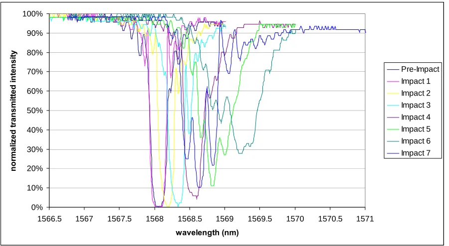
8 080705770030 Y 1567.17 1568.10 762.2

(48)

(49)

(50)

(a) (b)

(c) (d)

(51)

(52)

0% 10% 20% 30% 40% 50% 60% 70% 80% 90% 100%

1545.5 1545.7 1545.9 1546.1 1546.3 1546.5 1546.7 1546.9

wavelength (nm) n o rm al iz ed t ran sm it te d i n ten si ty Pre-Impact Impact 1 Impact 2 Impact 3 Impact 4 Impact 5 Impact 6 Impact 7 Impact 8 Impact 9 Impact 10 Impact 11 Impact 12

Figure 3.18. Normalized transmitted intensity after each impact for sensor #1 (080705770009). 0% 10% 20% 30% 40% 50% 60% 70% 80% 90% 100%

1566.5 1567 1567.5 1568 1568.5 1569 1569.5 1570 1570.5 1571

wavelength (nm) n o rm al iz ed t ran sm it ted in ten si ty Pre-Impact Impact 1 Impact 2 Impact 3 Impact 4 Impact 5 Impact 6 Impact 7

(53)

Table 3.6. Micro-strain after each strike for each sensor.

Strike FBG

Post-fab 1 2 3 4 5 6 7 8 9 10 11 12

1 195.7 246.5 269.8 212.3 189.1 204.8 197.2 171.8 172.5 166.5 182.2 195.5 207.8

2 473.8 514.3 537.1 544.5 490.7 491.1 469.8 482.3 470.9 553.5 553.8 550.4 557.5

3 696.7 646.0 712.1 733.0 750.8 754.2 770.1 755.2 752.5 762.2 757.0 738.5 756.2

4 644.7 652.1 655.3 802.3 817.3 801.7 809.3 801.2 803.1 787.3 891.7 801.4 800.4

5 85.4 107.9 239.6 162.3 169.9 151.7 138.5 153.6 139.7 150.4 123.5 148.2 192.7

6 295.8 280.0 401.2 392.3 415.2 421.2 422.7 414.7 417.7 401.4 369.3 364.9 348.6

7 341.5 420.2 582.0 593.7 624.0 596.1 606.4 605.3 613.4 614.3 609.1 605.6 603.6

8 762.2 705.9 788.3 889.3 1350.8 1555.5 1686.7 1196.9 ---- ---- ---- ---- ----

600 650 700 750 800

0 1 2 3 4 5 6 7 8 9 10 11 12

strike #

mic

ro

-s

tr

ain

(54)

CHAPTER FOUR: CONCLUSIONS AND FUTURE WORK

Conclusion

This study demonstrates that relatively high densities of embedded 250 μm diameter optical fibers may not have a negative effect on the host woven composite material during low velocity impact events. In this study, up to 6.3 optical fibers per centimeter were embedded within woven composite systems. While there did appear to be slight trends due to the presence of embedded fibers, there were no clear trends associated with the increase in embedded fiber densities. The fabrication method used within this study to embed optical fibers during fabrication of the composite specimens improved upon that previously applied, permitting greater fiber survivability and light transmission at higher cure pressures.

(55)

Suggestions for Future Work

Further optimization of the FBG sensor network for realistic applications needs to be investigated. For a predetermined impact location, it is evident that the sensor locations in this study were spaced too distant from the impact location to maximize damage information. However, increasing the density of the sensor network would increase the risk of deteriorating the impact resistance of the host material system. Therefore the optimum sensor density would need to be determined. To test the performance of any sensor network, impact events should also be applied at random locations rather than at a pre-determined single impact location to test the ability of the sensor network to not only measure damage but also the location of damage within the sensing area. Embedding sensors at varying depths within composites should be investigated for different applications and systems, such as thick and thin composites and differing impact energies.

More impact tests at various embedded fiber densities should be performed to determine more clearly the effect of the embedded fibers on the host material. There will be an optimal density which provides greatest sensing capability without causing mechanical degradation of the host material.

(56)

REFERENCES

Culshaw, B. "Basic Concepts of Optical Fiber Sensors," Optical Fiber Sensors: Principles and Components. Ed. John Dakin and Brian Culshaw. Boston: Artech House, 1988. 9-24.

Daniel, IM, and Ishai O, Engineering Mechanics of Composite Materials. 2nd ed. New York: Oxford UP, 2006.

Hill KO, Fujii Y, Johnson DC, . Kawasaki BS, "Photosensitivity in Optical Fiber

Waveguides: Application to Reflection Filter Fabrication," Applied Physics Letters

32,pp. 647-649, 1978.

Jensen DW, August JA, Pascual J, “Compressive Strength and Stiffness Reductions in Graphite/bismaleimide Laminates with Embedded Fibre-Optic Sensors”, ADPA/AIAA/SPIE Conference on Active Materials and Adaptive Structures, Alexandria, VA, Editor GJ Knowles, IOP, Bristol, p 129-134, 1991.

Jenson DW, Pascual J, “Degradation of Graphite/bismaleimide Laminates with Multiple Embedded Fiber Optic Sensors,” Proc. SPIE, 1370, p. 228, 1990.

Kersey, AD, Optical Fiber Sensors: Applications, Analysis, and Future Trends. Ed. John Dakin and Brian Culshaw. Vol. 4. Boston: Artech House,. pp. 374-375, 1997 Kuang KSC, Kenny R, Whelan MP, Cantwell WJ, Chalker PR, “Residual strain

measurement and impact response of optical fibre Bragg grating sensors in fibre metal laminates,” Smart Materials and Structures, 10, pp. 338-346, 2001.

LeBlanc M, Measures R, “Impact Damage Assessment in Composite Materials with Embedded Fibre-Optic Sensors,” Composites Engineering, 2, pp. 573-596, 1992.

Mall S, Dosedel SB, Holl MW, “Performance of Graphite-Epoxy Composites with

Embedded Optical Fibres under Compression,” Smart Materials and Structures, 5,

pp. 209-215, 1996.

Pearson J, “An Integrated Global-Local System for the Detection and Monitoring of Damage Progression in Heterogeneous Materials”, MS Thesis, North Carolina State

University, 2005.

Pearson J, Zikry MA, Prabhugoud M, and Peters K, “Global-Local Assessment of Low-Velocity Impact Damage in Woven Composites,” to appear in Journal of Composite Materials, 2007.

(57)

(58)

(a)

(b)

(59)

(a)

(b)

(60)

(61)

C2 - Contact Force 0 5000 10000 15000 20000 25000 30000

1 2 3 4 5 6 7 8 9 10 11 12 13 14 15 16 17 18 19 20 21 22 23 24 25 26 27 28 29 30 31 32 33 34 35

Strike # C ontact F o rc e N 12000 2 m/s Strikes Raw 1st Average 2nd Average 0 2000 4000 6000 8000 10000

Figure A.4. Contact force for specimen C2.

0.0 2.0 4.0 6.0 8.0 10.0 12.0

1 2 3 4 5 6 7 8 9 10 11 12 13 14 15 16 17 18 19 20 21 22 23 24 25 26 27 28 29 30 31 32 33 34 35

Strike # D issi pa te d Ener g y ( J )

(62)

C3 - Contact Force 0 5000 10000 15000 20000 25000 30000

1 2 3 4 5 6 7 8 9 10 11 12 13 14 15 16 17 18 19 20 21 22 23 24 25 26 27 28 29 30 31 32 33 34 35 36 Strike # C ont ac t F or c e N 10000 2 m/s Strikes Raw 1st Average 2nd Average 0 1000 2000 3000 4000 5000 6000 7000 8000 9000

0.0 2.0 4.0 6.0 8.0 10.0 12.0

1 2 3 4 5 6 7 8 9 10 11 12 13 14 15 16 17 18 19 20 21 22 23 24 25 26 27 28 29 30 31 32 33 34 35 36 Strike # D issi pat e d Ener gy ( J )

(63)

C4 - Contact Force 0 5000 10000 15000 20000 25000 30000

1 2 3 4 5 6 7 8 9 10 11 12 13 14 15 16 17 18 19 20 21

Strike # C on tac t F or c e N 0 2000 4000 6000 8000 10000 12000 2 m/s Strikes Raw 1st Average 2nd Average

0.0 2.0 4.0 6.0 8.0 10.0 12.0

1 2 3 4 5 6 7 8 9 10 11 12 13 14 15 16 17 18 19 20 21

Strike # D issi pat e d Ener gy ( J )

(64)

C5 - Contact Force 0 5000 10000 15000 20000 25000 30000 35000 40000

1 2 3 4 5 6 7 8 9 10 11 12 13 14 15 16 17 18 19 20 21 22 23

Strike # C o nt a c t F o rc e N 0 2000 4000 6000 8000 10000 12000 14000 16000 2 m/s Strike raw 1st average 2nd average

0.0 2.0 4.0 6.0 8.0 10.0 12.0

1 2 3 4 5 6 7 8 9 10 11 12 13 14 15 16 17 18 19 20 21 22 23

Strike # D iss ip at ed E n er gy (J)

(65)

C6 - Contact Force 0 5000 10000 15000 20000 25000 30000 35000 40000 45000

1 3 5 7 9 ₁₁ ₁₃ ₁₅ ₁₇ ₁₉ ₂₁ ₂₃ ₂₅ ₂₇ ₂₉ ₃₁ ₃₃ ₃₅ ₃₇

Strike # Co ntact Force N 0 2000 4000 6000 8000 10000 12000 14000 16000 18000 20000 2 m/s Strikes Raw

1st Average 2nd Average

0.0 2.0 4.0 6.0 8.0 10.0 12.0

(66)

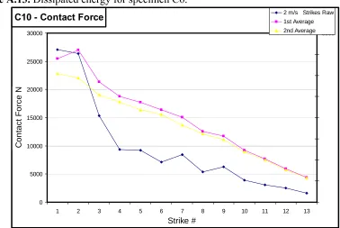
Figure A.13. Dissipated energy for specimen C6. C10 - Contact Force

0 5000 10000 15000 20000 25000 30000

1 2 3 4 5 6 7 8 9 10 11 12 13

Strike # C o nt act F o rc e N 0 1000 2000 3000 4000 5000 6000 7000 8000 2 m/s Strikes Raw 1st Average 2nd Average

Figure A.14. Contact force per strike for specimen C10.

0.0 2.0 4.0 6.0 8.0 10.0 12.0

1 2 3 4 5 6 7 8 9 10 11 12 13

Strike # D is ipat ed E ner gy ( J )

(67)

C11 - Contact Force 0 5000 10000 15000 20000 25000 30000

1 3 5 7 9 ₁₁ ₁₃ ₁₅ ₁₇ ₁₉ ₂₁ ₂₃ ₂₅ ₂₇ ₂₉ ₃₁ ₃₃ ₃₅ ₃₇ ₃₉ ₄₁ ₄₃ ₄₅ ₄₇ ₄₉

Strike # C on tac t F or c e N 0 1000 2000 3000 4000 5000 6000 7000 8000 9000 2 m/s Strikes Raw 1st Average 2nd Average

0.0 2.0 4.0 6.0 8.0 10.0 12.0

1 3 5 7 9 ₁₁ ₁₃ ₁₅ ₁₇ ₁₉ ₂₁ ₂₃ ₂₅ ₂₇ ₂₉ ₃₁ ₃₃ ₃₅ ₃₇ ₃₉ ₄₁ ₄₃ ₄₅ ₄₇ ₄₉

(68)

C12 - Contact Force 0 5000 10000 15000 20000 25000 30000

1 2 3 4 5 6 7 8 9 10 11 12 13 14 15 16

Strike # C ont ac t F o rc e N 8000 2 m/s Strikes Raw 1st Average 2nd Average 0 1000 2000 3000 4000 5000 6000 7000

0.0 2.0 4.0 6.0 8.0 10.0 12.0

1 2 3 4 5 6 7 8 9 10 11 12 13 14 15 16

Strike # Di si pat ed E ner gy ( J )

(69)

C14 - Contact Force 0 5000 10000 15000 20000 25000 30000

1 2 3 4 5 6 7 8 9 10 11 12 13 14 15 16 17 18 19 20 21 22 23 24 25 26 27 28 29 30 31

Strike # C ontac t For c e N 12000 2 m/s Strikes Raw 1st Average 2nd Average 0 2000 4000 6000 8000 10000

0.0 2.0 4.0 6.0 8.0 10.0 12.0 14.0

1 2 3 4 5 6 7 8 9 10 11 12 13 14 15 16 17 18 19 20 21 22 23 24 25 26 27 28 29 30 31

Strike # D is ipat ed Ene rgy ( J)

(70)

0% 20% 40% 60% 80% 100%

1544 1545 1546 1547 1548

wavelength (nm) P er cen t tr an sm is si o n Pre-fab Post-fab

Figure A.22. Spectral response of FBG #1 (080705770009).

0% 20% 40% 60% 80% 100%

1547 1548 1549 1550 1551

wavelength (nm) P er ce n t t ran sm issi o n Pre-fab Post-fab

(71)

0% 20% 40% 60% 80% 100%

1550 1550.5 1551 1551.5 1552 1552.5 1553 1553.5 1554

wavelength (nm) P er cen t tr an sm is si o n Pre-Fab Post-Fab

0% 20% 40% 60% 80% 100%

1553 1553.5 1554 1554.5 1555 1555.5 1556 1556.5 1557

wavelength (nm) P er ce n t t ran sm issi o n Pre-Fab Post-Pab

(72)

0% 20% 40% 60% 80% 100%

1556 1557 1558 1559 1560

0% 20% 40% 60% 80% 100%

1559 1560 1561 1562 1563

wavelength (nm) P er ce n t t ran sm issi o n Pre-Fab Post-Fab

(73)

0% 20% 40% 60% 80% 100%

1562 1563 1564 1565 1566

0% 20% 40% 60% 80% 100%

1565 1566 1567 1568 1569 1570 1571

wavelength (nm) P er ce n t t ran sm issi o n Pre-Fab Post-Fab

(74)

0% 10% 20% 30% 40% 50% 60% 70% 80% 90% 100%

1548 1548.5 1549 1549.5 1550 1550.5 1551

wavelength (nm) n o rm aliz ed t ra n sm it te d in te n si ty Pre-Impact Impact 1 Impact 2 Impact 3 Impact 4 Impact 5 Impact 6 Impact 7 Impact 8 Impact 9 Impact 10 Impact 11 Impact 12

Figure A.30. Normalized transmitted intensity per strike for sensor #2 (080705770012).

0% 10% 20% 30% 40% 50% 60% 70% 80% 90% 100%

1551.5 1552 1552.5 1553 1553.5 1554

wavelength (nm) n o rma liz ed t ra n sm it te d in te n sit y Pre-impact Impact 1 Impact 2 Impact 3 Impact 4 Impact 5 Impact 6 Impact 7 Impact 8 Impact 9 Impact 10 Impact 11 Impact 12

(75)

0% 10% 20% 30% 40% 50% 60% 70% 80% 90% 100%

1554.5 1555 1555.5 1556 1556.5 1557

wavelength (nm) n o rm alize d t ra n sm it te d in te n si ty Pre-Impact Impact 1 Impact 2 Impact 3 Impact 4 Impact 5 Impact 6 Impact 7 Impact 8 Impact 9 Impact 10 Impact 11 Impact 12

0% 10% 20% 30% 40% 50% 60% 70% 80% 90% 100%

1557.2 1557.4 1557.6 1557.8 1558 1558.2 1558.4 1558.6 1558.8 1559

wavelength (nm) n o rma lize d t ra n smit te d in te n sit y Pre-Impact Impact 1 Impact 2 Impact 3 Impact 4 Impact 5 Impact 6 Impact 7 Impact 8 Impact 9 Impact 10 Impact 11 Impact 12

(76)

0% 10% 20% 30% 40% 50% 60% 70% 80% 90% 100%

1560 1560.5 1561 1561.5 1562 1562.5 1563

wavelength (nm) n o rm alize d t ra n sm it te d in te n si ty Pre-Impact Impact 1 Impact 2 Impact 3 Impact 4 Impact 5 Impact 6 Impact 7 Impact 8 Impact 9 Impact 10 Impact 11 Impact 12

0% 10% 20% 30% 40% 50% 60% 70% 80% 90% 100%

1563.5 1563.7 1563.9 1564.1 1564.3 1564.5 1564.7 1564.9 1565.1 1565.3 1565.5

wavelength (nm) n o rm ali ze d t ra n sm it te d in te n sit y Pre-Impact Impact 1 Impact 2 Impact 3 Impact 4 Impact 5 Impact 6 Impact 7 Impact 8 Impact 9 Impact 10 Impact 11 Impact 12

(77)