A Quantitative Trait Locus Mixture Model That Avoids
Spurious LOD Score Peaks
Bjarke Feenstra
1and Ib M. Skovgaard
Department of Natural Sciences, Royal Veterinary and Agricultural University, DK-1871 Frederiksberg C, Denmark Manuscript received December 5, 2003
Accepted for publication February 13, 2004
ABSTRACT
In standard interval mapping of quantitative trait loci (QTL), the QTL effect is described by a normal mixture model. At any given location in the genome, the evidence of a putative QTL is measured by the likelihood ratio of the mixture model compared to a single normal distribution (the LOD score). This approach can occasionally produce spurious LOD score peaks in regions of low genotype information (e.g., widely spaced markers), especially if the phenotype distribution deviates markedly from a normal distribution. Such peaks are not indicative of a QTL effect; rather, they are caused by the fact that a mixture of normals always produces a better fit than a single normal distribution. In this study, a mixture model for QTL mapping that avoids the problems of such spurious LOD score peaks is presented.
F
OR more than a decade, interval mapping (Lander than the single-component model, even in a model with-andBotstein1989) has been the most commonly out any genetic (marker) information and even if there used method for quantitative trait locus (QTL) mapping is no real QTL.in experimental crosses. Often, interval mapping is used As an example, consider the following preliminary to identify regions of interest in the genome, which data set from an ongoing study of yellow rust (Puccinia
are then analyzed with more refined methods such as striiformis) resistance in wheat (Triticum aestivum): 55 composite interval mapping (Zeng1993, 1994) or multi- doubled haploid lines (DHLs; see, for example,Lynch ple interval mapping (Kao et al.1999). In cases where andWalsh1998) were scored for rust resistance using interval mapping suggests the existence of a QTL in a a 0–9 scale in which 0 is no rust and 9 is total infection. region that is sparsely covered with markers, it may be The phenotypes were taken to be the scores divided by decided to develop more markers in this region to map 10 and arc sine square root transformed, a transforma-the putative QTL more accurately. There may, however, tion often used for observations on a finite interval. The be situations where interval mapping produces strong DHLs were genotyped for a suite of microsatellite markers evidence for a QTL, when in fact there is none. If, for and interval mapping was performed (Figure 1). instance, the residual environmental variation does not As can be seen from Figure 1, there were three large follow a normal distribution, interval mapping can re- LOD score peaks that all occurred in regions where the sult in spurious LOD score peaks in regions of low geno- markers were very far apart (80–100 cM). Also, it was type information (e.g., widely spaced markers or much noted that when all genotype information was disre-missing marker data;Broman2003). garded and a mixture of two normal distributions was In standard interval mapping the distribution of the fitted to the phenotypic data, this resulted in a LOD phenotype is modeled as a mixture of two (or more) score of 9.83 compared to a single normal distribution. components corresponding to the two (or more) different The fact that the three LOD score peaks were of the genotypes at the putative QTL (Landerand Botstein same order of magnitude as the LOD score based on 1989). When a specific basic distribution like the normal no genotype information and that the peaks occurred in is used for each component this approach has the side regions of little genotype information strongly suggests effect that even without genetic (marker) information that these peaks are artifacts.
the distribution is a mixture of two or more normals In the wheat data set, visual inspection of the pheno-when a QTL is included in the model, while under
type distribution (Figure 2) hints that in areas of little the null hypothesis of no QTL there is only a single
genotype information a mixture of two normal distribu-component. If the basic distribution is not normal the
tions could produce a better fit than a single normal model including a QTL may fit to data much better
distribution, and hence that spurious LOD score peaks could occur.
In other cases, however, it may be less clear whether
1Corresponding author:Department of Natural Sciences, Royal
Veteri-a LOD score peVeteri-ak is Veteri-an Veteri-artifVeteri-act or not. We present nary and Agricultural University, Thorvaldsensvej 40, DK-1871
Freder-iksberg C, Denmark. E-mail: [email protected] a new model (Equation 1) that is a mixture of two
Figure1.—Spurious LOD score peaks pro-duced by standard interval mapping of data from 55 DHLs in wheat. The corresponding LOD score curve from the two-component mixture model (1) is included for compari-son. The segments 1A, 2B, . . . , 7D represent different chromosomes.
components whether a QTL is present or not and there- where f(y; , ) is the density function for a normal distribution with meanand standard deviation. The fore avoids the problems of such spurious LOD score
peaks (see Figure 1). indexjmay be thought of as the genotype at the putative QTL. The number pij is the conditional probability, given the marker data and the QTL position, that indi-METHODS
vidualihas genotypej. The distribution of the pheno-type of individuals with genopheno-typej is now (unconven-For simplicity, we consider a sample ofnindividuals
from a backcross (BC) population (see, for example, tionally) modeled as a mixture of the two normal LynchandWalsh1998), but the results extend easily to components with weights j and 1⫺ j, respectively. other kinds of crosses. Letyiandmidenote the quantitative Under normal assumptions we would like to see the phenotype and the multipoint marker data, respectively, estimates of these weights at a QTL position close to for individuali. zero or one, indicating that a given genotype essentially
To avoid the problem of spurious LOD score peaks results in a single-component normal distribution. we make sure that the model satisfies the following re- The likelihood function may be rewritten as quirements: the distribution has the same number of
L()⫽
兿
i
(cif(yi;1,)⫹ (1⫺ci)f(yi;2,)), (2) components whether a QTL is present or not; without
genetic information the model with and without a QTL
where ci ⫽兺jpijjis the weight of the first component is the same; and the model contains our original genetic
in the two-component mixture distribution for individ-model as a special case.
uali. More concretely, the likelihood function of the
pa-Now, the null hypothesis of no QTL effect is rameter vector ⫽(1,2,,1,2) is given by
H0:j⫽ , for allj,
L()⫽
兿
i
兺
jpij(jf(yi;1,)⫹(1⫺ j)f(yi;2,)),
(1) implying that the distribution does not depend on the genotype of the putative QTL. The corresponding likeli-hood function is
L()⫽
兿
i
(f(yi;1,)⫹(1⫺ )f(yi;2,)), (3)
which, again, is a mixture of two normal distributions as required. In this case, however, the mixture coeffi-cients do not depend on the QTL genotypes. Thus, the likelihood under H0is calculated just once.
Under the full model, we obtain maximum-likelihood estimates of the parameters with a form of the expecta-tion-maximization (EM) algorithm (Dempster et al.
1977). In the following, letzibe an unobserved variable indicating whether the observation yi comes from the first component (zi⫽1) or from the second component (zi ⫽ 2) of the mixture. Letqi be another unobserved variable indicating the true genotype at the putative
Figure 2.—Histogram of transformed disease resistance
QTL for individual i(i.e.,qi⫽ 1 orqi ⫽2). Assume at scores of 55 DHLs in wheat. Approximately 30% of the DHLs
the observed phenotypes. To do so, we calculate three ⫽ ˆ f(yi;ˆ1 ,ˆ )
ˆ(s)f(yi;ˆ( s) 1 ,ˆ(
s))⫹(1⫺ ˆ(s) )f(yi;ˆ(
s) 2 ,ˆ(
s))(8) different weights for each individual. First, for each of
the two components in the mixture distribution, and
w(s⫹1)
i,1 ⫽ Pr(zi ⫽1|yi,mi,ˆ(s)) w(i,2s⫹1)⫽1⫺w(i,1s⫹1).
In the M-step, we obtain updated parameter estimates
⫽ cˆ(is)f(yi;ˆ( s) 1 ,ˆ(
s))
cˆ(is)f(yi;ˆ( s)
1 ,ˆ(s))⫹(1 ⫺cˆ (s)
i )f(yi;ˆ( s)
2 ,ˆ(s)) of1,2, andusing Equations 4 and 5 and estimate
by the following equation: and
ˆ(s⫹1)⫽
兺
iw( s⫹1) i,1n . (9)
w(i,2s⫹1)⫽1⫺w (s⫹1) i,1 .
Second, for each of the two possible QTL genotypes,
We initiate the EM algorithm by taking w(0) i,l ⫽0.5, which, however, causesˆ(0)1 andˆ
(0)
2 to be equal andˆ(0)
u(s⫹1)
i,1 ⫽Pr(qi⫽1|yi,mi,ˆ(s))
to be 0.5. In that case, as is seen from Equation 8, the weights and estimates are not changed by the iterations.
⫽pi1ˆ1(s)f(yi;ˆ (s) 1 ,ˆ(
s))⫹ p
i1(1 ⫺ ˆ (s) 1 )f(yi;ˆ
(s) 2 ,ˆ(
s))
cˆ(is)f(yi;ˆ( s) 1 ,ˆ(
s))⫹(1 ⫺cˆ(s) i )f (yi;ˆ(
s) 2 ,ˆ(
s))
This is a consequence of the symmetry of the model in the two components; in fact1⫽ 2⫽yis a stationary and
point on the likelihood surface. Thus, to prevent the
u(i,2s⫹1)⫽1⫺u (s⫹1)
i,1 . algorithm from getting stuck, we offset the initial values slightly in opposite directions. We iterate until Third, for the combination of mixture component and
the estimates converge. QTL genotype,
v(s⫹1)
i ⫽Pr(ziqi⫽1|yi,mi,ˆ(s))
SIMULATIONS
⫽ pi1ˆ1(s)f(yi;ˆ( s) 1 ,ˆ(
s))
cˆ(is)f(yi;ˆ( s) 1 ,ˆ(
s))⫹ (1⫺cˆ(s) i )f (yi;ˆ(
s) 2 ,ˆ(
s)). To illustrate the properties of the two-component mixture model and to compare its performance with standard interval mapping, we performed a small simu-In the M-step, updated estimates of1,2,,1, and
lation study. We assessed the occurrence of spurious
2are given by
LOD score peaks by simulating 80 BC individuals under a null model of no QTL. We simulated 12 chromosomes,
ˆ(ls⫹1)⫽
兺
iw(s⫹1) i,l yi
兺
iw( s⫹1) i,l(4)
each 120 cM long and each with four to nine randomly distributed markers. A random 10% of the marker geno-type data was missing. Phenogeno-types were simulated from
ˆ(s⫹1)⫽
冪
1n
兺
i兺
l (yi⫺ ˆ(s⫹1) l )2w
(s⫹1)
i,l (5)
a threshold model; first a random number was drawn from a standard normal distribution and then it was rounded upward to the nearest of the following
thresh-ˆ(1s⫹1)⫽
兺
iv(s⫹1) i
兺
iu( s⫹1) i,l(6)
olds: 0, 0.5, 1, 1.5, 2, 2.5, 3, 3.5, 4, 4.5, and 5.0. The phenotype was taken to be the threshold value in
ques-ˆ(2s⫹1)⫽
兺
i(w(s⫹1) i,1 ⫺v
(s⫹1) i )
兺
iu( s⫹1) i,2Figure 3.—Maximum LOD score as a function of the length of the interval where the maximum oc-curred for 2000 simulated data sets.
LOD scores in intervals ⬎80 cM was twice that of the lower power compared to that of standard interval map-two-component model (108vs.50). ping. To translate the power loss to the relative number It might be expected that the price of extending the of observations we used the approximate relationship model, as we do in the two-component mixture model,
(Q)⬇1⫺ ⌽(z␣/2⫺Q
√
nC)⫹ ⌽(⫺z␣/2⫺Q√
nC) , is a loss of power. To compare power and precision ofthe two-component model with the standard interval
where is the power function,Q is the QTL effect,C
mapping model, we simulated 200 BC individuals under
is a constant, nis the number of individuals, ⌽is the a single-QTL model. We simulated five chromosomes,
standard normal distribution function, andz␣/2denotes each 100 cM long and each with 11 randomly distributed
the upper␣/2 quantile of the standard normal distribu-markers and a QTL at position 60 cM on chromosome
tion. On the basis of this relationship, the power loss 1. We considered six different values of the additive
of the two-component model corresponded to ⵑ12% effect of the QTL: 0 (null model), 0.12, 0.20, 0.26, 0.32,
fewer observations in the standard interval mapping and 0.38. The trait value of an individual was
deter-model. The approximation holds in general for two-mined by a random (environmental) variable drawn
sided tests of a parameter in a well-behaved statistical from a standard normal distribution plus the QTL effect
model (see van der Vaart 1998, Chap. 14), but in (QTL genotype 2)orminus the QTL effect (QTL
geno-the present setting we use it only empirically without type 1). We performed 5000 simulations and analyzed
claiming any theoretical justification. We also estimated all six QTL effects with both standard interval mapping
the precision in locating the QTL by means of the root-and the two-component mixture model. We obtained
mean-square (RMS) error of the estimated QTL posi-genome-wide LOD thresholds from the data with no
tion (Figure 5B). The two methods had very similar QTL effect, as the 95th percentiles of the maximum
precision of QTL localization, although interval map-LOD score. The map-LOD thresholds for standard interval
ping had a marginally greater precision (smaller RMS mapping and the two-component mixture model were
error) compared to that of the two-component model. 2.26 and 2.48, respectively. Figure 4 shows a simulation
The additive QTL effect was estimated in somewhat example. LOD scores were calculated and plotted at
different ways under the two models. Since in the simula-every 2 cM. It can be seen from the figure that in a
tions the QTL genotype indexed byj⫽2 corresponded data set not leading to spurious LOD score peaks, the
to a positive additive effect, the QTL effect under standard evidence obtained by standard interval mapping and
interval mapping was estimated asaˆIM⫽0.5 · (ˆ2⫺ ˆ1). the two-component model may be very similar.
In the case of the two-component model, the QTL effect The power of the two methods was estimated as the
was estimated asaˆ2C⫽0.5 · (ˆ2ˆ1⫹(1⫺ ˆ2)ˆ2⫺ ˆ1ˆ1⫺ proportion of the simulation replicates for which the
(1⫺ ˆ1)ˆ2). In each case, the QTL effect was estimated maximum LOD score exceeded the corresponding
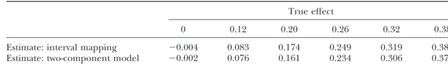
at the position of the maximum LOD score. True and LOD threshold. As can be seen in Figure 5A, the
Figure4.—A simulation example of QTL mapping on a population of 200 BC individuals. The QTL position is indicated by the triangle on thex-axis. The additive effect of the QTL increases in six steps from 0 (bottom solid curve) to 0.38 (top dashed curve). Standard interval mapping (left) and the two-component mixture model (right) applied to the same data set are compared. Genome-wide LOD thresholds are indicated by the dotted horizontal lines.
produced estimates slightly lower than the true values, null hypothesis of no QTL there is only a single compo-nent. Now, if the phenotype distribution is not normal, since sometimes aˆIM andaˆ2C were negative by chance.
Note, however, that the estimates come very close to the two- (or more) component model may fit to data much better than the single-component model, even in the true value as the QTL effect increases.
a model without any genetic information and even if there is no real QTL. Thus, in cases where the pheno-DISCUSSION
type distribution deviates from a normal distribution, false-positive results may be obtained in regions of low We have demonstrated that the commonly used
stan-dard interval mapping method may occasionally result genotype information (e.g., widely spaced markers, low degree of polymorphism, or much missing marker in spurious LOD score peaks. In interval mapping the
distribution is a mixture of two (or more) components data). The problem was seen in an application (Figure 1). Close inspection of Figure 1 reveals that the LOD when a QTL is included in the model while under the
TABLE 1
True and estimated QTL effects from 5000 simulation replicates
True effect
0 0.12 0.20 0.26 0.32 0.38
Estimate: interval mapping ⫺0.004 0.083 0.174 0.249 0.319 0.380 Estimate: two-component model ⫺0.002 0.076 0.161 0.234 0.306 0.371
Standard error of the means ranged from 0.0012 to 0.0025.
score curve jumps rather abruptly at the peaks. This is distribution (a large portion of the individuals share a common phenotype value) this may be modeled by a due partly to numerical difficulties in finding the global
maximum of the likelihood function in the vicinity of two-part parametric model (Broman 2003). However, the two-part model may also produce spurious LOD the peaks. Thus, improved algorithms would widen and
smoothen the peaks, but would not diminish their size. score peaks since one of its two parts is a mixture of two (or more) normal distributions when a QTL is in-We have presented a mixture model for QTL
map-ping that avoids this artifact. Our model is a mixture of cluded in the model, but only a single normal distribu-tion under the null hypothesis. Thus, while the part two normal distributions (BC or DHL data) whether or
not a QTL is included in the model; the QTL affects corresponding to the common phenotype alleviates the problem, it may still occur if the remaining phenotype the mixing probabilities instead of the number of
com-ponents. Our simulation results indicate that the two- values deviate from a single normal distribution. One might also take a nonparametric approach to mapping component mixture model has only a minor loss of
power and comparable precision to standard interval QTL in the case of nonnormal phenotype distributions (KruglyakandLander1995;Broman2003). Although mapping in locating QTL over a range of QTL effects.
The results of analysis with the two-component mix- generally a powerful alternative, nonparametric meth-ods provide only a test for the presence of a QTL, ture model must be interpreted with some care. In the
case of a backcross population, we would like the abso- whereas parametric methods also estimate the pheno-typic effect of the QTL.
lute difference between1and2 of Equation 1 to be
close to 1 at a QTL position. This would indicate that With the advent of extremely dense marker maps in a large number of species, it might be argued that the QTL genotypes from the parental lines each result
in a single (different) normal distribution. In our simu- researchers need not be concerned about getting spuri-ous LOD score peaks from interval mapping. However, lations, increasing the additive QTL effect from 0.12 to
0.38 caused the mean of |ˆ1 ⫺ ˆ2| at the true QTL in many agriculturally important species only few mark-ers have been developed, and even in species with many location for data sets with LOD⬎2.48 at that position
to increase from 0.56 to 0.73 (data not shown). While markers available, initial analyses may be undertaken with few markers to identify important regions of the these numbers are not that close to 1, it should be
kept in mind that the residual variance used in the genome. Moreover, the marker map may be dense and yet the genetic data may have poor information content, simulations was quite large at 1 compared to the additive
QTL effects of 0.12–0.38. Also, it was noted that for a if, for example, the markers are dominant or if the proportion of missing data at certain marker loci is high. given QTL effect, the estimated difference between1
and 2 increased with increasing LOD score. Still, it Also, it should be noted that the type of cross influences the risk of spurious LOD peaks from interval mapping. appears that the QTL effect needs to be larger
com-pared to the residual variance for the mixing parameters In the case of F2intercross populations (see, for exam-ple, LynchandWalsh1998), the phenotype is
mod-1and2to be better estimated.
Several different numerical optimizations may be con- eled as a mixture of three components. In regions of low genotype information, the three-component mix-sidered; the EM algorithm is often found to be
some-what slow but fairly robust and easy to program. As with ture distribution produces a better fit than a two-compo-nent mixture distribution. Thus, spurious LOD peaks other methods, there is no guarantee that it will find
the global maximum rather than a local maximum, or are expected to be more of a problem in F2intercrosses compared to, for instance, backcrosses or DHLs. For F2 even get stuck in a local minimum, but in our examples
it seemed to work well, as judged from the LOD scores intercrosses, our two-component model may be ex-tended to three components in a straightforward man-and other results obtained.
Other methods for QTL mapping have been devel- ner. However, problems with false or no convergence generally increase with the number of components in oped for cases where the phenotype distribution is
a spike in the phenotype distribution. Genetics163:1169–1175. here. For example, it is well known that analyzing a
Broman, K. W., H. Wu, S´. SenandG. A. Churchill, 2003 R/qtl: chromosome holding two linked QTL with a single-QTL
QTL mapping in experimental crosses. Bioinformatics19:889– model may result in a so-called “ghost” QTL (Knott 890.
Dempster, A. P., N. M. LairdandD. B. Rubin, 1977 Maximum andHaley1992;Martı´nezandCurnow1992). While
likelihood from incomplete data via the EM algorithm. J. R. Stat. avoiding spurious LOD score peaks from low genotype
Soc. B39:1–38.
information, the two-component model is not guaran- Ihaka, R., andR. Gentleman, 1996 R: a language for data analysis and graphics. J. Comp. Graph. Stat.5:299–314.
teed to avoid all spurious LOD score peaks.
Kao, C.-H., Z-B. ZengandR. D. Teasdale, 1999 Multiple interval In conclusion, the mixture model presented here may mapping for quantitative trait loci. Genetics152:1203–1216. be preferred in situations of large intermarker distances, Knott, S. A., andC. S. Haley, 1992 Aspects of maximum likelihood
methods for the mapping of quantitative trait loci in line crosses. dominant markers, low sample sizes, low degree of
poly-Genet. Res.60:139–151.
morphism in markers, or much missing marker informa- Kruglyak, L., andE. S. Lander, 1995 A nonparametric approach tion. Spurious LOD score peaks arising from standard for mapping quantitative trait loci. Genetics139:1421–1428.
Lander, E. S., andD. Botstein, 1989 Mapping Mendelian factors interval mapping may be identified if they cannot be
underlying quantitative traits using RFLP linkage maps. Genetics reproduced by the mixture model presented here. 121:185–199.
The simulations and interval mapping analyses in this Lynch, M., andB. Walsh, 1998 Genetics and Analysis of Quantitative Traits. Sinauer, Sunderland, MA.
article were done with R/qtl (Bromanet al.2003), an
Martı´nez, O., andR. N. Curnow, 1992 Estimating the locations add-on package for the general statistical software,R and the sizes of the effects of quantitative trait loci using flanking
markers. Theor. Appl. Genet.85:480–488. (Ihaka and Gentleman 1996). The simulation study
Rossini, A., L. TierneyandN. Li, 2003 Simple parallel statistical benefited from parallelization using the R-package
computing in R. University of Washington Biostatistics Working SNOW (Rossiniet al.2003). The two-component model Paper Series 193, University of Washington, Seattle.
van der Vaart, A. W., 1998 Asymptotic Statistics. Cambridge Univer-was implemented with a couple of new functions within
sity Press, Cambridge, UK. the framework of R/qtl; the source code can be
ob-Zeng, Z-B., 1993 Theoretical basis of separation of multiple linked tained by contacting the corresponding author. gene effects on mapping quantitative trait loci. Proc. Natl. Acad.
Sci. USA90:10972–10976. We are grateful to two anonymous reviewers for their constructive
Zeng, Z-B., 1994 Precision mapping of quantitative trait loci. Genet-comments, which led to improvements of the presentation and of the ics136:1457–1468.
numerical optimization method. We thank Merethe J. Christiansen at