An Efficient Mode Reduction Technique for Modeling
of Waveguide Gratings
Lijun Yuan1 and Yu Mao Wu2, *
Abstract—In this paper, an efficient mode reduction technique for eigenmode expansion method is developed to analyze 2–D waveguide grating structures which are a special class of piecewise uniform waveguides. To take advantage of the periodicity property of the structure, the eigenmode expansion method (EEM) is used with the scattering matrix method and a recursive-doubling procedure. In this situation, our proposed mode reduction technique achieves a significant speedup for gratings with large number of periods. Comprehensive numerical examples on the waveguide gratings are studied to validate the efficiency of our proposed mode reduction technique.
1. INTRODUCTION
Waveguide grating structures that are piecewise uniform and periodic in the longitudinal direction are widely used in many modern optical devices. Numerical simulations of the wavefields are essential in the design and analysis of these structures. Existing methods for analyzing such structures with multiple longitudinal discontinuities include various eigenmode expansion methods (EEM) [1–7], the bidirectional beam propagation method (BiBPM) [8–12], the finite difference time domain (FDTD) method [13] and the quation integral method [14, 15]. Efficient numerical techniques are in great need for modeling the wavefields of the considered structures.
In various EEM, the wave field in each longitudinally uniform segment is expanded in terms of the eigenmodes of the transverse operator. For an open waveguide, the transverse direction has to be truncated into finite interval by adopting absorbing boundary conditions, such as the perfectly matched layers (PMLs) [16, 17]. After that, the eigenmodes can be calculated semi-analytically by solving a nonlinear equation, if the refractive index profile in each segment is piecewise constant in the transverse direction. On invoking the PMLs, the propagation constants of eigenmodes may be complex. Hence, it is not a simple task to compute all solutions from this nonlinear equation in the complex domain. In this situation, eigenmodes can be efficiently calculated by numerical methods such as the finite element method [1], the finite difference method [4], and Fourier series [6, 7]. If transverse direction is discretized with N grid points, eigenmodes of each segment can be computed by O(N3) operations. Since the waveguide grating is periodic, the eigenvalue problem only needs to be solved in two segments. Meanwhile, EEM can be implemented in serval different ways. One of the widely used and robust method is the scattering matrix method [6, 18]. For a 2D waveguide grating withmperiods, scattering matrix method needs O(mN3) operations. By adopting the recursive-doubling procedures, the number of operations can be reduced toO(N3log2m).
The BiBPMs rely on the rational approximation of a square root operator and its exponential. For deeply etched waveguides with large index-contrast, BiBPMs are very difficult to model the radiation
Received 3 October 2014, Accepted 13 November 2014, Scheduled 21 November 2014 * Corresponding author: Yu Mao Wu ([email protected]).
and evanescent modes. FDTD [13] is a widely used method in the simulation of optical structures. But it requires a small grid size to resolve large index-contrast and a small time step to ensure numerical stability. Integral equation method [14, 15] offers an efficient way to analyze bandgaps of photonic crystals and reflectance of waveguides. Furthermore, on invoking the integral equation method, only the surface needs to discretize and avoids the discretization of the whole computation domain, and therefore significantly reduce the number of unknowns [14]. Meanwhile, integral equation method also can efficiently simulate very complicate geometries. In [15], an integral equation method was extensively studied, and then adopted to analyze the optical response from PEC waveguide composed of two periodic and one-dimensional rough surfaces.
In this paper, we develop a mode reduction technique for the analysis of 2D waveguide grating with large number of periods. After the process that the scattering matrix of one period is calculated using the full set of eigenmodes, our approach can significantly reduce the number of modes used in the construction of the scattering matrix of the whole structure. By using a recursive doubling procedure, our approach can reduce the total number of operations toO(N3) +O(N∗3log2m), whereN∗ (N∗ < N) is the number of retained modes. For structures with largem, a significant speedup could be achieved. The error induced by our mode reduction technique is small even the number of retained eigenmodes
N∗ is less than one third of N. In the future, it is possible to extend our approach to analyze 3D
waveguides and 2D slab photonic structures.
2. PROBLEM FORMULATION
Let{x, y, z} be a Cartesian coordinate system, we consider the structure and the electromagnetic field are both independent of z. Then, the z–components of the time harmonic field satisfy the following Helmholtz equation
ρ ∂ ∂x
1
ρ ∂u ∂x
+ρ ∂ ∂y
1
ρ ∂u ∂y
+k02εμ u= 0, (1)
where k0 is the free space wavenumber, ε the relative permittivity, and μ the relative permeability. u = Ez and ρ = μ correspond to the transverse electric (TE) polarization. u = Hz and ρ = ε
correspond to the transverse magnetic (TM) polarization.
A piecewise uniform waveguide with the main propagation direction in x is a structure with discontinuity points x1 < x2 < . . . < xm, such that ε and μ depend only on y, i.e., ε = ε(l)(y)
and μ = μ(l)(y), in the lth uniform segment given by x < x1 if l = 1, xl−1 < x < xl if 1 < l ≤ m,
and x > xm ifl=m+ 1. We are particularly interested in waveguide gratings for which m is an even
integer, the segments with odd l correspond to the original waveguide. The segments with even l are modifications (such as grooves) etched on the original waveguide. The structure is periodic with period
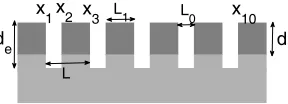
L=x3−x1 for x1 ≤x ≤xm. An example with five grooves (m = 10) is depicted in Fig. 1. For such
a structure, the standard problem is to calculate the transmitted and reflected wave fields for incident waves given in the semi-infinite uniform segmentsx < x1 and x > xm.
L0
d L
1
L d
e
x
3
x
2
x
1 x10
Figure 1. A schematic view of a piecewise uniform waveguide with 5 grooves (m= 10). The thickness of waveguide core is d and the deepness of grooves is de. The width of the “teeth” and “grooves” are L1 andL0, respectively. The period isL=L0+L1.
3. EIGENMODE EXPANSION METHOD
and to model the radiation modes, PMLs [16, 17] can be used to truncate the y variable. Let the y
variable be truncated to the interval (y0, y∗), then, the eigenmodes of the l-th uniform segment satisfy
ρ(l) s
d dy
1
sρ(l) dφ(l)
dy
+k02ε(l)μ(l)φ(l)= [β(l)]2φ(l), y0< y < y∗, (2)
where φ(l) = φ(l)(y) is an eigenfunction, [β(l)]2 the corresponding eigenvalue, β(l) the propagation constant of the eigenmode, and s = s(y) a complex function related to the PMLs (s = 1 only in the PMLs). Furthermore, the eigenfunctions must satisfy some simple homogeneous boundary conditions at y0 andy∗, that is,
φ(l)(y0) =φ(l)(y∗) = 0. (3)
The above eigenvalue problem has an infinite sequence of eigenpairs which are denoted asφ(jl) and βj(l)
for j = 1, 2, . . .. We assume that the fundamental mode of thel-th segment is φ(1l) with propagation
constant β1(l).
In each uniform segment, the wave field can be decomposed as the sum of forward and backward components, and they can be expanded in the transverse eigenmodes. In the l-th segment where 1< l≤m, the wave field is given as
u(x, y) =
∞
j=1 φ(jl)(y)
a(jl)eiβj(l)(x−xl−1)+
bj(l)eiβj(l)(xl−x)
, xl−1< x < xl. (4)
For the first and last segments, the expansions have the following different expressions:
u(x, y) =
∞
j=1
φ(1)j (y)
˜
a(1)j eiβj(1)(x−x1)+b(1)
j eiβ (1)
j (x1−x)
, x < x1, (5)
u(x, y) =
∞
j=1
φj(m+1)(y)
a(jm+1)eiβj(m+1)(x−xm)+ ˜b(m+1)
j eiβ (m+1)
j (xm−x)
, x > xm. (6)
In the above, the coefficients ˜a(1)j and ˜b(jm+1) are given, and they represent the incident waves in the left
and right semi-infinite waveguides, respectively. The unknown coefficients {a(jl) : 2≤ l≤m+ 1, j =
1,2, . . .} and{bj(l) : 1≤l≤m, j = 1,2, . . .} can be solved from the linear system
A
⎡ ⎢ ⎢ ⎢ ⎢ ⎣
b1
a2
.. . bm am+1
⎤ ⎥ ⎥ ⎥ ⎥
⎦=f, (7)
whereal andbl are column vectors foraj(l) andb(jl), respectively. f is related to the incident waves, and
Ais a matrix with a banded structure. Equation (7) can be established from the continuity conditions of uand ρ−1∂xu at x=xl for 1≤l≤m.
4. SCATTERING MATRIX METHOD
The scattering matrix method [6, 18] is often used with EEM to avoid the large linear system (7) and reduce the memory requirement from O(mN2) toO(N2). For a general piecewise uniform waveguide, the scattering matrix method cannot reduce the required number of operations. But if the structure is periodic, it can be accelerated by a recursive-doubling procedure. Then, the number of operations can be reduced to O(N3log
2m). The scattering matrix method calculates the scattering matrix S(x−1, x+m)
satisfying
S(x−1, x+m)
˜ a1
˜ bm+1
=
am+1
b1
, (8)
with ˜a1 and ˜bm+1 as column vectors for coefficients ˜a(1)j and ˜b(jm+1) of the incident waves. If the
structure is periodic, the matrix S(x−1, x+m) can be computed from the scattering matrix for a single
period. A brief summary of the scattering matrix method and the recursive-doubling procedure in given in Appendix A.
5. MODE REDUCTION PROCEDURE
First, we calculate the scattering matrices of individual segments using all numerical eigenmodes. Next, we reduce the size of these scattering matrices, and use them to find a reduced version of the final scattering matrix S(x−1, x+m). For a waveguide grating with periodic feature, we only need to consider
the segment given by x1 < x < x2. The scattering matrix for the considered segment, denoted as S(x−1, x+2), satisfies
S(x−1, x + 2)
˜ a1
˜ b3
=
a3
b1
, (9)
where ˜b3 is a column vector, and coefficients ˜b (3)
j are used in the following expansion
u(x, y) =
∞
j=1
φ(3)j (y)
a(3)j eiβj(3)(x−x2)
+ ˜b(3)j eiβj(3)(x2−x)
, x > x2. (10)
In the fully discretized version, S(x−1, x +
2) is a (2N)×(2N) matrix and can be calculated in O(N3)
operations. If we only keep N∗ modes, then S(x−1, x+2) is approximated by a (2N∗)×(2N∗) matrix,
and it can be used to find a (2N∗) ×(2N∗) approximation of the final scattering matrix S(x−1, x+m)
in O(N3
∗log2m) operations. Therefore, the total number of operations is O(N3) +O(N∗3log2m). In
particular, for largem, a significant speedup may be achieved.
To select the modes, we first normalize the eigenmodes such that
y∗
y0
s(y)
ρ(l)(y)
φ(jl)(y)
2
dy = 1. (11)
For an incident fundamental modeφ(1)1 (y)eiβ (1)
1 (x−x1)(i.e., ˜a1= [1,0, . . . ,0]T and ˜b3 =0), the coefficients
of the transmitted and reflected waves of one period are the first column of matrixS(x−1, x +
2). Letg be
the vector containing the firstN elements of the first column of matrixS(x−1, x+2). We select the modes
based on the magnitudes of the elements of g. More precisely, for an integer N∗ < N, we choose N∗
elements with the largest magnitude in g, and find the mode indices for all these elements, and finally get theN∗ modes that we need to keep. Based on theN∗ selected modes, by keeping the corresponding
row and column elements inS(x−1, x +
2), we could find a (2N∗)×(2N∗) matrix approximatingS(x−1, x + 2).
6. NUMERICAL EXAMPLES
The first example is a modeling exercise of COST 268 [19]. It is about an optical waveguide with a deeply etched short Bragg grating as shown in Fig. 1. The original waveguide is formed by a Si3N4layer
and the substrate are frequency dependent and given in [19]. The Bragg grating is composed of 1024 rectangular grooves with a grating period ofL= 0.43µm. The widths of the “tooth” and “groove” are chosen to be equal, i.e., L0 = L1 = 0.215µm. The groove depth is de = 0.625µm. In all examples,
we assume that an incident fundamental mode is coming from x < x1. In numerical implementation,
the transverse y direction is truncated by PMLs to an interval with length 4.5µm with 2.5µm in the substrate and 1.5µm in the air, and discretized by a fourth-order FD scheme [20] with N = 180 grid points. Fig. 2 shows the absolute values of the first 180 elements in the first column of S(x−1, x
+ 2) at
wavelength λ = 1.55µm. We can see that the values decay very fast with the increasing mode index for both TE and TM cases. Under certain error tolerance, we can discard the modes corresponding to elements with small magnitudes in constructing an approximation to scattering matrixS(x−1, x+m).
0 50 100 150
0 0.5 1
Mode Index
Magnitude
0 50 100 150
0 0.5 1
Magnitude
Figure 2. The absolute value of the first 180 elements in the first column of S(x−1, x+2) in the
first example with wavelength λ= 1.55µm. Top and bottom pictures correspond to TE and TM polarizations, respectively.
1 1.2 1.4 1.6 1.8
0 0.2 0.4 0.6
Wavelength[µm] 0
0.5 1
R, Exact R, N =50
T, Exact T, N =50 TM
TE
*
*
Figure 3. The reflection and transmission spectra calculated by EEM with and without mode reduction technique in the first example. Top figure corresponds to the TE polarization; bottom figure corresponds to the TM polarization.
N∗ = 50 modes are used in the mode reduction
technique.
20 40 60 80 100 10 -5
10 -3 10- 1
N
Error
20 40 60 80 100 10- 6
10- 4 10 -2
N
* *
Figure 4. Error of transmission and reflection computed by EEM with mode reduction technique for different N∗ and N in the first example. Left figure is for transmission of TE polarization at wavelength λ = 1.48µm; right figure is for reflection of TM polarization at wavelength λ = 1.29µm. Blue star, green circle and red triangle are for N = 180, N = 360 and N = 720, respectively.
1 1.2 1.4 1.6 1.8
0 0.5 1
Wavelength[µm] R, Exact R, N =80
T, Exact T, N =80
*
*
To demonstrate the effectiveness of the simulation of wavefields from the proposed mode reduction technique, Fig. 3 shows the reflection and transmission spectra calculated by EEM with and without mode reduction technique. The number of retained modes in mode reduction technique is N∗ = 50.
In this paper, the “exact” results refer to the results computed by EEM without mode reduction technique. We can see that the mode reduction technique can produce very accurate results with less than 30% of the total modes. The largest maximum absolute error of reflection and transmission for TE polarization is 4.3×10⁻³ and 7.0×10⁻⁴, respectively. The largest maximum absolute error for reflection and transmission of TM polarization is 7.0×10⁻⁴ and 6.0×10⁻⁴, respectively. At two fixed wavelengths, error of transmission and reflection computed by EEM with different N∗ and N is shown
in Fig. 4. Generally, high accuracy can be achieved by using less than 30% of the modes.
The second example is a high index contrast optical waveguide as shown in Fig. 1. The thickness of the waveguide core is d = 0.22µm and the depth of the “grooves” is de = d. The width of the “teeth” and “grooves” are L1 = 0.175µm and L0 = 0.135µm, respectively. There are 1024 periods.
The refractive indexes of the waveguide core and substrate are n2 = 3.4 and n3 = 1.45, respectively.
The superstrate is air. In numerical calculation, the transverse y direction is truncated by PMLs to an interval of length 3.08µm with 1.54µm in substrate and 1.32µm in superstrate and discretized by
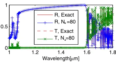
N = 280 grid points. The reflection and transmission spectra for TE polarization calculated by EEM with and without mode reduction technique are given in Fig. 5. The number of retained modes in mode reduction technique is N∗ = 80. The largest maximum absolute error for reflection and transmission is
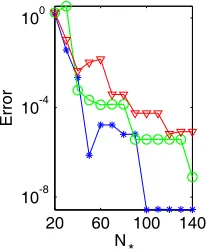
2.5×10⁻⁴. Fig. 6 shows the error of reflection computed by EEM with mode reduction technique with different N∗ and N at wavelength 1.62µm for TE polarization.
20 60 100 140 100
10-4
10-8
N
Error
*
Figure 6. Error of reflection computed by EEM with mode reduction technique with different N∗
and N in the second example at wavelength λ= 1.62µm for TE polarization. Blue star for N = 280, green circle forN = 560 and red triangle for
N = 1120.
1.520 1.53 1.54 1.55 1.56
0.5 1
Wavelength[µm]
R, N=280 R, N
*=30
T, N=280 T, N
*=30
Figure 7. The reflection and transmission spectra of the defect waveguide calculated by EEM with and without mode reduction technique for TE polarization in the third example. N∗ = 30 modes are used in the mode reduction technique.
In the third example, we consider a defect structure that has been studied in Section 5.3 in [21]. The defect waveguide contains 8 grooves with the central “tooth” be 1.515µm width. Other parameters are the same as that in the second example. The reflection and transmission spectra calculated by EEM with and without mode reduction technique for TE polarization are shown in Fig. 7. The transverse direction is discretized by N = 280 grid points, and N∗ = 30 modes are used in the mode reduction technique. The largest maximum absolute error for both reflection and transmission is 1.3×10⁻³ and 3.8×10⁻³, respectively. For such short structures, mode reduction technique could gain high accuracy
with about 10% of the total modes.
7. CONCLUSION
difference method after the transverse direction is truncated by PMLs. This step costsO(N3) operations with N as the number of discrete grid points in transverse direction. Second, the scattering matrix of a single period is computed using the full set of eigenmodes withO(N3) operations. Finally, the most
importantN∗ (N∗ < N) eigenmodes are selected elegantly and used to construct the scattering matrix
of the whole structure by a recursive-doubling procedure. This requires O(N∗3log2m) operations for a structure withmperiods. The total number of operations isO(N3)+O(N∗3log2m). Numerical examples demonstrate that we can obtain a high accuracy withN∗ less than one third of N.
ACKNOWLEDGMENT
This work was partially supported by the National Natural Science Foundation of China (project No. 11201508), the Scientific Research Foundation of Chongqing Technology and Business University (project No. 20125605), the Scientific and Technological Research Program of Chongqing Municipal Education Commission (grant No. KJ130726) and in part by Fudan University under The Talent Recruitment Grant No. IDH1207001, the NSFC No. 61271158, the NSF from Shanghai No. 14ZR1402400.
APPENDIX A. SCATTERING MATRIX METHOD WITH RECURSIVE-DOUBLING
In this section, a brief summery of how to use recursive-doubling procedure to calculate the scattering matrixS(x−1, x+m) of periodic structures is given in [6, 18]. Since the structure is symmetry, the scattering
matrixS(x−1, x +
2) for segmentx1< x < x2 can be written in blocks form as
S(x−1, x+2) =
T R R T
. (A1)
To compute matrices T and R, we first compute the scattering matrix of a single interface. With expressions (5) and (4) truncated to N terms and using the continuity conditions of u at interface
x=x1, a (2N)×(2N) scattering matrix S(x−1, x+1) for interface x=x1 can be obtained as
S(x−1, x + 1)
˜ a1
˜ b2
=
S(1)11 S(1)12 S(1)21 S(1)22
˜ a1
˜ b2
=
a2
b1
, (A2)
where ˜b2 = Γ2b2, and Γ2 is a N ×N diagonal matrix with jth diagonal eiL0β (2)
j for j = 1,2, . . . , N.
Similarly, form Equations (4) and (10) and the continuity conditions ofuatx=x2, we have a scattering
matrixS(x−2, x +
2) at interfacex=x2 as
S(x−2, x+2)
˜ a2
˜ b3
=
S(2)11 S(2)12 S(2)21 S(2)22
˜ a2
˜ b3
=
a3
b2
, (A3)
where ˜a2=Γ2a2. Eliminating ˜a2 and ˜b2 form Equations (A2) and (A3), we have
T =S(1)22Γ2PS(2)22, R=S (1) 21 +S
(1)
22Γ2PS(2)21Γ2S(1)11, (A4)
whereP = (I−S(2)21Γ2S(1)12Γ2)−1 and I is the identity matrix.
To compute scattering matrixS(x−1, x+m) of the whole periodic structure, we first rewrite it as
S(x−1, x + m) =
Tm Rm Rm Tm
. (A5)
If the number of segments m is a power of 2, i.e., m = 2K, let T1 = T and R1 = R, the
recursive-doubling procedure is given as
T2k+1 =T2kΓ1P2kT2k, R2k+1 =R2k+T2kΓ1P2kR2kΓ1T2k, (A6)
for k = 0,2, . . . , K −1, where Γ1 is a N ×N diagonal matrix with the jth diagonal element eiL1β (1)
j
for j = 1,2. . . , N and P2k = (I−R2kΓ1R2kΓ1)−1. The total number of operations is O(N3K), i.e., O(N3log
REFERENCES
1. Liu, Q. H. and W. C. Chew, “Analysis of discontinuities in planar dielectric waveguides: An eigenmode propagation method,” IEEE Transcations on Microwave Theory and Techniques, Vol. 39, No. 3, 422–430, 1991.
2. Sztefka, G. and H. P. Nolting, “Bidirectional eigenmode propagation for large refractive index steps,” IEEE Photonics Technology Letters, Vol. 5, 554–557, 1993.
3. Willems, J., J. Haes, and R. Baets, “The bidirectional mode expansion method for 2-dimensional wave-guides — the TM case,” Optical and Quantum Electronics, Vol. 27, 995–1007, 1995.
4. Helfert, S. F. and R. Pregla, “ Efficient analysis of periodic structures,” Journal of Lightwave Technology, Vol. 16, 1694–1702, 1998.
5. Bienstmain, P. and R. Baets, “Optical modelling of photonic crystals and VCSELs using eigenmode expansion and perfectly matched layers,” Opt. Quant. Electron., Vol. 33, 327–341, 2001.
6. Silberstein, E., P. Lalanne, J. P. Hugonim, and Q. Cao, “Use of grating theories in integrated optics,” J. Opt. Soc. Am. A, Vol. 18, 2865–2875, 2001.
7. Ctyrok´˘ y, J., “Improved bidirectional mode expansion propagation algorithm based on Fourier series,”Journal of Lightwave Technology, Vol. 25, No. 9, 2321–2330, 2007.
8. Rao, H., R. Scarmozzino, and R. M. Osgood, “A bidirectional beam propagation method for multiple dielectric interfaces,” IEEE Photonics Technology Letters, Vol. 11, No. 7, 830–832, 1999. 9. Ho P. L. and Y. Y. Lu, “A stable bidirectional propagation method based on scattering operators,”
IEEE Photon. Technol. Lett., Vol. 13, No. 12, 1316–1318, 2001.
10. Ho P. L. and Y. Y. Lu, “A bidirectional beam propagation method for periodic waveguides,”IEEE Photon. Technol. Lett., Vol. 14, 325–327, Mar. 2002.
11. Yuan, L. and Y. Y. Lu, “An efficient bidirectional propagation method based on Dirichlet-to-Neumann maps,” IEEE Photonics Technology Letters, Vol. 18, 1967–1969, Sep. 2006.
12. Yuan, L. and Y. Y. Lu, “A recursive doubling Dirichlet-to-Neumann map method for periodic waveguides,” Journal of Lightwave Technology, Vol. 25, 3649–3656, Nov. 2007.
13. Taflove, A. and S. C. Hagness,Computational Electrodynamics: The Finite-difference Time-domain Method, 2nd edition, Artech House, 2000.
14. Mendoza-Su´arez, A., F. Villa-Villa, and J. A. Gaspar-Armenta, “Numerical method based on the solution of integral equations for the calculation of the band structure and reflectance of one- and two-dimensional photonic crystals,” J. Opt. Soc. Am. B, Vol. 23, No. 10, 2249–2256, 2006.
15. Mendoza-Su´arez, A., H. P´erez-Aguilar, and F. Villa-Villa, “Optical response of a perfect conductor waveguide that behaves as a photonic crystal,” Progress In Electromagnetics Research, Vol. 121, 433–452, 2011.
16. Berenger, J. P., “A perfectly matched layer for the absorption of electromagnetic-waves,” J. Comput. Phys.,Vol. 114, No. 2, 185–200, 1994.
17. Chew, W. C. and W. H. Weedon, “A 3D perfectly matched medium from modified Maxwell’s equations with stretched coordinates,” Microwave and Optical Technology Letters, Vol. 7, No. 13, 599–604, 1994.
18. Li, L., “Formulation and comparison of two recursive matrix algorithms for modeling layered diffraction gratings,”Journal of Optical Society of America A, Vol. 13, No. 5, 1024–1035, 1996. 19. Ctyrok´˘ y, J., S. Helfert, R. Pregla, P. Bienstman, R. Baets, R. De Ridder, R. Stoffer, G. Klaasse,
J. Petr´a˘cek, P. Lalanne, J.-P. Hugonin, and R. M. De La Rue, “Bragg waveguide grating as a 1D photonic band gap structure: COST 268 modelling task,” Optical and Quantum Electronics, Vol. 34, 455–470, 2002.
20. Chiou, Y. P., Y. C. Chiang, and H. C. Chang, “Improved three-points formulas considering the interface conditions in the finite-difference analysis of step-index optical devices,” J. Lightwave Technology, Vol. 18, No. 2, 243–251, 2000.