The Dark SIDH of Isogenies

(1)

The Dark SIDH of Isogenies

Paul Bottinelli, Victoria de Quehen, Chris Leonardi, Anton Mosunov, Filip Pawlega, and Milap Sheth

ISARA Corporation, Waterloo, Canada

{paul.bottinelli,victoria.dequehen,chris.leonardi,filip.pawlega,milap.sheth}@isara.com [email protected]

Abstract. Many isogeny-based cryptosystems are believed to rely on the hardness of the Supersingular Decision Diffie-Hellman (SSDDH) problem. However, most cryptanalytic efforts have treated the hardness of this problem as being equivalent to the more generic supersingular`e-isogeny problem — an established hard problem in number theory.

In this work, we shine some light on the possibility that the combination of two additional pieces of information given in practical SSDDH instances — the image of the torsion subgroup, and the starting curve’s endomorphism ring — can lead to better attacks cryptosystems relying on this assumption. We show that SIKE/SIDH are secure against our techniques. However, in certain settings, e.g., multi-party protocols, our results may suggest a larger gap between the security of these cryptosystems and the`e_-isogeny problem.

(2)

By the early 2000s, the elliptic curve discrete logarithm problem had become the primary choice for concrete instantiations of fundamental cryptographic protocols, and enabled many new advancements in the field. Looking closer at the structure of, and relationship between elliptic curve groups gave way to a natural generalization: rather than using scalar multiplication maps, cyclic isogenies could be used to achieve similar algebraic properties [9, 20, 22]. In 2006, Charles, Goren and Lauter [5] introduced the first cryptographic primitive (a hash function) relying on the hardness of finding isogenies betweensupersingular

elliptic curves. Their work introduced the “supersingular `e_{-isogeny problem”} in a cryptographic context, and provided heuristic analysis of its hardness by studying the structure of the set of all possible isogenies between supersingular elliptic curves.

In 2011, supersingular isogeny-based cryptography received renewed attention with the demonstration of a quantum sub-exponential algorithm for finding isoge-nies between ordinary elliptic curves by Childs, Jao, and Soukharev [7]. Motivated by avoiding this attack, De Feo and Jao [13] revisited the `-isogeny graph of supersingular curves first considered in [5], and introduced the Supersingular Isogeny Diffie-Hellman protocol (SIDH).

In order to overcome a technical obstacle in constructing the protocol, the public keys in SIDH include the images of certain torsion points under the (pri-vate) isogenies. The Supersingular Isogeny Decisional Diffie-Hellman assumption (SSDDH) – and its computational versions Supersingular Isogeny Computational Diffie-Hellman assumption (SSCDH) and Computational Supersingular Isogeny assumption (CSSI) – were introduced to prove the security of this protocol given the additional information. The Supersingular Key Encapsulation Mech-anism SIKE [12], currently being considered for standardization in the NIST Post-Quantum Standardization Process [6], also relies on the hardness of the relatively-new SSDDH problem on a fixed starting curve. This new computa-tional assumption was presumed to be equivalent to the supersingular`e_-isogeny problem.

The distinction between the SSDDH assumption and the`e_{-isogeny problem} (namely, that torsion point images of private kernels are revealed) was first exploited in 2016, when the prominent work due to Galbraith, Petit, Silva, and Ti [11] (later referred to as “GPST”) presented an active attack on the use of static-keys in SIDH.

(4)

security of SIKE. However, their work demonstrated that the problem of finding endomorphism rings is intricately linked to the security of SIKE.

Since then, numerous works have shown constructions of additional primitives assuming the hardness of classical`e_{-isogeny problems, SSDDH, and strengthened} variants of SSDDH. Most of the current best-known attacks [1,24] on SIDH/SIKE find direct solutions to the`e_{-isogeny problem. Recently, the authors in [14] have} also suggested that the quantum attack of Biasse et al. [4] exploiting the algebraic structure of supersingular elliptic curves defined overFp might be better than the often cited generic quantum claw-finding attack [24].

In 2017, Petit [17] described a passive polynomial time algorithm for solving the CSSI problem on two non-SIKE parameter sets, the first work to utilize both the image of the torsion points, and the knowledge of the endomorphism ring of the starting curve. In the first variant, one party reveals drastically more torsion information than in SIDH/SIKE (like in multi-party settings [3]), and in the other variant both parties work in torsion subgroups larger thanp2 _(where_p_is

the characteristic of the field) and reveal slightly more torsion information than in SIDH/SIKE. The novelty of the work we present in this paper is that we arrive at potentially stronger results in the same vein of that work, but using different methods. More specifically, we aim to answer the following question: is there an offline algorithm which solves CSSI by repeatedly restricting the search-space by a non-negligible factor, e.g., apassive counterpart to [11]?

1.1 Our Contributions and Organization of the Paper

This work constitutes an independent line of research into non-generic attacks on the instantiations of the CSSI problem. We describe a reduction between the security of SIDH-like protocols and the CSSI problem on certain starting elliptic curves. Given an oracle for this new problem, we present a passive algorithm which iteratively shrinks the search space for solutions to the CSSI problem, which corresponds to recovering a private key (isogeny) in protocols relying on the CSSI assumption. Our approach exploits the knowledge of the images of the private isogeny on a torsion subgroup, and the structure of the endomorphism ring of the starting curve.

In Section 2 we review the hardness assumptions used to establish the security of SIKE, and in Section 3 we give a technical overview of the work in this document. Similar to our reduction, the “GPST attack” [11] iteratively gives malformed public keys to halve the search space. Our methods can be interpreted as a generalization of the underlying ideas implicit in the GPST attack (see Table 1 for a comparison). While the best-known attacks deal with elliptic curves and other rich structures, our analysis interprets torsion points asvectors and endomorphisms as matrices, and applies techniques from linear algebra. We formulate the GPST attack using this terminology in Section 4.

(5)

in a novel way, called atriangular kernel. Thus, we show a reduction between the CSSI problem and the problem of finding desirable endomorphisms.

Once we fix a specific (starting) elliptic curve, constructing such endomor-phisms essentially reduces to solving a particular quadratic form. In Section 6, we make explicit the reduction between the security of SIDH/SIKE variants and the problem of finding (desirable) solutions to this quadratic form. An important result of our investigations, which we show in Section 7, is that SIKE is secure against our cryptanalysis.

Section 8 explores whether these desirable endomorphisms exist in the multi-party setting (e.g., group key agreements [3]). We provide arguments that suggest the security of the standard 3-party and 4-party cases may be significantly less than currently believed. Specifically, we provide heuristic evidence about the existence of desirable endomorphisms for our attacks in the 4-party setting.

Section 9 examines the tradeoff between the runtime of our algorithm and the amount of information each desirable endomorphism provides. Section 10 focuses on improving the algorithm so that it requires fewer desirable endomorphisms. Informally, we achieve this by learning the images of the private isogeny on additional torsion points.

Finally, in Section 11, we introduce a modified version of SIKE (called SITH) which relies on a qualitatively weaker security hypothesis. We end with our conclusions and future work in Section 12. This work shares a similar conclusion to that of Petit [17], which presented a passive polynomial-time algorithm to solve two variants of the CSSI problem.

2 Preliminaries

As we will be working in a broader setting than SIKE, Section 2.1 introduces the necessary notation for general isogeny-based key exchanges, and Section 2.2 reviews the hard problems upon which the security of these key exchanges is based.

2.1 Notation

Throughout, we will assume a generalization of the SIKE setup. In particular, let Fq denote a finite field withq elements, where q=p2 for some primepof the formp=N1N2−1,for coprime positive integersN1 andN2. The security

parameter of isogeny-based cryptosystems is λ= logp. In much of Sections 7 and 8 we will be assumingp≡3 (mod 4).In this case, as_Fp2 ∼=_F_p[x]/hx2+ 1i,

we can represent elements in_Fp2 asu+vi, wherei2=−1, for someu, v∈_F_p.

We will letE(_F) denote a supersingular elliptic curveE over a field_F. As well, letE[N] denote the subgroup ofN-torsion points over the algebraic closure

Fq, and let [N] denote the isogeny that acts as scalar multiplication byN. For anyN ∈_Z, wherep_-N, the subgroup E[N]∼=Z/NZ×Z/NZ. We fix

(6)

Let RA =PA+ [rA]·QA for some number rA ∈ {0, . . . , NA−1}, and let φA : E → EA be an isogeny with ker(φA) = hRAi. Alice will be the static initiator in the key exchange, whoseprivate key is rA. We refer toRA as her

private point, which generates the kernel of herprivate isogeny φA. Herpublic key is (φA(E), φA(PB), φA(QB)).

Occasionally, we will also use an isogenyφB :E →EB, where ker(φB) =

hPB+ [rB]·QBifor some numberrB∈ {0, . . . , NB−1}. Bob will be the responder in the key exchange, whose private key is rB. We refer toRB as his private

point, which generates the kernel of his private isogeny φB. Hispublic key is (φB(E), φB(PA), φB(QA)).

Definition 2.1. Letφ:E→E0 _{be an isogeny. Then}_φ_{is said to be}_cyclic_when

there is no integer m6={±1} and isogenyψsuch thatφ= [m]·ψ.

We denote the action of the isogenyφrestricted to theN-torsion points by φ|_E_[_N_],typically with respect to a given basis{P, Q} forE[N]. Finally,φbwill denote the dual of an isogenyφ.

Let End(E) denote the endomorphism ring ofE. SinceE is supersingular, we can write End(E) as aZ-module generated by some basis of endomorphisms {b1, b2, b3, b4}.

For a natural numberN and linear transformation M onE[N], let

Eig_NM ={R∈E[N] :|R|=N,hM(R)i ⊂ hRi}.

We refer to this as the N-eigenspace of M, and call a torsion point R an

eigenvector of M if it is in Eig_N(M). For an endomorphism φC and natural number N, let

Eig_N(φC) ={R∈E[N] :|R|=N,hφC(R)i ⊂ hRi}.

We refer to this as the N-eigenspace of φC, and call a torsion point R an

eigenvector ofφC if it is in EigN(φC) for some natural numberN. Notice that if gcd(degφC, N) = 1 andR∈EigN(φC), thenhRi=hφC(R)i.

LetH(ρ) be theinformation entropy of a binary probability eventρ. Then the expected information content of ρ is H(ρ) bits, and can be computed as follows

H(ρ) =ρlog2(1/ρ) + (1−ρ) log2(1/(1−ρ)).

2.2 Hard Isogeny Problems

As we discussed earlier, most of the current best-known attacks [1, 24] on SIDH/SIKE find direct solutions to the`e_{-isogeny problem:}

Problem 2.2 (`e_{-Isogeny Problem).} _{Suppose there exists an isogeny} _φ _:

E→E0 whose kernel is generated by R∈E[`e_{]. If you are only given}_E _and_E0_, the problem is to findhRi.

(7)

Problem 2.3 (Supersingular Decision Diffie-Hellman (SSDDH)

Prob-lem). Given a tuple sampled with probability 1/2 from one of the following two

distributions:

1. (EA,EB,φA(PB),φA(QB),φB(PA),φB(QA),EAB), generated via the SIDH protocol and

EAB∼=E0/hPA+ [rA]·QA, PB+ [rB]·QBi,

2. (EA,EB,φA(PB),φA(QB),φB(PA),φB(QA),EC), where everything except EC is generated via the SIDH protocol and

EC ∼=E0/hPA+ [r0A]·QA, PB+ [r0B]·QBi,

wherer0_Aandr_B0 are chosen at random from_Z/N_1Zand_Z/N_2Z,respectively, determine from which distribution the tuple is sampled.

A computational variant of this problem was introduced by Jao and De Feo in [13].

Problem 2.4 (Supersingular Computational Diffie-Hellman (SSCDH)

Problem). LetφA:E0→EAbe an isogeny whose kernel is equal tohPA+ [rA]·

QAi, and letφB :E0→EBbe an isogeny whose kernel is equal tohPB+[rB]·QBi, whererA(respectivelyrB) is chosen at random fromZ/N1Z(respectivelyZ/N2Z).

Given the curvesEA,EB, and the pointsφA(PB), φA(QB), φB(PA), φB(QA), find thej-invariant ofE0/hPA+ [rA]·QA, PB+ [rB]·QBi.

SSDDH reduces to SSCDH in the obvious way, and the converse is true as well [26]. Both the decisional and computational Diffie-Hellman assumptions depend on the following computational problem in the obvious way.

Problem 2.5 (Computational Supersingular Isogeny (CSSI) Problem).

Let E0 be a supersingular elliptic curve, and let φ : E0 → EA be an isogeny whose kernel is generated byhPA+ [rA]·QAifor a randomrA∈Z/N1Z, over Fp2 wherep=N₁N₂−1 is a prime such that gcd(N₁, N₂) = 1. GivenE_A and

the action ofφonE0[N2], findrA.

This work aims to study the security of SIDH/SIKE instances by solving the CSSI Problem, which in turn solves the SSCDH and SSDDH problems.

The security of the NIST Round 1 version of SIKE [6] is based on an in-stantiation of the SSDDH problem at the elliptic curveE0 :y2 =x3+xwith

j-invariant 1728. The endomorphism ring of this elliptic curve is known, and it has many endomorphisms with small norm. It is the knowledge of the core structure of the endomorphism ring of the starting elliptic curve E0, along with

(8)

3 Technical Preview

Constructing public-key cryptosystems like SIDH relying on the hardness of SSDDH can be done by viewing an isogeny as a private key, and an image curve (and torsion points) under that isogeny as the public key. Appendix A.1 presents numerous approaches for passive attacks on SIDH that have been presented in the literature, such as the generic claw-finding algorithms from Tani [24], a quantum algorithm performing unstructured searches through an algebraically constrained space of candidate solutions by Biasse, Jao and Sankar [4], and the work by Petit [17] which showed a relationship between the hardness of multi-party SIDH-like protocols and solving certain quadratic forms.

While we study similar concepts as this last attack, our approach is structurally different, as we draw inspiration from theactiveGPST attack [11], which showed why SIDH is not IND-CCA secure. See Table 1 for a comparison between this work and the GPST attack. For this discussion let us assume that Bob is a dishonest party wishing to discover the other party’s, Alice’s, private key.

In the standard SIDH protocol, Bob is required to send particular points derived from his private isogeny during the run of the protocol. In the GPST attack (which we describe in more detail in Section 4.1), Bob, acting as an attacker, repeatedly sends a specially crafted linear combination of his points instead.

Bob’s correct points form a basis ofEB[N1], as do his malicious points. We

will consider the change of basis matrix between these bases. The main idea behind the GPST attack is that, with probability 1/2, Alice is able to reconstruct the correct isogeny given Bob’s malicious points. Whether or not this second isogeny of hers is constructed correctly gives Bob information about Alice’s private key, and this information is completely determined by the change of basis matrix that Bob used.

In our methods, the attacker uses an endomorphism on the starting curve instead of a change of basis matrix. More specifically, we show that given a particular endomorphism, the attacker can discover information about Alice’s private point.

Contrary to the GPST attack, we provide an reduction which requires access todesirable endomorphisms. Hence, for our reduction to result in a useful attack we need i) to obtain a non-negligible amount of information about Alice’s private point during each iteration, and ii) that the cost of each iteration only requires reasonably bounded effort. These two goals add different restrictions on the type of endomorphisms that we consider.

We first study the amount of information determined at each iteration. In the GPST attack, the change of basis matrix between Bob’s correct points and his malformed points can be thought of as acting on the subgroupE[N1] containing

Alice’s private point (as described in Section 4). In this interpretation, if Alice’s private point is an eigenvector of this change of basis matrix, then the protocol succeeds, otherwise (with overwhelming probability) the protocol fails.

(9)

information of Alice’s private point during each iteration. Our observation is that the protocol succeeds exactly half the time because Bob chooses a change of basis matrix such that Alice’s private point is an eigenvector exactly half of the time. More generally, if Alice’s private point is an eigenvector of the change of basis matrix with a probabilityρ <1/2, then Bob is expected to discoverH(ρ) bits of information about Alice’s private key (the information entropy ofρ). Based on the success or failure of the protocol with the malformed image points, Bob can adapt the change of basis matrix, and repeat a similar procedure, learningH(ρ) bits of Alice’s private key with each iteration.

GPST attack Our work

Mode Active Passive

Algorithm type Attack Reduction (requires Oracle queries) Target Static SIDH Instantiated SSDDH

Objects Change of basis matrices Endomorphisms Bits recovered 1 bit H(ρ) bits

Runtime Poly-time Depends on degree of endomorphism Memory Poly-space Poly-space

Table 1: Comparison of the GPST attack with our work.

Instead of a change of basis matrix, our methods assume that the reduction has access to desirable endomorphisms on the starting curve. However, such endomorphisms also act as a matrix on the subspace that contains all of Alice’s possible private points. As with the GPST attack, if Alice’s private point is an eigenvector of the endomorphism with a high probabilityρ≤1/2, then, using our methods, the attacker learns close to one bit of information of Alice’s private key. By repeating this attack with different endomorphisms, the attacker can discover Alice’s private key. Therefore, in order to gain a significant amount of information about Alice’s private point, the attacker uses endomorphisms where Alice’s private point is an eigenvector of the endomorphisms with a reasonably high probability.

Given an endomorphism (with many eigenvectors), the algorithm in our reduction requires the adversary to construct an isogeny on Alice’s curve of the same degree. The runtime of our algorithm depends on the time it takes the attacker to construct this isogeny. As the endomorphism and the related isogeny have the same degree, the difficulty of constructing this related isogeny roughly grows with the degree of the endomorphism. Thus, we are interested in using endomorphisms that have particular degrees.

Alice’s public key includes the image under her private isogeny of the subspace of points whose order dividesN2= 3b. As we will see in Section 5, this additional

information makes it easy to construct an isogeny on Alice’s curve EAthat is the composition of three isogenies, where the first and last isogenies have degrees dividing N2 and the middle isogeny is ideally of small degree. Thus, we are

interested in endomorphisms (on the starting curve) whose degrees have the form kL whereL|N2

(10)

that section is the notion of a triangular kernel (see Section 5), which is a triple of points that generates the isogenies in this decomposition.

In summary, for our reduction to be practical, it requires endomorphisms on the starting curve with large eigenspaces and certain conditions on the degrees. As above, by repeating this procedure with many endomorphisms, Alice’s private key can be recovered.

In order to investigate the existence of desirable endomorphism, we can exploit the knowledge of the endomorphism ring of the starting curve of SIDH/SIKE. In this case, the problem of finding desirable endomorphisms is reduced to solving a particular quadratic form. By studying the quadratic forms arising in the SIKE setting, we are able to show the following non-existence result: no desirable endomorphisms exist that make the above attack strategy on SIKE more efficient than known attacks. A similar result holds for the standard parameterizations of SIDH.

However, investigating the quadratic form arising in multi-party isogeny-based protocols (where the structure of the prime is modified to p=N1·. . .·Nn−1, for coprime natural numbersN1, . . . , Nn) leads us to heuristic arguments about

the existence of desirable endomorphisms for these cases. This suggests that there exist endomorphisms that could be used to give an improved attack in the 4-party case. That being said, it is unclear how difficult it is to construct such endomorphisms. In the 3-party case we do not have heuristics for why such endomorphisms should exist, but if they do, then our cryptanalysis improves upon the best-known attacks in the literature.

We also show a trade-off between the amount of information about Alice’s private point that an endomorphism reveals, and how efficiently this information can be determined. This trade-off is between the size of the eigenspace of the desirable endomorphism and the degree of the endomorphism on the image curve (specifically, the part of the endomorphism that needs to be searched for exhaustively).

Additionally, we show that if Alice’s key is found to be in the eigenspace of two (independent) desirable endomorphisms, then we can improve our reduction. In particular, these endomorphisms can be used to find information about the image of torsion points on the starting curve under Alice’s private isogeny. Thus, instead of just using the torsion information in Alice’s public key, we have additional torsion information to exploit.

We conclude this paper with a recommendation consisting of a SIKE-like protocol which randomizes the starting curve, and thus avoids any potential future attack that utilizes the known endomorphism ring of the starting curve.

4 Interpreting Private Keys as Eigenvectors

(11)

point is an eigenvector of a change of basis matrix. In Section 4.2 we replace the matrices in the GPST attack by endomorphisms, and this gives us our first results concerning whether or not a party’s private point is an eigenvector of an endomorphism.

4.1 The GPST Active Attack on SIDH

In 2015, Galbraith, Petit, Shani and Ti [11] introduced an active attack on users with static SIDH keys who do not use a Fujisaki-Okamoto type transformation [16] to verify the other communicating party’s public key. This attack was originally formulated in terms of Bob’s public key containing a malicious linear combination of the points φB(PA) and φB(QA). It has since been observed that Bob is, in essence, altering the points of φB(PA) and φB(QA) using a change of basis matrix [25], where the matrix has entries in _Z/N_1Z and is chosen to have determinant 1 to avoid detection (using the Weil-pairing test [21,§III.8]). In this subsection, we will rephrase the GPST attack by noticing that these change of basis matrices are designed to have large eigenspaces.

Notation 4.1. Throughout this section,p= 2a3b−1,whereN1= 2a≈3b=N2.

In this subsection we assume that the adversary, Bob, is trying to find Alice’s private key. A similar analysis could be done to attack Bob’s private key (see [11] for the details).

Specifically, in this attack, Bob maliciously alters the image pointsφB(PA) andφB(QA) to another linear combination of those points before sending them to Alice. Depending on whether or not Alice and Bob compute the same shared secret key, by observing if Alice terminates the session, Bob can deduce one bit of information of Alice’s private keyrA. By repeating this attack withndifferent linear combinations of the image pointsφB(PA) andφB(QA), Bob can discover allnbits of Alice’s private key. This attack is devastating against static keys.

We provide the first iteration in the GPST attack as an illustration.

Attack (GPST Attack Iteration 1).Suppose that instead of sending Alice his

public key EB, φB(PA), φB(QA),Bob maliciously sendsEB, φB(PA), φB(QA) + [2a−1]·φB(PA). Then Alice follows the protocol and calculatesψ0_Awith kernel

hφB(PA) + [rA]·(φB(QA) + [2a−1]·φB(PA))i, although Alice believes that she is calculatingψA with kernel

hφB(PA) + [rA]·φB(QA)i. Meanwhile, Bob calculates ψB with kernel

hφA(PB) + [rB]·φA(QB)i.

(12)

The first iteration reveals a single bit of information about Alice’s private key. In each of the followingn iterations of the GPST attack, Bob adaptively adjusts the linear combination of points in his public key to reveal additional bits of Alice’s private key.

It has been observed that adaptively adjusting the linear combination of points is the same as altering the points ofφB(PA) andφB(QA) using a change of basis matrix (i.e., an invertible linear transformation) [25]. However, what has not been previously observed is that the GPST attack is possible because Bob uses change of basis matrices with large eigenspaces.

Along these lines, a better way to think of the GPST attack is that it exploits whether or not Alice’s secret kernel, kerφA,is invariant under particular change of basis matrices to determinerA. We state this reinterpretation of the GPST attack in the language of linear algebra in the following discussion. This perspective will be useful in Section 5, where we will use similar language to describe potential offline attacks where Alice’s kernel may be invariant under some particular endomorphisms.

Remark 4.2. Given a linear mapM onE[N], a subgroupGofE[N],and an

isogeny φB with gcd(degφB, N) = 1, if M(G) = G, then the isogenies with kernelshφB(G)iandhφB(M(G))iare equal.

The following notation will transform Remark 4.2 into the framework of the GPST attack (see Proposition 4.5).

Notation 4.3. Suppose Bob chooses a linear transformationM onE[2a_{]. We}

will representM as a matrix in SL2(Z/2aZ) with respect to the basis{PA, QA}. We also representPA+ [rA]·QA as the vectorr1A

, andφB(PA) + [rA]·φB(QA) asφB

1

rA

.

When Bob sends the malicious points to Alice, he is actually using a change of basis matrix to send a different basis ofEB[2a_]_.

Lemma 4.4. If M is an invertible matrix acting onE[2a_]_{, and}_R _{is an}

eigen-vector of M, thenM(hRi) =hRi.

Proof. SinceM is invertible,|M(R)|=|R|. ThusM(hRi) =hRi. Substituting Lemma 4.4 into Remark 4.2 gives us the following proposition, which is the essence of the GPST attack. To make the GPST attack practical the change of basis matrices are chosen to have a high percentage of eigenvectors.

Proposition 4.5. SupposeM is an invertible matrix acting onE[2a_]_{. If} 1

rA

is an eigenvector ofM, then the isogenyψAwhose kernel is generated byφB

1

rA

is equal to the isogenyψ0_A whose kernel is generated by φB M 1

rA

.

Proof. LettingR= 1

rA

in Lemma 4.4, we find thatM(hRi) =hRi.The result

(13)

To see how Proposition 4.5 provides a new interpretation of the GPST attack, notice that in Iteration 1 of the attack, if 1

rA

is an eigenvector ofM = 1 0 2a−11

, then ψA = ψA0 (the converse is almost always true). Iteration 1 is efficient because Alice’s private key is an eigenvector ofM with probability 1/2. Thus, this iteration allows the attacker to gain a bit of information about Alice’s private key. The change of basis matrix M in each successive iteration in the GPST attack is adaptively chosen so that Alice’s private key is an eigenvector ofM with probability 1/2. This allows the attacker to gain an additional bit of information about Alice’s key per iteration.

The central idea of this paper is to replace the change of basis matrix in Proposition 4.5 by an endomorphism with many eigenvalues, and thus design an offline algorithm which repeatedly restricts the search-space for recovering a private isogeny in SIDH-like protocols.

4.2 GPST-Inspired Cryptanalysis

We now describe a first attempt at generalizing the GPST attack to the language of endomorphisms. Although our ideas were inspired by the active GPST attack, our aim differs in that our work is towards an offline attack on private keys; that is, our methods do not require any participation from Alice after she provides her public key, nor multiple interactions with her. Unless otherwise specified, we will aim to attack Alice’s private key, although our methods can be applied to any party.

We note that the approach given in this subsection is not meant to be practical and certainly is not useful in the SIKE setting. However, it presents the basic ideas upon which the rest of this work is built. Specifically, although this subsection does not use the (image) points provided in Alice’s public key, a more practical approach of attacking isogeny-based algorithms is presented in Section 5 that does utilize these points.

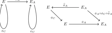
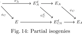
The attacker chooses a particular endomorphismφConE that will mimic the role the matrixM played in the GPST attack, as presented in Section 4.1. We introduce the following notation related toφCthat distinguishes the commutative diagram in Figure 1 as being different from the usual SIDH setup (see Figure 20). This endomorphismφC should be thought of as different fromφBfor two reasons: it is an endomorphism (an isogeny fromE to itself), and it will not be used as part of an SIDH key exchange.

Notation 4.6. In addition to the notation of Section 2.1, let φC be a cyclic

endomorphism onEof degreekthat is generated by a pointRCinE(Fp2), where

gcd(k, N1) = 1.

Let{PC, QC}denote a basis forE[k]. Without loss of generality we can assume RC =PC+[rC]·QCfor somerC. LetψCdenote the isogeny onEAwith the kernel

hφA(RC)i, andψAC denote the isogeny onE with kernelhφC(PA+ [rA]·QA)i, as shown in Figure 1. (Here the superscriptC inψC

(14)

AsφC acts as a linear transformation onE[N1], we can letM ∈SL2(Z/N1Z)

model the action ofφC onE[N1] with respect to the basis{PA, QA}. LetECA

be the image ofψC, and letEAC be the image ofψCA.

As gcd(k,degφA) = 1, the matrix M acts on {PA, QA} as an (invertible) change of basis matrix. Also, as gcd(k, N1) = 1,the square in Figure 1 commutes;

that is,ψC◦φA=ψCA◦φC.

E EA

E EAC∼=ECA

φA

φC

ψC

ψC A

Fig. 1: Commutative diagram with endomorphismφC

With this new notation, we observe the following proposition (similar to Proposition 4.5). Proposition 4.7 will allow us to replace the active part of the GPST attack with an offline computation.

Proposition 4.7. Suppose PA + [rA]·QA is a point of order N1 on E and

φA:E→EA is an isogeny with kernelhPA+ [rA]·QAi. IfPA+ [rA]·QA= 1

rA

is an eigenvector with respect to some endomorphism on E of degree k, with

gcd(k, N1) = 1, then there exists an endomorphism on EA of degreek.

Proof. SupposeφCis an endomorphism onEof degreek, such that Alice’s private pointPA+ [rA]·QA is an eigenvector with respect toφC. As gcd(k, N1) = 1,

we see thatφC acts as an invertible linear transformation onE[N1]. Thus by

Lemma 4.4

hPA+ [rA]·QAi=φC(hPA+ [rA]·QAi).

AsφAhas kernelhPA+ [rA]·QAiandψCA has kernelφC(hPA+ [rA]·QAi) (see Figure 1), we see thatφA∼=ψCA. Thus

ECA∼=EAC=ψAC(E)∼=φA(E) =EA.

Therefore,ψC is an endomorphism onEA of degreek. We now explicitly describe the kernel of this endomorphism for later use.

Corollary 4.8. IfRA is an eigenvector ofφC, then the endomorphism of degree

k from Proposition 4.7 has kernelφA(kerφC).

If k = degφC is small enough to allow us to brute-force the computation of all codomain j-invariants of allk-isogenies fromEA, then it is easy to use Proposition 4.7 to test if r1A

is an eigenvector of φC or not. This is made concrete in the following theorem.

Theorem 4.9. Suppose we are given

1. a supersingular elliptic curveE(_Fp2)such thatp=N₁N₂−1 for coprimeN₁

andN2,

(15)

3. ksuch that there exists a k-endomorphismφC of E, where gcd(k, N1) = 1

andk < N1.

Then there exists a (classical) algorithm with worst case runtimeO˜(k3)which decides whether RA∈EigN1(φC)or RA6∈EigN1(φC)with overwhelmingly high

probability. Further, if kis logp-smooth, then the runtime isO˜(√k).

Proof. By Proposition 4.7 and sincek < N1, it follows that we need to examine

the difficulty of testing if EAisk-isogenous toEA. We will examine to the main two computations involved: constructing a field extension for which EA[k] is defined, and then the computation of degreek isogenies.

We begin by discussing the difficulty of finding an appropriate extension. Factoring thek-th division polynomial overFp2will give an irreducible polynomial

of degree k (many exist, but any will suffice) which will give an appropriate field extension to contain allx-coordinates ofEA[k]. The degree of this division polynomial is k2−1

2 and the polynomial requires this much time and space to

compute. Therefore, by [15], finding a root of this polynomial takes ˜O(k3) time. A quadratic extension on this field will then be guaranteed to contain they -coordinates as well, and thus all of EA[k]. However, whenk is, sayD-smooth, this field can be constructed as a tower of extensions, and thus only takes O(Dlogk) =O(log2p) time.

Next we assume the field extension has been constructed. Whenkis prime, constructing all k-isogenies with domain EA using V´elu’s formulas involves computing thek+ 1 isogenies of prime degreekand domain EA. Prime degree isogenies currently requireO(k) operations to compute [27]. This case, therefore, gives us the worst-case bound of O(k2_{), as there are approximately} _k _such

isogenies to check.

Whenkis not prime, claw-finding methods can be applied to improve per-formance. In the case wherek=k1k2 for some logp-smooth positive integers k1

andk2 each approximately of size √

k, then classical claw-finding will require computing O(k1) many isogenies of degreek1 and computingO(k2) isogenies of

degreek2 [13, 5.1], andO( √

k) space. Whenkis logp-smooth, then the isogeny computations themselves areO(logk) which is negligible.

Thus, the worst case for this iteration is whenkis prime where the runtime is ˜

O(k2), and the best case is whenkis logp-smooth where the runtime is ˜O(√k). Observe that ifkis small (say, less than 100,000 [23]) this computation can be performed by checking if the tuple (j(EA), j(EA)) is a root of thekth modular polynomial. Therefore, the runtime of this step is dominated by the cost of creating a field extension, namely ˜O(k3_).

By Proposition 4.7, ifRA is an eigenvector ofφC then the above process will succeed asEAmust have an endomorphism of degreek. IfRAis not an eigenvector, then a false-positive endomorphism may exist, but is highly improbable when

k < N1.

Remark 4.10. As we see from the proof, the best case for this algorithm is ifk

(16)

Suppose that for someρ=ω(1/poly(λ)), there is an endomorphismφC with small degreek, such that the conditions

|E[N1]∩EigN1(φC)| ≤(1−ρ)· |S|, and (1) |E[N1]\EigN1(φC)| ≤(1−ρ)· |S| (2)

hold. By applying the result of Theorem 4.9, we can discover H(ρ) =ρlog2(1/ρ) + (1−ρ) log2(1/(1−ρ))

bits of information about Alice’s key.

Remark 4.11. Although there are matrices onE[N1] (for instance, those used

in the GPST attack, see [11]) that satisfy Conditions 1 and 2, ifphas the standard formp= 2a₃b₋_{1, then there is no endomorphism that satisfies these conditions} with degree k ∈ O(p) (see Corollary A.3). Thus the algorithm referred to in Theorem 4.9 does not give a viable attack on SIDH.

This theorem does, however, provide the basic premise on which the rest of this work is built.

5 Exploiting Endomorphisms

The goal of this section is to prove our first main result, Theorem 5.11, which reduces the security of SIDH/SIKE variants to the problem of finding certain types of endomorphisms of the starting elliptic curve, which we will refer to as

desirable endomorphisms. We will prove the main result of this section by giving a stronger version of the algorithm from Theorem 4.9 which utilizes the torsion group information given in Alice’s public key.

5.1 Triangular Kernels

The input of the algorithm from Theorem 4.9 isE, EA,and kerφC, whereE is a public parameter of the system,EAis part of Alice’s public key, and kerφC is a pre-computed endomorphism with a low degree and many eigenvectors.

However, in isogeny-based key establishments, Alice’s public key contains more information than simplyEA. It also includes the image underφAof a large torsion subgroup, namely φA|_E_[_N_2]. Thus, from Alice’s public key, it is efficient to calculate an isogeny whose kernel is contained inEA[N2]. Moreover, it is faster

(than simply using brute-force) to calculate an isogeny whose kernel has a large intersection withEA[N2]. In this section, we will formalize this idea.

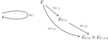
Suppose we have an endomorphismφCof degreeLk, whereL|N2,gcd(k, N1) =

1 and k < N1. Then, there exist isogenies φC,1 and φC,0 on E such that

φC=φbC,0◦φC,1, and kerφC,0= kerφC∩E[N2], see Figure 2. Knowledge of

Al-ice’s public key implies that it is efficient to calculateφA(kerφC,0), and so this fact

(17)

E φC

E

EC,0∼=EC,1

φC,1degk

φC,0degL

Fig. 2: Decomposing endomorphisms (simple)

In fact, not only are we able to improve Theorem 4.9 if gcd(degφC, N2) is

large, but we can improve Theorem 4.9 even more if gcd(degφC, N22) is larger than

gcd(degφC, N2). When this holds, there is another natural way to decompose

φC. This leads us to introduce a new definition that captures the concept behind this type of decomposition.

Definition 5.1. SupposeφCis a cyclic endomorphism ofE. Atriangular

decom-position ofφC with respect toN2 is a triple of cyclic isogeniesφC,0, φC,1, φC,2,

whereφC,0 andφC,1have degrees dividingN2,

φC=φbC,0◦φC,2◦φC,1,

and if gcd(N2,degφC,2)6= 1, then degφC,0= degφC,1=N2.

A triangular kernel of φC with respect to N2 is a triple of torsion points

denoted by ker4φC = (K0, K1, K2), which generate the kernels of the

correspond-ing isogenies of a triangular decomposition, that is, kerφC,i=hKii. Furthermore, letk=|K2|.

Remark 5.2. This representation has the advantage that only the extension

field containing thek-torsion points is needed to write the kernel, instead of the (N2)2k-torsion points. This is becauseK0, K1∈E[N2].

Notice thatK0, K1andK2 could theoretically all be trivial.

Notation 5.3. LetφC,0, φC,1, φC,2denote a triangular decomposition ofφCwith

respect to N2. LetEC,0, EC,1 andEC,1,2 denote the images of φC,0, φC,1, φC,2,

respectively, as illustrated in Figure 3. Then, up to isomorphism,EC,0∼=EC,1,2.

E φC

E

EC,1

EC,0∼=EC,1,2

φC,1

φC,0

φC,2

Fig. 3: Decomposing endomorphisms

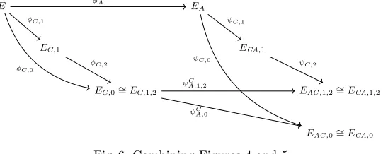
We wish to study a passive adversary’s ability to transfer φC on E over to a corresponding potential endomorphism onEA, using the isogenies in the triangular decomposition ofφC (so that they can test if Alice’s private key is an eigenvector ofφC). In order to calculate the corresponding objects onEA, we introduce notation for additional isogenies.

Notation 5.4. LetψC,0be the isogeny with domainEAand kernelφA(kerφC,0),

andψ_A,C₀be the isogeny with domainEC,0and kernelφC,0(kerφA). Let the images

(18)

Since degφC,0 and degφA are relatively prime,ECA,0∼=EAC,0.

E EA

EC,0 EAC,0∼=ECA,0

φA

φC,0

ψC,0

ψC A,0

Fig. 4: Maps with known kernels

Notation 5.5. We decompose the isogeny with domainEA and kernel equal to

φA(kerφC,2◦φC,1) asψC,2◦ψC,1,where kerψC,1=φA(kerφC,1) and kerψC,2=

ψC,1◦φA(kerφC,2). LetψA,C1,2be the isogeny with domain EC,1,2 whose kernel

is φC,2◦φC,1(kerφA). We will let the images be ECA,1 =ψC,1(EA), ECA,1,2 =

ψC,2(ECA,1) andEAC,1,2=ψA,C1,2(EC,1,2).

Note that degψC,1= degφC,1 (which implies, degψC,1|N2), and degψC,2=

degφC,2. Since degφC,2◦φC,1and degφAare relatively prime,ECA,1,2∼=EAC,1,2

as shown in Figure 5.

E EA

EC,1 ECA,1

EC,1,2 EAC,1,2∼=ECA,1,2

φA

φC,1

ψC,1

φC,2

ψC,2

ψC A,1,2

Fig. 5: Maps with known and unknown kernels

Now Bob can calculateψC,0andψC,1,since Alice sent him φA|E[N2]. Putting

the previous two diagrams together gives us Figure 6.

E EA

EC,1 ECA,1

EC,0∼=EC,1,2 EAC,1,2∼=ECA,1,2

EAC,0∼=ECA,0

φA

φC,1

φC,0

ψC,1

ψC,0

φC,2 ψC,2

ψC A,1,2

ψC A,0

Fig. 6: Combining Figures 4 and 5

As our goal is to adapt the results of Section 4.2 to incorporate the torsion information revealed by Alice, we next present the analogous Proposition 4.7.

Lemma 5.6. Suppose gcd(k, N1) = 1. IfRA is an eigenvector with respect to

φC, thenECA,1 isk-isogenous toECA,0.

(19)

Letφ0_C=φC,2◦φC,1◦φbC,0. Then φ0C is an endomorphism ofEC,0. Moreover,

φ0_C(φC,0(RA)) =φC,2◦φC,1◦φbC,0(φC,0(RA))

=φC,2◦φC,1([degφC,0]·RA) = [degφC,0]·φC,2◦φC,1(RA)

=φC,0(bφC,0·φC,2◦φC,1)(RA).

However, asRAis an eigenvector ofφC(with eigenvalueλwhere gcd(λ, kN2) = 1),

this implies

φ0_C(φC,0(RA)) = [λ]·φC,0(RA).

ThusφC,0(RA) is an eigenvector ofφ0C.

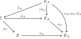
Recall thathφC,0(RA)iis the kernel of the isogenyψCA,0on EC,0, see Figure 7.

Therefore, we can apply Corollary 4.8, and soψ_C0 is an endomorphism onEAC,0,

where kerψ_C0 =ψC

A,0(kerφ0C).

EC,0 EAC,0

ψC A,0

φ0C

ψ0 C

ψC A,00

Fig. 7:φ0C fixing the kernel ofψCA,0

LetψC_A,₀0be the isogeny onEC,0with kernelφ0C(kerψ C

A,0). Since gcd(k, N1) =

1, the following equation holds:ψC_A,₀0◦φ0_C ∼=ψ_C0 ◦ψC_A,₀.

It remains to be shown thatEAC,0∼=EAC,1,2, that is, the codomain of ψA,C0

0 is isomorphic toEAC,0. Similar to above we find

kerψ_A,C₀0 =φ0_C(kerψC_A,₀)

=φC,2◦φC,1◦φbC,0(hφC,0(RA)i)

=φC,2◦φC,1(h[degφC,0]·RAi) = [degφC,0]·ker(ψA,C1,2)

= ker(ψ_A,C₁_,₂). Then,

EAC,1,2∼=ψA,C1,2(EC,1,2)∼=ψCA,0

0₍_E C,0) ∼

=ψ_A,C₁_,₂◦φ0_C(EC,0)∼=ψC0 ◦ψ C

A,0(EC,0)∼=EAC,0.

ThusEAC,0 andEAC,1,2 are isomorphic. Hence

ECA,0∼=EAC,0∼=EAC,1,2∼=ECA,1,2.

However,ψC,2is ak-isogeny betweenECA,1andECA,1,2. This impliesECA,1and

ECA,0arek-isogenous.

Ifkis small enough, then Lemma 5.6 will prove useful in the coming reduction. We note the similarity of Theorem 5.7 to Theorem 4.9, except that it allows us to extract a factor of up toN2

2 out of the runtime of Theorem 4.9.

(20)

1. a starting supersingular elliptic curve E(_Fp2) such that p=N₁N₂−1 for

coprime N1 andlogp-smooth N2,

2. the image curve of anN1-degree isogenyEA=φA(E)with kernelhRAi,

3. the action φA|E[N2], and

4. a triangular kernelker4φC of a cyclic Lk-degree endomorphismφC inFp2

such that:

(a) gcd(k, N1) = 1,

(b) L|(N2)2, and

(c) k < N1.

Then there exists a (classical) algorithm with worst case runtimeO˜(k3₎_which

decides whether RA∈EigN1(φC)or RA6∈EigN1(φC)with overwhelmingly high

probability. Further, if kis logp-smooth, then the runtime isO˜(√k).

We start by describing the algorithm referred to in the theorem, thereby showcasing its existence, and subsequently analyze its running time and success probability to prove the theorem. The probability of a false-positive (our algorithm sayingRA∈EigN1(φC) whenRA∈/EigN1(φC)), can be approximated using the

mixing properties of the isogeny graph.

Algorithm 5.8.

Input:E, p, N1, N2,{PA, QA}, EA, φA|E[N2],ker4φC= (K0, K1, K2), and a

nat-ural numberk=|K2|. Note: K2 is not actually needed, onlyk=|K2|. Output: True ifRA∈EigN1(φC), and False ifRA6∈EigN1(φC)

1. Use φA|E[N2] to computeφA(K0) andφA(K1).

2. Compute the isogeniesψC,0, andψC,1 with respective kernelshφA(K0)iand hφA(K1)i(see Figure 6).

3. For all k-isogenies from ECA,0, check if their codomain has j-invariant

j(ECA,1).

4. If one does, then return True, otherwise return False.

Proof. First, we discuss the success probability. If Algorithm 5.8 returns False, then r1A

is not an eigenvector with respect to φC by the contrapositive of Lemma 5.6. Suppose Algorithm 5.8 returns True. Notice that the total number of non-backtracking isogenies fromECA,0of degree k, if we write the factorization

k= Q

1≤i≤r qei

i , is

Y

1≤i≤r

(qi+ 1)qiei−1.

Also, we know that there are approximately ₁₂p isomorphism families of elliptic curves in an isogeny graph. From these two pieces of information we deduce that the probability that there is a cyclick-isogeny betweenECA,0 and ECA,1 is no

more than

12 p

Y

1≤i≤r

(21)

This probability is negligible sincek < N1≈ √

p. Therefore, under this assumption on k, if there is ak-isogeny fromECA,1 toEA, then the kernel subgroup is fixed byφC.

Next, we discuss the runtime. Step 1 and Step 2 are efficient inpsinceN2 is

logp-smooth. The analysis of verifying when ECA,1 andEA arek-isogenous is identical to the proof of Theorem 4.9. Thus, the worst case is whenk is prime, with runtimeO(k3_).

It follows from this theorem that ifkis small enough, then it will be feasible to test if an unknown kerφAis fixed by an endomorphismφC or not. Algorithm 5.8 will be a subroutine in our main reduction (Theorem 5.11). That reduction will assume an oracle which outputs triangular kernels of endomorphisms, and then use Algorithm 5.8 with each of those endomorphisms. In Section 7.3 we demonstrate that the SIKE/SIDH starting curve likely does not have an endomorphism which satisfy the conditions of Theorem 5.7.

5.2 Main Theorem

In this section, we present the first main result of the paper, Theorem 5.11. We prove this result by describing Algorithm 5.12 and analyzing its runtime. We start by presenting Oracle 5.9, which we will use in our reduction.

As mentioned previously, it is useful for the oracle to output a triangular kernel, instead of the kernel, to avoid unnecessary extension fields, see Remark 5.2. Since we are no longer discussing a singleLk-isogeny, withk≤N1, but potentially

multiple from repeated calls to an oracle, we instead use K ≤ N1 to denote

the upper bound on all such k. We also introduce the variable ρ to quantify the amount of information each endomorphism provides. The closerρis to 1/2, the closer the endomorphism is to providing a full bit of information on Alice’s private key (by the definition ofH(ρ)).

Oracle 5.9.

Input:E,p,N2, a setS⊆E[N1], an integerK≤N1, andρ∈(0,1/2] satisfying

ρ=ω(1/poly(λ)).

Output:The ker4φC = (K0, K1, K2) of a cyclic endomorphismφC such that

the following constraints hold: 1. |K2| ≤K,

2. gcd(|K2|, N1) = 1,

3. |S∩EigN1(φC)| ≤(1−ρ)· |S|, and

4. |S\EigN1(φC)| ≤(1−ρ)· |S|,

or it returns⊥if no endomorphism satisfying these constraints exists.

With the following definition, we give a name to the endomorphisms output by Oracle 5.9.

Definition 5.10. We call an endomorphism that satisfies the conditions of

(22)

The next theorem gives our main reduction. In essence, it states that each endomorphismφC returned by Oracle 5.9 can be used to gain information about Alice’s private keyrA. More specifically, it is possible to use Algorithm 5.8 to decide whether or notRA is in the eigenspace of each endomorphismφC.

1. a starting supersingular elliptic curve E(_Fp2) such that p=N1N2−1 for

coprime N1 andlogp-smooth N2,

2. the image of anN1-degree isogenyEA=φA(E),

3. the action φA|_E_[_N_2], and

4. access to Oracle 5.9,O, such that for an overwhelming fraction of sets S,O

will succeed for a non-negligible fraction ofK∈ {0, . . . , N1}andρ∈

h

1

f(λ), 1 2

i

, wheref is some fixed polynomial.

Then there exists a (classical) algorithm which outputsrA, wherekerφA=hRAi,

with non-negligible probability, makes m = O logN1

−log(1−ρ)

queries to O, and

runs in worst-case time O K˜ 3·m. Further, if the endomorphisms all have

logp-smooth degree, then the runtime isO˜√K·m.

We now present the algorithm that is referred to in Theorem 5.11. At a high level, Algorithm 5.12 iteratively reduces the size of the search space, which is denotedSi at theithiteration, for Alice’s private point. Step 5 is not required to prove the runtimes as stated in Theorem 5.11, however, we include it to highlight operational improvements that can be made.

Algorithm 5.12.

Input: E, p, N1, N2,{PA, QA}, EA, φA|_E_[_N_2], the polynomial f, and access to Oracle 5.9 denotedO.

Output:rAor ⊥.

1. LetS0={PA+ [r]·QA|0≤r < N1},andi= 0.

2. Setρ= 1/f(λ). 3. SetK=N1.

4. CallOwith (E, p, Si, N2, K, ρ) :

IfO outputs⊥, then return⊥.

Else, obtain φC from O(satisfying the conditions 1 to 4 from Oracle 5.9). 5. WhileOoutputs a solution:

HalveK and call O. LetK be the last value whereOdid not output⊥. Whileρ≤1/2, andOoutputs a solution:

Double ρand call O.

Letρbe the last value for whichOdid not output⊥.

Let (K0, K1, K2) be the output ofO called with (E, p, Si, N2, K, ρ).

(23)

7. Use the Algorithm 5.8 with input E, p, N1, N2, {PA, QA}, EA,φA|E[N2],

(K0, K1, K2), andkto determine whether RA∈X orRA∈Y.

8. IfRA∈X, then letSi+1=X, otherwise ifRA∈Y, then letSi+1=Y.

9. Incrementiand repeat Steps 2 to 8 until|Si| ≤f(λ).

10. For each pointR∈Si, compute the isogeny with kernelhRi, and returnRif the image curve is isomorphic toEA.

We now analyze Algorithm 5.12, thereby proving Theorem 5.11.

Proof. (Theorem 5.11) The proof will consist in analyzing the success probability and runtime of Algorithm 5.12. In particular, we will now show that in the setting of Theorem 5.11, Algorithm 5.12 runs in timeK3_poly(_λ_).

Letσ1be the fraction of setsS ⊆E[N1] for which there exists a non-negligible

amount ofK≤N1 andρ≤1/2 for whichOwill succeed. By hypothesisσ1 is

exponentially close to 1. Hence, with probabilityσ1, the reduction makes it to

Step 8 instead of outputting⊥.

Note that at the end of Step 7,|Si+1| ≤(1−ρ)|Si|for alli. Let C= poly(λ) andm=llogN1−logC

−log(1−ρ)

m . Then

log|Sm| ≤log ((1−ρ)mN1)

=mlog(1−ρ) + logN1 ≈logN1−logC

−log(1−ρ) log(1−ρ) + logN1

= logC.

This implies that to ensure|Sm| ≤(1−ρ)mN1 has polynomial size,O(m) calls

to O are required. Therefore, we expect there to be at least O(log(λ)) many iterations of Steps 2 to 8.

Step 5 performs two binary searches usingO. The search for the minimumK takes logN1 calls, and the search for the maximumρtakes log(poly(λ)) calls, for

a total of poly(λ) calls. By the statement of Theorem 5.7, Step 7 will terminate with high probability, sayσ2, in worst case time ˜O(K3). Therefore, since Steps 2

to 8 happensO(logλ) many times, Algorithm 5.12 terminates in worst-case time K3poly(λ) log(λ), and succeeds with probability (σ1σ2)O(log(λ))= 1−negl(λ).

We will further discuss the relationship betweenρandKin Section 9.2.

6 Quadratic Forms and Endomorphism Rings

If we know the structure of End(E), then we can efficiently reduce Oracle 5.9 to an oracle which finds solutions to a particular multivariate quadratic equation that satisfy certain algebraic conditions. In particular, once the endomorphism is described in terms of a basis, then finding an endomorphism of a particular degree amounts to finding a solution to a particular multivariate quadratic equation (see Section 6.1). Similarly, if we choose a basis for both End(E) andE[N1], then the

(24)

6.1 Quadratic Forms from Degrees of Endomorphisms

So far we have been describing endomorphisms by giving their kernels. Since an endomorphism is well-defined up to isomorphism by its kernel, knowing its kernel, or even better a triangular kernel, makes it is easy to calculate the endomorphism using V´elu’s formulas.

It is well known that the endomorphism ring of an elliptic curveE has the structure of a 4-dimensional_Z-module. In other words, there exist endomorphisms b1, b2, b3, b4 ofEsuch that

{[w]·b1+ [x]·b2+ [y]·b3+ [z]·b4|w, x, y, z ∈Z}

describes the set of endomorphisms inE. We use the phrase knowing the en-domorphism ring of an elliptic curve, to mean that we know an explicit basis

{b1, b2, b3, b4}of End(E).

One advantage of a basis representation is that there is a simple formula for computing the degree of a general endomorphism in terms of the respective traces and degrees of the endomorphisms in the basis. Another advantage, which we will see in Section 6.2, is that the description of an endomorphism in terms of a well-known basis makes it easy to explicitly find the eigenspace of that endomorphism.

In Proposition 6.3 we will show how to turn a description of an endomorphism in terms of a basis of End(E) into the triangular kernel description, so that the results of Section 5 can be utilized. We will do this using the following lemma, which shows how to find the action of an endomorphism on a torsion subgroup from its basis coefficients.

Lemma 6.1. Suppose End(E) =hb1, b2, b3, b4iand N is a natural number. For

integer variables (w, x, y, z), the action of any endomorphism

[w]·b1+ [x]·b2+ [y]·b3+ [z]·b4

onE[N] can be written as a2×2-matrixM(w, x, y, z)whose entries are linear in the four variables. In the worst case, this can be done inO˜(N3₎_{time and in}

the best caseΩ(log2p) time (whenN islogp-smooth).

Proof. We prove Lemma 6.1 by describing an algorithm that returns the required output and analyzing its runtime. Consider the factorization ofN = Q

1≤i≤r qei

i .

Algorithm 6.2.

Input: E, a basis{b1, b2, b3, b4}of End(E), integer variables (w, x, y, z),N,and

optionally a basis{P, Q} forE[N].

Output: A 2×2-matrixM(w, x, y, z) whose entries are linear in the four variables

and a basis{P, Q} forE[N] if it was not provided.

1. IfP, Q is not given, find a basis{P, Q}ofE[N]⊂E(Fp2).

2. Calculate bi(P) and bi(Q) for i = 1, . . . ,4. Solving the discrete logarithm for these values, in terms ofP andQ, gives bi|E[N] which we can write as a

matrixMi.

(25)

4. Output P, Q, M.

The most difficult part of Algorithm 6.2 is constructing the field extension in Step 1. Once the extension is constructed, the arithmetic in that extension is efficient inN andp. Recall that Step 1 has runtime ˜O(N3_{) in the case where}_E_[_N_]

is not defined overFp2, as seen in the proof of Theorem 4.9. The best-case scenario

for constructing the basis in Step 1 takesΩ(log2p) whenN is logp-smooth or theN-torsion is defined over a small field extension (see Theorem 4.9).

Step 2 has runtimeO P

1≤i≤r

ei(logN+√qi)[19], which is always less than

the runtime in Step 1.

Now, we will use Lemma 6.1 in Proposition 6.3 to transform endomorphisms (in terms of their basis) into a triangular kernel. This will allow us to apply

Theorem 5.11 with the basis representation.

More specifically, in Proposition 6.3 we will find a triangular kernel (K0, K1, K2),

whereφC =φbC,0◦φC,2◦φC,1. To do this we first fix the orders of K0, K1, K2

to be numbers that satisfy the conditions of a triangular kernel. Additionally, gcd(|K2|, N1) = 1. We can use Lemma 6.1 and the following facts to find

(K0, K1, K2):

• kerφC,0= kerMc, where Mcdescribes the action ofφbC onE[|K0|], • kerφC,1= kerM, where M describes the action ofφC onE[|K1|], and • kerφC,2=φC,1(kerMk),whereMkdescribes the action ofφConE[|K1| · |K2|].

Proposition 6.3. Suppose we are given

1. a starting supersingular elliptic curve E(_Fp2) such that p=N₁N₂−1 for

coprime, positive integers N1 andN2, such thatN2 islogp-smooth,

2. a basis{b1, b2, b3, b4} of End(E), and

3. a cyclicLk-degree endomorphism

φC= [w0]·b1+ [x0]·b2+ [y0]·b3+ [z0]·b4

of E, whereL|(N2)2.

Then there exists an algorithm to find points generating the triangular kernel of φC with respect to N2 whose worst case runtime is O˜(k3). Further if k is

logp-smooth, then the runtime is O˜(√k).

Proof. We prove Proposition 6.3 by describing the necessary steps in the algorithm and analyzing their runtime.

1. Write degφC=Lk withLmaximal such thatL|(N2)2.

2. Let L0= min(L, N2). We will find a triangular kernel (K0, K1, K2),where |K1|=L0,|K0|=L/L0,and|K2|=k.

3. First we solve for K0. Fix a basis {P0, Q0} =

nh N2

|K0|

i PB,

h N2

|K0|

i QB

(26)

4. We will use the fact that kerφC,0 = kerMc, whereMcdescribes the action ofφbonE[|K0|]. That is, run Algorithm 6.2 with input{bb1, . . . ,bb4}, integer

variables (w, x, y, z),|K0|and the basis{P0, Q0} forE[|K0|]. Let the output

be the matrixMc. 5. Find some vector α0

β0

which generates the kernel ofMc(w0, x0, y0, z0). Set

K0= [α0]·P0+ [β0]·Q0.

6. We now find the kernel point K1 in a similar process. Fix a basis{P1, Q1}=

nh N2

|K1|

i PB,

h N2

|K1|

i QB

o

ofE[|K1|].

7. We will use the fact that kerφC,1= kerM, whereM describes the action of

φC onE[|K1|]. That is, run Algorithm 6.2 with input{b1, . . . , b4}, integer

variables (w, x, y, z),L0 and basis{P1, Q1} forE[|K1|]. Let the output be

the matrixM. 8. Find some vector α1

β1

which generates the kernel ofM(w0, x0, y0, z0). Set

K1= [α1]·P1+ [β1]·Q1.

9. Lastly we describe how to find the kernel point K2. We perform a similar

process to the last two kernel points, except we need to push the point through an isogeny (see Definition 5.1).

10. Run Algorithm 6.2 with{b1, . . . , b4},integer variables (w, x, y, z), andk. Let

the output be the matrixMk and the basis{Pk, Qk}forE[k]⊂E(Fp2).

11. Find some vectorαk

βk

which generates the kernel ofMk(w0, x0, y0, z0).

12. LetφC,1be the isogeny fromEwith kernelhK1i, and setK2=φ1([αk]·Pk+ [βk]·Qk).

13. ReturnK0, K1, K2.

Steps 4 and 7 run in timeO(logp), since N2 is logp-smooth and E[N2]⊂

E(Fp2). By Lemma 6.1, Step 10 will run in worst case time ˜O(k3) and best case

time ˜O(√k) whenk is logp-smooth (assumingkdoes not divideN2, in which

case it is even better).

Remark 6.4. The converse of Proposition 6.3 is true as well, in the sense that

there exists an algorithm which outputs coefficients (w, x, y, z) upon input of a triangular kernel forφC with respect toN2, and it has the same runtime. We do

not state this converse algorithm, as will we not use it.

Proposition 6.3 will allow us to convert Oracle 5.9 (which returns an endomor-phism in terms of a triangular kernel) to an oracle that returns the coefficients of an endomorphism in terms of a basis. The advantage of this becomes apparent when we look at the explicit description of the degree and eigenspaces of an endomorphism represented in terms of a basis.

More specifically, associated to any basis of the endomorphism ring is a 4-variable quadratic form which represents the degrees of the endomorphisms.

Lemma 6.5. IfφC= [w]·b1+ [x]·b2+ [y]·b3+ [z]·b4 is any endomorphism

(27)

of φC is given by the following quadratic form:

q(w, x, y, z) =φC◦φbC= [w2degb1+x2degb2+y2degb3+z2degb4

+wxTr(b1bb2) +wyTr(b1bb3) +wzTr(b1bb4) +xyTr(b2bb3)

+xzTr(b2bb4) +yzTr(b3bb4)].

From Proposition 6.3 and Lemma 6.5 we see that an oracle which outputs solutions to certain quadratic forms may be used instead of an oracle that outputs triangular kernels. This new oracle will be presented at the end of Section 6.2 (see Oracle 6.11). Next we explore what the eigenspace conditions of Oracle 5.9

become if we use this basis description of endomorphisms.

6.2 Quadratic Forms from Eigenspaces of Endomorphisms

In the last subsection we showed that, if End(E) is known, then instead of representing endomorphisms by triangular kernels, we can represent them in terms of a basis of End(E). We saw that this basis representation allows for a simple description of the degree and the action of the endomorphism on the set of Alice’s possible private points.

In this subsection, we explore when the eigenspace requirements (Conditions 3 and 4) of Oracle 5.9 are satisfied, assuming the endomorphism is described in terms of a basis. We do this by first analyzing the eigenspace of a random matrix onE[N1]. We simplify our calculations by assuming thatN1 is a prime power,

although a similar analysis should work ifN1 is any logp-smooth number.

The following notation will be useful in the main theorem of this subsection.

Notation 6.6. Let` andebe fixed positive integers. Normally, in SIDH and

in SIKE, `e_{= 2}a _or_`e_{= 3}b_{. Let}hα β γ δ i

denote a matrix with entries in _Z/`e

Z.

Given an eigenvector [1

r] of this matrix and a fixed small prime`, we use the following notation in the remainder of this document:

• ν denotes the largest natural number such that`ν _|_β _and_`ν _|_δ₋_α_.

• β0, 0 are the numbers such thatβ=`νβ0 andδ−α=`ν0.

• ξis the largest natural number such that`ξ _|0₋₂_β0_r_and_ξ_≤e−ν

2 . • ζ=e−ν−ξ.

Remark 6.7. In Theorem 6.8 we will describe the `e_{-eigenspace of a matrix}

M. We will see in the proof of Theorem 6.8, that the definitions of ξandζ are independent of the choice of eigenvector [1

r] ofM. In other words,ξandζ are defined with respect toM and prime `.

Theorem 6.8 shows that if there is an eigenvector of a matrix and the associated ζ is small, then there are many eigenvectors.

Theorem 6.8. Suppose there is an eigenvector [1

r]of a matrix h_{α β}

γ δ i

(28)

• If`|β0, then [1

κ]is an eigenvector if and only if it has the form h ₁

r+c`ζ i

for somec∈_Z.

• If`_-β0, then[1

κ] is an eigenvector if and only if it has the form h ₁

r+c`ζ

i

or

h ₁

−r+0(β0)−1+c`ζ

i

for somec∈Z.

Proof. Note that [1

r] is an eigenvector of the matrix h

α β γ δ i

over _Z/`e

Z if and

only ifγ+ (δ−α)r−βr2_≡_{0 (mod}_`e_{), see Lemma A.1. Now, suppose} 1

r+x

is also an eigenvector. This implies

γ+ (δ−α)r−βr2≡0 (mod`e) and

γ+ (δ−α)(r+x)−β(r+x)2≡0 (mod`e). Subtracting these two equations shows that 1

r+x

is an eigenvector if and only ifxsatisfies:

(δ−α)x−β(2rx+x2)≡0 (mod`e). This is equivalent to

(δ−α−β(2r+x))x≡0 (mod`e). (3) and also,

(0−β0(2r+x))x≡0 mod`e−ν. (4) Suppose ` | β0. Then ` - 0, and hence a vector of the form r+1x

is an eigenvector if and only if it has the formx≡0 (mod`e−v₎_._{This is equivalent to} saying 1

r+x

has the formh_r₊1_c`ζ

i

,sinceξ= 0. Suppose`-β0. Then Equation (4) is equivalent to

(0(β0)−1−(2r+x))x≡0 mod`e−ν. (5) Further supposex is a solution to Equation (5). One of the following two cases holds:

x≡ −2r+0(β0)−1 mod`ζand x≡0 mod`ξ,

or

x≡0 mod`ζ and

x≡ −2r+0(β0)−1 mod`ξ. Thus the eigenvector 1

r+x

must have the form given in the theorem.

Conversely, suppose that x = c`ζ_{. By the definition of} _ξ_{, we have that} x≡0≡ −2r+0β0−1 _mod_`ζ

.Thusxis a solution to Equation (5). Now suppose thatx=−2r+0β0−1₊_c`ζ_,_then_x_≡_{0 mod}_`ξ

.Thusxis a

solution to Equation (5).

Remark 6.9. Theorem 6.8 proves that for a matrix

(29)

2. the probability that a random point of order `e _{is an eigenvector is}_`−ζ _or

1 2`

−ζ _{(depending on if}_`_|_β0_).

Given a basis{b0, b1, b2, b3}for an endomorphism ring, Lemma 6.1 shows that

the action of the set of endomorphisms

{[w]·b1+ [x]·b2+ [y]·b3+ [z]·b4|w, x, y, z ∈Z}

on E[`e_{] can be given a 2}_×_2-matrix _M₍_{w, x, y, z}_{) whose entries are linear in} the four variables. Thus, we are interested in the values (w0, x0, y0, z0) which

the matrix M(w0, x0, y0, z0) has many eigenvectors. In other words, we want

M(w0, x0, y0, z0) to have at least one eigenvector andζ to be small. We will now

replace Conditions 3 and 4 of Oracle 5.9 with more concrete conditions. This allows us to restate Theorem 5.11 with an oracle that has a more concrete output.

Remark 6.10. In order to use of Theorem 6.8 to derive the following

ora-cle/reduction, we requireN1=`e. For a more general statement simply replace

Conditions 4 and 5 in Oracle 6.11 with a condition that eigenspace ofφCseparates S(the space that potentially contains Alice’s private point) into two large subsets (as in Oracle 5.9).

Oracle 6.11.

Input:E, p, N2, a setS ⊆E[`e], a quadratic formq(w, x, y, z), a 2×2-matrix

M(w, x, y, z) acting onE[`e_{] whose entries are linear in the four variables, an} integer K≤`e, ands∈[0, e].

Output:Integers (w0, x0, y0, z0), with no common divisor, satisfying the equation

q(w0, x0, y0, z0) =Lk, such that the following constraints hold:

1. k≤K, 2. L|(N2)2,

3. gcd(k, `) = 1,

4. M(w0, x0, y0, z0) has at least one eigenvector, and

5. M(w0, x0, y0, z0) hasζ < s, (whereζ is defined with respect toM and`),

or⊥if no solution satisfying these constraints exists.

The next theorem is analogous to Theorem 5.11 and constitutes the second main result of this work. It states that endomorphisms associated to the outputs of Oracle 6.11 can be used to gain information about Alice’s private keyrA.

1. a starting supersingular elliptic curveE(_Fp2)such thatp=N₁N₂−1 forN₁

coprime to N2, whereN1=`eand N2 islogp-smooth,

2. bases{PA, QA} ofE[N1]and{PB, QB} of E[N2],

3. a basis{b1, b2, b3, b4} of End(E),

4. the image of anN1-degree isogenyEA=φA(E),