Thesis by
Adam Norman
In Partial Fulfillment of the Requirements for the Degree of
Doctor of Philosophy
California Institute of Technology Pasadena, California
2010
c
2010
Acknowledgments
I would like to begin by thanking my advisor, Professor Beverley McKeon. The past four years in her research group have been very enjoyable. I am grateful that Beverley gave me a certain amount of freedom to guide my own research, while at the same time always encouraging me to think more deeply and theoretically. My years in her group would not have been the same without the amazing research group that built up over time. I greatly appreciate the enthusiasm and thoughtful discussions with my various committee members: Tim Colonius, Mory Gharib, Fazle Hussain, Tony Leonard, and Dale Pullin. Special thanks go to Fazle for being on my committee even though it required travel.
This work was improved by the help of many other people. In particular I would like to thank Dr. Eric Kerrigan from Imperial College London for teaching me so much about control theory, and for spending time getting the motor controller working so well, which made some of this research possible. I would also like to thank Dr. Luca Maddalena for his input on my design, and Jeff LeHew for showing me how to build a power-boosting circuit.
I also appreciate the help of the aeroshop staff, particularly Ali for his precise workmanship on much of my design. The administrative staff was also great, always willing to help. I was also lucky to share an office with many great people.
I have benefited from the friendship of many people while at Caltech, though I must thank Geoff Ward in particular. We have enjoyed many games of ping-pong, tennis, and racquetball, along with many other activities outside of Caltech.
Thanks must also go to my flight instructor, Joe Areeda, who shared his passion of flying with me. He did not charge me nearly enough for flying lessons, and his response was that it did not matter because there was no other job with such a great view out the window. Though I have not had much time to fly since getting my pilot’s license, I often dream of being up in the sky when I am sitting at my desk.
The most important acknowledgments go to my family. My parents and brother have always believed in me, giving me the confidence to pursue my dreams. In addition, I appreciate the encouragement of my wife’s family, who are much more than just in-laws to me. Finally, this work simply would not have been possible without the love and support of my wife. While in California we have enjoyed many great adventures together, the most exciting being raising our wonderful son, who is 18 months old at the time of writing.
Abstract
Contents
Acknowledgments iv
Abstract v
1 Introduction 1
1.1 Motivation . . . 1
1.2 Background . . . 2
1.2.1 Flow Over a Smooth Sphere . . . 2
1.2.2 Effect of Static Changes to the Sphere Shape . . . 4
1.2.3 Active Manipulation of the Flow . . . 5
1.3 Thesis Outline . . . 6
2 Experimental Methods 7 2.1 Experimental Facility . . . 7
2.2 Model and Test Stand . . . 7
2.2.1 Coordinate System . . . 7
2.2.2 Rigid Stand . . . 9
2.2.3 Sphere Model . . . 10
2.2.4 Surface Actuation . . . 11
2.3 Actuation Method . . . 12
2.4 Measurement Techniques . . . 16
2.4.1 Time-Resolved Three-Component Force Measurements . . . 16
2.4.2 Particle Image Velocimetry . . . 16
2.4.3 Hot-film Anemometry . . . 17
2.5 Data Reduction . . . 17
2.5.1 Signal Conditioning . . . 17
2.5.2 Current Correction . . . 18
2.5.3 Analysis Routines . . . 18
3 Forces on a Smooth Sphere 20
3.1 Overview . . . 20
3.2 Fluctuating Forces . . . 20
3.3 Statistical Convergence . . . 21
3.4 Mean Force and Higher Moments . . . 25
3.5 Force Spectral Density . . . 27
3.6 Synchronous Velocity Field and Force Histories . . . 31
3.7 A Simple Force Model . . . 31
3.8 Discussion and Summary . . . 37
3.8.1 Structure of the Sphere Wake . . . 37
3.8.2 Sampling Time for Statistical Convergence . . . 38
4 The Effect of a Small Stationary Isolated Roughness Element 39 4.1 Overview . . . 39
4.2 Reynolds Number Dependence of the Mean Forces . . . 40
4.2.1 Influence of Streamwise Location of the Roughness Element . . . 41
4.2.2 Associated Near-Wake Structure . . . 42
4.2.3 Effect of Stud Size . . . 48
4.3 Spectral Density . . . 49
4.4 Moments . . . 52
4.5 Summary . . . 55
5 The Effect of Small-Amplitude Time-Dependent Changes to Surface Morphology 57 5.1 Overview . . . 57
5.2 Roughness Element Moving at Constant Speed . . . 57
5.2.1 Effect of Reynolds Number . . . 58
5.2.2 Flow Response Time . . . 61
5.2.3 Effect on Mean Flow . . . 63
5.2.4 Instantaneous Velocity Field . . . 63
5.2.5 Phase-Averaged Flow Field . . . 66
5.3 Shaped Trajectories . . . 73
5.3.1 Oscillating Roughness Element . . . 73
5.3.2 Velocity Profile Shaping . . . 73
5.3.3 Effect of a Step in Angular Frequency . . . 77
6 Conclusion 80
6.1 Summary and Major Findings . . . 80
6.2 Future Research . . . 81
A Effect of Sting Size at Subcritical Reynolds Numbers 83 A.1 Overview . . . 83
A.2 Introduction . . . 83
A.3 Experimental Setup . . . 84
A.4 Results . . . 87
A.4.1 Convergence . . . 87
A.4.2 Mean Wake . . . 89
A.4.3 Periodic Behavior . . . 91
List of Figures
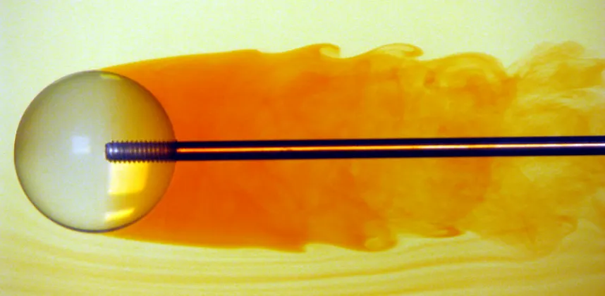
1.1 Dye visualization at a Reynolds number of 3.8×10³, showing the roll-up of the shear layer in the near wake. . . 2
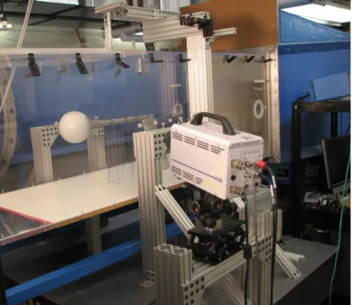
2.1 Sphere centered in test section, showing the support structure for the sting and the piano wires, along with the PIV camera and optical table. . . 8 2.2 (a) Coordinate system chosen with x as the streamwise direction. The streamwise angle from
the stagnation point isφ, with theksubscript indicating the streamwise angle to the stud. The drag coefficient is labeledCD. (b) Looking downstream: the lateral force coefficient vector is labeledC~L, and is composed ofCyyˆ+Czzˆ.θ is the lateral angle from they-axis toC~L. . . 9 2.3 (a) Model in 61cm by 61cm recirculating wind tunnel test section, with piano wires used to
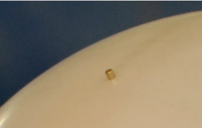
increase the natural frequency of the sphere-support system. (b) Inside of the sphere showing the motor, motor arm and magnet, and three-component force sensor attached to a stainless steel base. . . 10 2.4 Stud with a width and height ofk/D=0.01, held in place with a magnet that is inside of the
sphere. . . 11
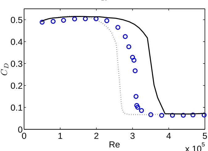
3.1 Variation of the coefficient of mean drag with Reynolds number: present data (o) compared with the results of Achenbach for a smooth (−) and slightly rough sphere (k/D=2.5×10−4,
....). . . . 21
3.2 Time trace of the lateral forces for (a) subcriticalRe=1.1×10⁵with∆tˆ=250 and (b) super-criticalRe=4.1×10⁵with∆tˆ=800. . . 22 3.3 Statistical convergence of dynamic force data: standard deviation of the moments as a function
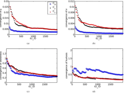
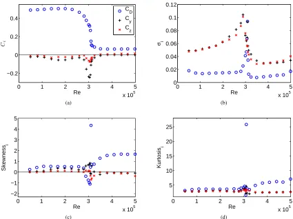
of averaging time, subcriticalRe=1.1×10⁵, . . . 23 3.4 As figure 3.3, supercriticalRe=4.1×10⁵. . . 24 3.5 Statistical summary of the force coefficients,Ci,: (a) mean (b) standard deviation (c) skewness
and (d) kurtosis. . . 25 3.6 Probability density for: subcritical Reynolds numbers (1) 1.1×10⁵, (2) 2.6×10⁵; criticalRe
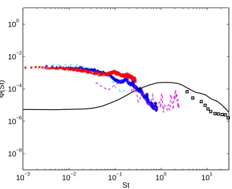
3.7 Normalized power spectral density of the subcritical lateral forces, compared with the lit-erature. The lateral force spectra were averaged. Present results, Re=8×10⁴ (+) and
Re=2.3×10⁵(x); Constantinescu & Squires (2004) (−−),Re=104; Yunet al.(2006) (−.−),
Re=104; Howeet al.(2001) model (–); Howe experiments (), 7×10³<Re<1.7×10⁴; Lauchle & Jones (1998) (♦), 7×10³<Re<3.5×10⁴;St−3(...). . . 28 3.8 Normalized power spectral density of subcritical drag force, compared with the literature.
Symbols as in figure 3.7. . . 29 3.9 Normalized power spectral density of supercritical lateral force, compared with the literature.
Re=3.8×10⁵(+);Re=5.0×10⁵(x); Willmarth & Enlow (1969) (−.−), 4.8×10⁵<Re<
1.7×10⁶; Constantinescu & Squires (2004) (−−),Re=1.1×10⁶. . . 29 3.10 Normalized power spectral density of supercritical drag force, compared with the literature.
Symbols as in figure 3.9. . . 30 3.11 Simultaneous PIV and force data forCy: (a) positive (b) zero and (c) negative.Cx(-·-);Cy(–);
Cz(- -). . . 32 3.12 Schematic of a two-dimensional harmonic oscillator, with the restoring force being
propor-tional to the distance from the origin. . . 33 3.13 Probability density function of the side force,Cy, compared with measurements atRe=1×10⁵. 35 3.14 Power spectral density of the side force,Cy, compared with measurements atRe=1×10⁵. . . 35 3.15 Comparison of model results and measured data and the literature. . . 36
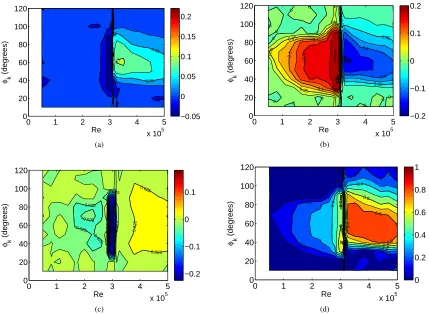
4.1 Mean force coefficients (Ci, whereirepresents the drag or one of the lateral force components) as a function ofRewithout a stud (a) and with a stud placed atθk=0◦,φk=70◦with diameter (b) 0.01D, (c) 0.02D, and (d) 0.04D. . . 40 4.2 Contour plots showing the effect of the stud’s streamwise angle,φk, andRefor a 1% stud: (a)
∆CD, (b)∆Cy, (c)∆Cz, and (d)|∆Cy/CD|. . . 41 4.3 70◦cut:∆CD(o);∆Cy(+);∆Cz(×);|∆Cy/CD|(O). . . 42 4.4 Mean velocity field and Reynolds stresses at a subcriticalReof 2.0×10⁵for (left) the smooth
sphere and (right) with a 0.01Dstud placed atφ=60◦(shown in red) in the plane of the image (θk=0◦). Top to bottom:u0u0/U∞2,v
0v0/U2
∞, andu
0v0/U2
∞. . . 43
4.5 Mean velocity field and Reynolds stresses at a supercriticalReof 4.1×10⁵for (left) the smooth sphere and (right) with a 0.01Dstud placed atφ=60◦(shown in red) in the plane of the image (θk=0◦). Top to bottom:u0u0/U∞2,v0v0/U∞2, andu0v0/U∞2. . . 45 4.6 The stationary stud locally delays separation in the subcritical regime, likely leading to the
4.9 SubcriticalRe of 8.0×10⁴ showing the normalized spectral density of the dynamic forces without a stud (a) and with a stud placed atθk=0◦,φk=70◦withk=(b) 0.01D, (c) 0.02D, and (d) 0.04D. . . 49 4.10 SubcriticalRe of 2.0×10⁵ showing the normalized spectral density of the dynamic forces
without a stud (a) and with a stud placed atθk=0◦,φk=70◦withk=(b) 0.01D, (c) 0.02D, and (d) 0.04D. . . 50 4.11 SupercriticalReof 4.4×10⁵showing the normalized spectral density of the dynamic forces
without a stud (a) and with a stud placed atθk=0◦,φk=70◦withk=(b) 0.01D, (c) 0.02D, and (d) 0.04D. . . 51 4.12 Standard deviation of the force coefficients as a function ofRewithout a stud (a) and with a
stud placed atθk=0◦,φk=70◦withk=(b) 0.01D, (c) 0.02D, and (d) 0.04D. . . 52 4.13 Probability density for: subcritical Reynolds numbers (1) 1.1×10⁵, (2) 2.6×10⁵; criticalRe
(3) 3.07×10⁵, (4) 3.09×10⁵, (5) 3.11×10⁵; and supercriticalRe(6) 4.1×10⁵. (a) no stud, (b) 0.01Dstud. . . 53 4.14 Skewness of the force coefficients as a function ofRewithout a stud (a) and with a stud placed
atθk=0◦,φk=70◦withk=(b) 0.01D, (c) 0.02D, and (d) 0.04D. . . 54 4.15 Kurtosis of the force coefficients as a function ofRewithout a stud (a) and with a stud placed
atθk=0◦,φk=70◦withk=(b) 0.01D, (c) 0.02D, and (d) 0.04D. . . 55
5.1 Static forces and a comparison with the smooth (−) sphere results from Achenbach (1974a): (a) smooth sphere results and (b) the same sphere with a 0.01Dstud placed atφk=60◦. . . 58 5.2 Time trace of the lateral force coefficients forRe=5×10⁴, showing that the dynamic stud
completely changes the force characteristics. The mean of the lateral force magnitude of the moving stud is up to seven times larger than that of the stationary stud. . . 59 5.3 MeanCLand phase (θ−θk) (in stud reference frame) vs. dimensionless angular frequency.
Re=0.5×10⁵(M);Re=0.8×10⁵(B);Re=1.1×10⁵(O);Re=2.0×10⁵(C);Re=3.1×10⁵ (o);Re=4.1×10⁵(). . . 60 5.4 (a) Uncalibrated hot-film voltage: lower voltage indicates greater heat transfer. Results are
forRe=5.0×10⁴and are averaged over 100 revolutions, as a function of the stud angle, in order to suppress voltage oscillations caused by vortex shedding. (b) Normalized with respect to time since the stud passed. No stud mean (-);ω∗=0.15 (); 0.34 (♦); 0.52 (M); 0.70 (B); 0.89 (O). . . 61 5.5 Mean velocity field and mean Reynolds shear stress for (left to right then top to bottom): no
5.6 Time trace of the forces along with four instantaneous velocity fields equally spaced over one stud revolution (indicated by vertical line on force history), with the stud moving atω∗=0.15. The vector field is in the x-y plane, and the forces are marked asCx(-·-);Cy(–);Cz(- -). . . . 64 5.7 Same as figure 5.6, except withω∗=0.52. . . 65 5.8 Same as figure 5.6, except withω∗=0.89. . . 67 5.9 Phase averaged velocity fields with 0.6U∞ subtracted off, with roughness element moving at
ω∗=0.89. Grayscale shading indicates value of dimensionless vorticity. The stud is at 65◦ in the top image and shows a negative vortex on the top right, and a positive vortex forming behind the sphere. In the bottom image the stud is at 100◦and the positive vortex is now fully formed. . . 68 5.10 Three-dimensional phase-averaged flow field, with roughness element moving atω∗=0.89.
Azimuthal vorticity contours are−3 (dark gray) and+3 (light gray). Radial velocity contours are−0.2 (blue) and+0.4 (red). The lateral force vector is attached to the front of the sphere. . 68 5.11 Angled views showing the radial component of the phase-averaged wake, with ω∗=0.15.
Contours are of the normalized radial velocity:−0.2,−0.1, 0.1, 0.2, 0.3, 0.4. . . 69 5.12 Same as in figure 5.11, withω∗=0.34. . . 70 5.13 Same as in figure 5.11, withω∗=0.52. . . 70 5.14 Same as in figure 5.11, with ω∗=0.70. Note the high speed positive velocity fluid, with
negativeUrfluid on either side, indicating counter-rotating vortices in the shape of a helix. . . 71 5.15 Same as in figure 5.11, withω∗=0.89. . . 71 5.16 Schematic simplification of a spanwise cut of the near wake, showing the progression of the
counter-rotating vortices as the region of influence of the stud increases: (a) the stationary stud produces vortices which push each other toward the center, (b) vortices move away from each other and (c) meet on the opposite side, now pushing each other away from the center. . . 72 5.17 Mean lateral force (Cy), with stud oscillating aboutθ =0◦, with amplitude:±40◦(C);±60◦
(B);±80◦(M).CxandCzwere not notably changed. . . 74 5.18 Shaped trajectories, with a step up in angular frequency atθstep, and a step back down at
θ=0◦:ω∗=0.17-0.55(x); 0.34-0.55(+). . . 74 5.19 Shaped trajectory corresponding to a step fromω∗=0.17 to 0.55 at 90◦. (a) The angular
coordinate is the stud position, with the stud moving counter-clockwise: Phase-averaged force (...);ω∗/2 (x). (b) MeanCL and phase (θ−θk) vs. constant frequencyω∗ results forRe= 0.5×10⁵(M), compared with the current trajectory. . . . 76 5.20 Three mean step responses, each averaged over 120 periods, with the error bars indicating±σ. 77
A.2 Convergence of the streamwise velocity (1) outside wake, (2) behind sphere, (3) near maxu0u0, and (4) downstream in wake, forD=0.016m andχ=0.50, with position indicated by (x/D,y/D) 86 A.3 Convergence of the maximum Reynolds shear stress in the wake,u0v0
max/U∞2. See table A.1
for symbols . . . 86 A.4 Consecutive averages over ˆt=50 showing large scale movement of the wake forχ=0.09, with
color indicating nondimensional velocity magnitude, (a) 100<tˆ<150, (b) 150<tˆ<200, and (c) 200<tˆ<250. . . 88 A.5 Mean velocity field overlaid with the mean Reynolds shear stressesu0v0/U∞2(a),(b)χ=0.25:
left has higher free stream turbulence (c),(d)χ=0.50: right sphere has low amplitude vibrations. 89 A.6 Shape of the mean wake forD=0.016m: (a) paths of maximum (top), minimum (bottom),
and constantU∞/2 (center) velocity magnitude. (b) Velocity magnitude along the maximum and minimum paths. . . 90 A.7 Paths of constantU∞/2 for each sphere size, showing influence of free stream turbulence and
vibrations. . . 91 A.8 Mean Reynolds stresses forχ=0.50,D=0.016m (a)u0u0, (b)v0v0. . . 91 A.9 Maximum of mean Reynolds stresses as a function ofχ, with error bars based on convergence.
Computational results from Yunet al.(2006) shown for comparison . . . 92 A.10 Magnitude of frequency spectrum peak (streamwise on the left and radial on the right) as a
function of position, normalized by the maximum value for each image, where the maximum peak in (c) is 65% as strong as in (a), and the maximum peak in (d) is 58% as strong as in (b). (a),(b)χ=0.50,St=1.085 (c),(d)χ=0.80,St=1.081. . . 93 A.11 (a),(c) Representative frequency spectrum of u-velocity and (b),(d) vibration frequency of
Nomenclature
ˆ
t Dimensionless time=tU∞/D
µ Dynamic viscosity
ω∗ Dimensionless angular frequency of stud=θ˙kD/U∞ φ Streamwise angle
ρ Fluid density θ Spanwise angle
~
CL Lateral force coefficient=Cyyˆ+Czzˆ
CD Drag coefficient=FD/(12ρU∞2π
D2 4)
Ci Force coefficient=Fi/(12ρU∞2π
D2
4), fori=x,y, orz
D Sphere diameter
f Frequency
k Characteristic roughness scale
Chapter 1
Introduction
1.1
Motivation
The research detailed in this thesis is motivated by the broad goal of understanding the effect of morphing surfaces on wall-bounded flows, with the aim of improving performance and efficiency for a wide range of technologies, as well as utilizing these surfaces to gain insight into the fundamental physical mechanisms that govern the behavior of the flow.
A morphing surface is different from traditional control surfaces, such as flaps on an aircraft, in that there is a continuous surface (a “skin”). The interest is in exciting and utilizing flow instabilities to coerce the flow to perform as desired, with minimal energy input. This is accomplished by making small amplitude, targeted changes to the surface, rather than large mechanical changes to the overall shape.
Because true morphing surfaces with a quick response time are not currently readily available, an exper-imental apparatus was developed which mimics some of the desired features. In order to demonstrate the potential of a morphing surface, a sphere was chosen as the base geometry, because it is well known that the flow is extremely sensitive to small changes in the surface condition. Instead of examining the effect of a true morphing skin, small amplitude changes to the surface were produced by moving a small isolated roughness element (a “stud”) along the sphere surface at a fixed streamwise angle. Because the flow is so sensitive to the surface finish, the stud was held in place by a small magnet located inside the hollow sphere, which was itself moved with the use of a small motor, removing the need to have slots or other discontinuities.
The flow regime examined in this study was that of flow over a sphere in which there is a large turbu-lent wake, with flow separation occurring near the equator. This “bluff body” flow is characterized by two instabilities, that of the wake and that of the free shear layer. Many objects in daily use are bluff, from cars to sports balls. Understanding why the flow separates, and how it can be enticed to remain attached, allows for the possibility of making more-efficient and better-performing devices. In addition, the dynamics of the separation share some similarities with stalled airfoils, as will be discussed in chapter 5.
mea-Figure 1.1: Dye visualization at a Reynolds number of 3.8×10³, showing the roll-up of the shear layer in the near wake.
surements when needed to interpret the force measurements. As will be shown, a single moving roughness element has a profound effect on the flow, dramatically altering the separation point over the entire sphere, and completely changing the dynamics of the wake. In addition, the response of the flow to the prescribed disturbance provided a better understanding of sphere flow in general.
This is a first step toward understanding the effect of a dynamic surface on the flow field and forces, and paves the way for future studies which will utilize true morphing surfaces. In addition, it is demonstrated that the new experimental apparatus is an excellent testbed for examining the effectiveness of morphing surfaces.
1.2
Background
The flow field around a sphere is very rich (see, e.g. figure 1.1), beckoning theorists, numerical modelers, and experimentalists alike. Here is given a brief overview of the literature that is relevant to the current study.
1.2.1
Flow Over a Smooth Sphere
the ubiquity of spheres in sports.
For the Reynolds numbers of this study, there are three flow regimes of interest. In the subcritical regime, laminar boundary layer separation occurs at about 80◦, producing a large mean drag coefficient that is nearly independent of Reynolds number. Following this is the critical regime, which is associated with the separation location moving from about 80◦to 120◦, causing a rapid drop in the drag coefficient (the “drag crisis”), and ending at the lowest drag state, the “critical Reynolds number”. In this regime the global flow is highly dependent on the condition of the boundary layer and in particular the transition process. In the supercritical regime, a separation bubble which decreases in size as the Reynolds number is increased has been identified using oil film visualization (Taneda, 1978; Suryanarayana & Prabhu, 2000). Achenbach (1972) did not detect the separation bubble in the supercritical regime when measuring the shear stress, though the previously cited studies and the similarities to cylinder flow (Roshko, 1961) suggest that it is present and contributes to producing the low drag state. At higher Reynolds numbers (beyond the scope of this study), the drag begins to increase again, transitioning to the transcritical regime, which begins when the point of boundary layer transition begins to move upstream (Achenbach, 1972).
There is conflicting evidence concerning the mean lateral force in the supercritical regime. Taneda (1978) observed a mean wake offset, corresponding to a side force, in early experiments. The observation that the direction of this offset could be manipulated using a small stud positioned on the sphere surface suggests that this could be the result of an initial asymmetry in the experiment. In simulations of sphere flow, the investigations of Constantinescu & Squires (2004) also showed a mean supercritical side force, although the authors noted this may be a result of the relatively short simulations rather than a physical result.
The fluctuating, three-component force distribution acting on the sphere reflects the instabilities and struc-ture of the wake. For sphere Reynolds numbers above approximately 800 and below the critical Reynolds number,Recrit =O(105), frequencies corresponding to both a small-scale shear layer instability and a larger wake instability dominate the force spectrum, while below this lower limit only the larger scale is observed (Sakamoto & Haniu, 1990; Kim & Durbin, 1988; Baki´c & Peri´c, 2005; Achenbach, 1974b). With increasing Reynolds number the Strouhal number (St=f D/U∞, where f is the frequency) of the shear instability
in-creases asRen(Kim & Durbin, 1988), with 0.5≤n<1 for 103<ReD<105, while the large-scale Strouhal number remains approximately equal to 0.2, typical of vortex shedding. The wake instability has been de-scribed as both a helical instability (Chomazet al., 2006) and as vortex shedding in a randomly rotating azimuthal plane (Sakamoto & Haniu, 1990). In the subcritical regime, computational studies (Yunet al., 2006; Constantinescu & Squires, 2004) have also found evidence of low frequency oscillations of the wake, below that of the large-scale vortex shedding frequency.
Though the mean drag force has been measured by many researchers, the literature concerning the dy-namic forces on a sphere is sparse. In the subcritical regime, Lauchle & Jones (1998) indirectly measured the forces on a suspended sphere using an accelerometer, obtaining the decay of the frequency spectrum for
fre-quency spectrum and the mean squared lift for the case of a rough sphere. The subcritical Reynolds number range has been examined computationally by Yunet al.(2006) with large eddy simulation (LES), while both the subcritical and supercritical regimes have been investigated by Constantinescu & Squires (2004) using detached eddy simulation (DES). The phenomenological model for subcriticalRedeveloped by Howeet al.
(2001) by considering the spectra developed by the shedding of randomly oriented vortex rings appears to give reasonable agreement with the trends in the existing literature for highSt.
The combination of axisymmetry, extreme sensitivity of the flow to boundary conditions, and the long sampling times required to obtain converged statistics make this a challenging flow to investigate either ex-perimentally or numerically, especially in comparison to the nominally two-dimensional flow over a cylinder. In particular, obtaining the three-dimensional velocity field required to fully capture the sphere wake remains challenging in experiments, while the resolution requirements imposed by a very thin (possibly transitioning) boundary layer and a broad wake, combined with the low frequency content, are numerically exacting.
1.2.2
Effect of Static Changes to the Sphere Shape
Though the effect of distributed surface roughness on the mean drag force experienced by a fixed sphere in uniform flow has been examined in detail (e.g., Achenbach, 1974a; Choiet al., 2006), there are few studies that consider asymmetric roughness distribution or isolated roughness elements. In the presence of distributed roughness the boundary layer at all azimuthal locations transitions to a turbulent state at a lower Reynolds number than it does for the smooth sphere, reducing the critical Reynolds number at which the flow changes from the high drag subcritical regime to the lower drag supercritical regime. This phenomenon is used as a control technique in the familiar example of the dimpled surface of golf balls, designed to maximize the velocity range during which the ball experiences the low drag regime. Similar drag curves have been observed by using a two-dimensional trip wire (Maxworthy, 1969). For a rough sphere beyond the critical regime, the drag increases well beyond smooth sphere levels (Achenbach, 1974a).
When the symmetry of the surface condition is broken, the condition of the boundary layer has an az-imuthal dependence that is reflected in the mean separation location and therefore the mean force vector. Mehta (1985) notes that a positive side force at subcriticalRe, and a negative side force at supercriticalRe
was recorded by Hunt in experiments on a half-roughened cricket ball. If instead of distributed roughness there is a single isolated roughness element (a “stud”), both the streamwise angle,φk(see figure 2.2) and the local Reynolds number,Rek=ρUkDk/µ, must be considered, whereUkis the local velocity at the top of the stud. ForRekabove about 500, the flow behind a small element is expected to separate and rapidly becomes turbulent. Morkovin (1985) notes that atRekabove about 450, intertwined hairpin vortices form behind an element in a zero pressure gradient boundary layer. Therefore it is expected that ifRek is large enough the stud will cause a region of transition of the boundary layer, of extent dependent on the details of the local boundary layer, and will potentially alter the location of boundary layer separation.
su-percritical regimes. The subcritical near wake is approximately the size of the sphere, and experiments and numerical simulations (e.g., Taneda, 1978; Yunet al., 2006)) have shown periodic vortex shedding at a Strouhal number (St = f D/U∞) of about 0.2, with an apparently random orientation. The boundary layer
separates at approximatelyφ =80◦(Achenbach, 1972), and the shear layer subsequently rolls up, forming vortex tubes with a Strouhal number that increases withRe(Sakamoto & Haniu, 1990). In the supercritical regime using smoke visualization, Taneda (1978) observed that the wake was much smaller and composed of a pair of offset counter-rotating vortices, with circulation such that they pushed each other away from the sting. Constantinescu & Squires (2004) found a similar wake offset in their detached-eddy simulations, and also found the shedding of hairpinlike vortices atSt≈1.3. Taneda (1978) visualized the boundary layer by covering the sphere with oil and examining the resultant pattern. He found that, on average, the supercrit-ical boundary layer separates laminarly at aboutφ=100◦, after which there is a recirculation bubble with turbulent reattachment at aboutφ=117◦, and turbulent separation at aboutφ=135◦.
Several studies have been performed that can be used to identify the influence of an isolated roughness element. Bacon & Reid (1924) examined the effect of their supporting spindle (diameter not stated) as a function of angle, at supercriticalRe, finding that the largest drag coefficient,CD, occurred for a streamwise spindle angle ofφ≈77◦. They also examined the effect of a support wire with diameter 0.0023Dat super-criticalRe, at several streamwise angles. Atφ=60◦the wire only had a small effect, but at 67.5◦, 80◦, and 90◦the drag nearly doubled for 3×10⁵<Re<4×10⁵. In addition, Taneda observed that the orientation of the mean supercritical wake offset could be controlled by placing a stud atφk=90◦.
1.2.3
Active Manipulation of the Flow
There have been far fewer studies examining the use of active methods for altering the flow over a sphere. Kim & Durbin (1988) acoustically excited the flow instabilities, leading to an increase in drag. Jeonet al.
(2004) were able to achieve a drag reduction at a subcriticalReof 105by applying periodic blowing and suction just upstream of the separation point, producing a similar effect as dimples. They attributed this to exciting the boundary layer instability, which lead to a delayed separation and a laminar separation bubble (similar to the supercritical state).
Though the geometry of the body plays an important role in the specific dynamics of the separation, the fundamental mechanism is the same: fluid entrainment keeps a flow attached that would otherwise separate. In the context of an airfoil at a high angle of attack, Seifertet al.(2004) note that in order to keep the flow attached using periodic excitation, between one and four vortices from the actuator must be over the body at all times. Darabi & Wygnanski (2004a,b) describe the temporal evolution of the attachment process, showing that when periodic excitation is abruptly started, the peak lift can be obtained within a dimensionless time of about ˆt≡tU∞/D=16 (where D is the characteristic length, in this case the chord). They also examined the
Table 1.1: Parameter space investigated in this thesis. The stud is a circular cylinder with width and heightk, and stud parameters are indicated with aksubscript. The entire parameter space of the first three parameters was investigated and used to select a more narrow parameter space for the dynamic stud (k/D=0.01 and φk=60◦).
Property Range Description
Re=ρU∞D/µ 5×10⁴to 5×10⁵ Reynolds number
k/D 0.01, 0.02, 0.04 Dimensionless size of the stud φk 10◦to 120◦ Streamwise angle of stud
ω∗=θk˙D/U∞ 0 to 1.1 Dimensionless angular frequency of the stud
Using plasma actuation on a circular cylinder, Jukes & Choi (2009a,b) examined the effect of a single short pulse near the subcritical separation point, finding that the flow was modified for up to ˆt=40 after the pulse. Flow visualization revealed that the pulse produced a spanwise vortex, which traveled downstream and momentarily changed the separation point to about 120◦. Similarly, Williamset al.(2009) examined the effect of a single blowing/suction pulse near the leading edge of a low Reynolds number stalled airfoil, finding that after the disturbance is introduced into the flow, the lift gradually increases until it reaches a maximum after ˆt≈3, and then the lift decays in a similar amount of time.
1.3
Thesis Outline
Chapter 2
Experimental Methods
2.1
Experimental Facility
The experiments were performed in the temperature controlled 61 cm ×61 cm ×244 cm recirculating Merrill wind tunnel at the California Institute of Technology, which is powered by a 12 kW (50 HP) variable speed AC induction motor. The motor rpm was controlled with a variable frequency inverter, and the fan pitch was adjusted to minimize the free stream turbulence (controlled with a pressure regulator, which was set for 83 kPa). The free stream turbulence intensity, as measured by a hot wire located at the entrance of the test section, was
√ u0u0/U
∞<0.3%, similar to that used by Achenbach (1972) and Willmarth & Enlow
(1969) (whereu0(t) =u(t)−uis the streamwise fluctuating velocity anduis the mean velocity at a point). The dynamic pressure was measured at the entrance of the test section using a pitot-static probe from United Sensor, along with an MKS 220D pressure transducer, with a useful range of up to 2600 Pa. This was converted to velocity by using Bernoulli’s principle and taking into account the temperature, atmospheric pressure, and humidity. The test section velocity ranged from about 5 m/s to 50 m/s, corresponding to a unit Reynolds number range of about 3.3×10⁵to 3.3×10⁶per meter, and a Mach number of at most 15%.
2.2
Model and Test Stand
In order to measure the unsteady forces on a sphere, a new apparatus was constructed which consisted of a rigid test stand mounted to an optical table, a lightweight sphere, a three-component piezoelectric force sensor, and a hollow sting to allow for the passage of wires (figure 2.1). In addition, the unsteady flow was examined using hot-film and particle image velocimetry measurements (PIV).
2.2.1
Coordinate System
(a) (b)
Figure 2.2: (a) Coordinate system chosen with x as the streamwise direction. The streamwise angle from the stagnation point isφ, with theksubscript indicating the streamwise angle to the stud. The drag coefficient is labeledCD. (b) Looking downstream: the lateral force coefficient vector is labeledC~L, and is composed of
Cyyˆ+Czzˆ.θis the lateral angle from they-axis toC~L.
where ˆt=tU∞/Dis the dimensionless time, and ˆx, ˆy, and ˆzare unit vectors. The lateral force vector is defined
to be~CL(tˆ) =Cy(tˆ)yˆ+Cz(tˆ)zˆ, with the lateral angle to~CL(tˆ)beingθ(tˆ). The mean lateral force (which should be zero for symmetric flow) is given byC~L=Cyyˆ+Czzˆ, and the fluctuating forces are indicated by a prime,
Cy(tˆ) =Cy+Cy0(tˆ). The magnitude of the lateral force as a function of time is|~CL(tˆ)|=
p
Cy(tˆ)2+Cz(tˆ)2, which is always greater than zero due to the unsteady flow. The streamwise angle from the stagnation point is labeledφ, and theksubscript is used to indicate the position of the stud.
2.2.2
Rigid Stand
Considerable attention was paid to the sphere support system with a view to minimizing its effect on the sphere wake while keeping the natural frequency high in order to optimize the frequency range of forces that could be resolved. A stainless steel sting with an outside diameter of 2.54cm, an inside diameter of 1.27cm, and length 39cm beyondx/D=0.5 was attached to a 5cm x 2.5cm stainless steel beam tilted 15◦with respect to the flow direction normal. A streamlined fairing covered the beam to reduce blockage effects (see figure 2.3).
The sting diameter was selected based on a study of the influence of the ratio of sting to sphere diameter on the wake statistics (see appendix A). It was concluded that in the subcritical regime the presence of the sting has a negligible effect on the velocity statistics forDsting<0.25D, approximately. In the supercritical regime, however, Hoerner (1935) has shown a noticeable decrease in the measured mean drag with increasing relative sting size, an enhanced sensitivity that should be expected due to the narrower supercritical wake. Nevertheless, for the sting size used in this study,Dsting/D=0.17, only a negligible change to the wake should be expected.
as a compromise between increasing the natural frequency and minimizing the disturbance to the flow. Wires placed atx/D=0.8 noticeably altered the statistics of the unsteady forces, whereas there was only a small broadband change in the spectral density centered onSt=0.1 at high subcritical Reynolds numbers when the closest wires were atx/D=1.5. The minimum wire Reynolds number was 300, indicating that vortex shedding occurs behind the wires over the Reynolds numbers investigated in this study, with a potential influence on the development of the shear layer. However a downstream wire location ofx/D=1.5 meant that the wires were located essentially downstream of the recirculating wake region, which was observed using particle image velocimetry to have a mean reattachment point (the point were the mean streamwise velocity is zero) ofx/D=1.43 at a subcriticalReof 2.1×10⁵and anx/D=0.63 at a supercriticalReof 4.1×10⁵.
2.2.3
Sphere Model
(a) (b)
Figure 2.3: (a) Model in 61cm by 61cm recirculating wind tunnel test section, with piano wires used to increase the natural frequency of the sphere-support system. (b) Inside of the sphere showing the motor, motor arm and magnet, and three-component force sensor attached to a stainless steel base.
Two different sphere models were produced, one for the basic measurements, and then one with a low friction coating for the dynamic roughness element experiments. Both had a diameter ofD=15cm and were rapid prototyped, consisting of two hollow pieces with a smooth seam located atφ=125◦, i.e. downstream of the supercritical separation point (Achenbach, 1972) (figure 2.3). The internal structure was designed such that it was rigid and allowed room for the placement of the force sensor and steel mount, which attached to the sting while leaving room for the passage of wires.
Figure 2.4: Stud with a width and height ofk/D=0.01, held in place with a magnet that is inside of the sphere.
finish. The low friction sphere was ordered from Scicon Technologies and was fabricated using selective laser sintering with the DuraForm HST plastic, after which it was finished and a Teflon coating was applied. The accuracy of this surface finish was more stringent than that of the basic sphere, in order to provide a smooth, low friction surface for the roughness element.
2.2.4
Surface Actuation
Surface actuation was achieved with a hollow-core DC motor that was placed inside the sphere (figure 2.3b). The arm, attached to the motor shaft, had a magnet on the end of it which was positioned about 3mm from the outside surface of the sphere, where a small cylindrical magnet was placed (henceforth the “stud”). As the motor shaft turned, it pulled the stud along the azimuthal direction. The position of the stud was determined from a magnetic encoder attached to the motor, which produced 512 square wave pulses per revolution in two channels (to indicate the direction of rotation). A high-speed camera revealed that the stud followed the motor arm to within about±2◦. The streamwise angle of the stud was chosen to beφk=60◦, because a static stud produces the largest force close to this angle (see chapter 4). The advantage of pulling the stud by using a magnet was that no holes or gaps needed to be machined in the sphere, allowing for a continuous, polished surface.
to remove issues of alignment with the mean flow direction, with consideration of other geometries reserved for future work. In terms of the boundary layer momentum thickness,θ, the stud height in the subcritical case is estimated to fall into the range 0.04<θ/k<0.13 (with the exact value depending onReandφk) for the smallest stud. This estimate was obtained using Thwaite’s method (see, e.g., White, 2006) and an experimentally measured velocity profile measured by Fage (1937). The drag contribution of even the largest stud to the total drag is negligible, as its area is about three orders of magnitude smaller than the sphere. Thus, any changes to the forces on the sphere in the presence of the stud are caused by its local alteration of the state of the flow, and not directly by the forces acting on the stud itself.
The motor was powered by two DC power supplies, to allow for both positive and negative voltage to be supplied. The voltage was calculated in Labview (based on the desired trajectory) and output as a low current voltage signal, which was amplified using an op amp (741) in a follower configuration, with the TIP 33C and 34C complementary transistors (see, e.g., Horowitz & Hill, 1989).
In order to reduce the friction of the dynamic stud, a Teflon pad with a diameter of about 0.03Dwas glued onto the bottom of the stud. This reduced friction, combined with the strong neodymium magnets, allowed the stud to move at up to 7Hz (over 3m/s), after which point the magnetic pull was not strong enough to keep it attached to the sphere.
In order to eliminate the effect of frictional forces on the force sensor, the motor was attached directly to the sphere instead of the support structure. Thus, the friction force was canceled by the equal and opposite force on the motor arm. With the motor aligned in this way, the motor had to be precisely balanced (due to centripetal force), which was accomplished by making a symmetric arm, and attaching small weights to the arm until the no flow lateral forces were near zero at the highest rotation rate.
2.3
Actuation Method
In order to obtain precise control of the motor, which controls the position of the roughness element, a linear quadratic regulator (LQR) was implemented. Here the focus is on controlling the position, but a similar approach was also followed to obtain a separate velocity controller. The motor dynamics are given by
Jθ¨=Kti−bθ˙, (2.1)
whereθ is the rotational angle,Jis the moment of inertia,Ktis the torque constant,iis the current, andbis the damping constant. This equation is coupled to the applied voltage by
V =Ldi
dt+Ri+Kt
˙
θ, (2.2)
The motor was a hollow core DC motor purchased from MicroMo (part number e 2232−012SR). This motor was chosen because it was small enough to fit inside the sphere (22mm in diameter and 41mm long, including shaft), and the hollow-core allowed rapid acceleration, as compared to solid-core motors. The physical constants for the motor, as supplied in the specifications, areJ=2.42×10⁻⁵Nms2(this includes the encoder, and the calculated moment of inertia of the rapid-prototyped arm and magnets), Kt =1.6× 10⁻²Nm/A,Rm=4.09Ω, andL=1.80×10⁻⁴H. The damping constant was estimated using the no-load current and no-load speed, givingb≈KI0ω0=3.8×10⁻⁷Nms.
In order to calculate the LQR gains, it is convenient to put the equations in state-space form. Using standard notation (see, e.g., ˚Astr¨om & Murray (2008)),
˙
x=Ax+Bu, (2.3)
y=Cx+Du, (2.4)
wherexis the state vector,uis the control input,yis the measured output, andA,B,C, andDare constant matrices. Definingx1=θ,x2=θ˙, andx3=i, with measurementsy1=θ andy2=i, combined with the governing equations yields
d dt θ ˙ θ i =
0 1 0
0 −b/J Kt/J 0 −Kt/L −R/L
θ ˙ θ i + 0 0 1/L
V, (2.5)
y=
y1
y2
=
1 0 0
0 0 1
θ ˙ θ i
. (2.6)
With the voltage as the control input, precise control ofθ could only be accomplished if there was no uncertainty in the system. Since this is impossible, feedback is added in order to control the position of the roughness element. Now, define the control input to be dependent on the state of the system and the setpoint,
u=Kx+Mr. This gives
˙
x=AKx+BKr, (2.7)
y=CKx+DKr, (2.8)
whereAK=A+BK,BK=BM,CK =C+DK, andDK =DM. The feedforward gainMis found by setting ˙
x=0 and noting thatθ should equalrin steady state. The feedback gainKis found by minimizing the cost function,
J≡
Z ∞
0 [
x(t)TQx(t) +u(t)TRu(t)]dt=
Z ∞
0 [
subject to (2.3) and u(t) =Kx(t). There is only one input, and henceR can be set to 1 without loss of generality, since the solution is a function only of the ratios of the components ofQtoR.
In order to avoid sharp high-amplitude changes in the voltage when there are step changes in the angular frequency, and instead have an optimal transition, a preview controller was also implemented. Instead of just feeding the controller the desired position or velocity, a few hundred milliseconds of the future setpoints is also passed along. This is more easily explained by considering the following suitably defined discrete-time model, where the input is applied with a zero-order hold:
˜
xj+1=Apx˜j+Bpuj, (2.10)
yj+1=Cpxj+Dpuj, (2.11)
Now, the state is augmented to include the futureNsetpoints (ri=θset(t+j∆t), j=0,...,Nand∆tis the sample period):
˜ x≡ θ ˙ θ i r0 r1 . . rN . (2.12)
And the equivalent discrete-time system’s dynamics matrix Φ:=eA∆t is augmented with an(N+1)× (N+1)matrix, which shifts the setpoint values up by one time step:
Ap≡
Φ 0
0 Ar
, (2.13)
whereAris the following matrix of compatible dimensions:
Ar≡
0 IN
0 0
. (2.14)
preview horizonNis sufficiently large.
With the new state space that includes a preview of the upcoming trajectory/velocity, a similar routine is followed to optimize the voltage: a series of gains are found by minimizing the following discrete-time cost:
Jp≡
∞
∑
j=0˜
xTjQpx˜j+u2j. (2.15)
In order to penalize an error in position,Qpis given by
Qp=
q 0 0 −q
0 0 0 0
0 0 0 0
−q 0 0 q
. .. 0 , (2.16)
that, when multiplied out, just givesxTQ
px=eTqe, wheree:=θ−r0.
In order to provide reduced noise measurements to the LQR controller, a Kalman filter was implemented to provide an estimate of the state. It was designed by first augmenting the continuous-time system with a constant, unknown, additive disturbanced acting on ˙θ, to take account of unmodeled effects such as the damping actually being a function of angular frequency. Defining the augmented state as
¯ x≡ x d ,
and with measured variables
y≡ θ i ,
the continuous-time model was converted to an equivalent discrete-time model of the form:
¯
xj+1=Φ¯x¯j+Γ¯uj+Gw¯ j,
yj=C¯x¯j+Du¯ j+vj,
Sampling at 1000Hz and utilizing the preview controller along with the Kalman filter, excellent trajec-tory control was obtained, and a similar controller provided precise velocity control. The measured system response agreed quite well with a Matlab simulation of the motor and controller.
2.4
Measurement Techniques
The primary tool used to investigate the flow was a three-component piezoelectric force sensor. This allowed for a relatively quick analysis of a large parameter space, after which more detailed, time-consuming methods were used to gain an understanding of the flow physics, such as particle image velocimetry and hot-film anemometry. Other techniques that were used, including dye visualization in a water tunnel, and pitot and hot-wire measurements of the free-stream flow, will not be described in detail.
2.4.1
Time-Resolved Three-Component Force Measurements
The three-component piezoelectric force sensor (Kistler Type 9317B), with dimensions of 2.5 cm×2.5 cm
×3.0 cm, was placed inside the sphere, connecting the sphere and the sting (figure 2.3b) such that the sphere was not in contact with anything other than the force sensor. Each of the three piezoelements was connected to a charge amplifier (Kistler 5010B), which output a voltage to a data acquisition board (National Instrument’s PCI-6014 with a board-2120 connector block).
Piezoelectric force sensors have been used in wind tunnel testing extensively by Schewe (see, e.g., Schewe, 1983) in examining the flow over a cylinder. The advantage of the sensor is that it is extremely rigid and has a linear charge-load relationship over several decades. The main disadvantage is that the charge drifts slowly with time, however, this limitation can be overcome with careful use, as described in detail in section 2.5.
2.4.2
Particle Image Velocimetry
Particle image velocimetry (PIV) data was taken with simultaneous force measurements by triggering a LaV-ision PIV system using a TTL signal from Labview (which was utilized to collect force data). The system consisted of a 30 W Photonics Industries pulsed ND-YLF laser, a high speed Photron Fastcam camera with a 1-megapixel CCD (of which only half was used) and 10-bit depth, and a computer with a precision timing unit. The laser sheet illuminated an aerosol of Bis(2-ethylhexyl) Sebacate particles, which have been found to have a mean diameter of about 1µm (Raffelet al., 2007), and thus, for the present application, are suffi-ciently small to accurately follow the flow. Image pairs were recorded at 500 Hz for 4 s, corresponding to a nondimensional time greater than ˆt=tU∞/D=500 for all of the average vector fields shown in the following
The accuracy of the LaVision PIV system and the associated DaVis software has been reviewed and compared with other systems (Stanislaset al., 2003, 2005), and is certainly sufficient for our needs.
2.4.3
Hot-film Anemometry
A hot-film was used to examine the boundary layer near the separation point. The sensor was a glue-on type (Dantec Dynamics 55R47), and temporarily placed atφk=70◦using a silicone adhesive. The sensing element was a 0.1mm by 0.9mm thin nickel layer deposited onto a 50µm thick Kapton foil base. This caused the sensor to protrude part way into the boundary layer, which was estimated to have a momentum thickness of less than 100 µm. The sensor was operated in constant temperature mode using an AA Lab Systems (AN-1005) unit, with an overheat ratio of 1.43, corresponding to a sensor temperature of about 150◦C. Fluid movement causes cooling, thus the applied voltage is related to the shear stress and free stream velocity. For our experiments a calibration relating the voltage to the shear stress was not necessary (and would have been difficult given that the probe was not flush with the wall) because our primary interests were determining whether the boundary layer was turbulent (based on the intensity of the fluctuations), and determining the timescales associated with a change to the base flow.
2.5
Data Reduction
2.5.1
Signal Conditioning
The three-component piezoelectric force sensor allowed time-resolved force measurements with a very low rms noise level of about 1mN. However, true static measurements were impossible because the charge on a piezoelement drifts with time due to imperfect electrical insulation. This apparent zero drift can be overcome by limiting the sensor “on” time to the duration of the static measurements, such that any charge drift is not significant or can be corrected using a simple compensation scheme. The static force results were obtained with short duration runs in which the tunnel was at the full operating speed for 15 seconds, and a careful linear interpolation between the zero flow data points was used to estimate the drift. This allowed static measurements with an error of a few millinewton.
Dynamic force data at a given run condition were obtained over an extended period of time (usually ˆ
t=1.5×10⁵) and the zero drift was estimated using a combination of the least squares method and cubic splines. Very similar results were obtained using the amplifier’s high-pass filter on the uncorrected time signal or an external pass filter during postprocessing. The cubic spline method was chosen due to its simplicity and zero-phase shift. The number of knots used in the cubic spline was found to have a negligible effect on the convergence of the dynamic force statistics. A single polynomial curve was sufficient to estimate the drift for shorter acquisition times.
filter with a cutoff frequency of 50 Hz was applied to the force signal in both the forward and reverse di-rections, which doubles the order of the filter and produces a zero-phase shift. The natural frequency of the sphere-support system was approximately 75 Hz, well above the subcritical vortex shedding frequency.
2.5.2
Current Correction
In an ideal motor, all of the electrical energy is converted to rotational energy. Neglecting damping, the torque is proportional to the current. This torque is generated through the Lorentz force: electrons move through the motor coils, which are surrounded by a magnetic field such thatF=q(E+v×B)produces torque. This cross product is very unlikely to produce only a torque, but also a mean force on the motor coils. In most situations this is not a problem because (1) it is only relevant during acceleration, and (2) most of the energy is converted into torque. Because our motor is sitting directly on top of the force sensor, this force is detected, interfering with the desired measurement of the forces caused by fluid motion. However, because the force is directly proportional to the current, it is easy to correct for, given that the applied current is measured:
Ff luid=Ftotal−Fmotor. The experimentally determined correction factor is given by
Fmotor=i(0.088 ˆx−0.0625 ˆy−0.0145ˆz). (2.17) Comparing with the torque, this indicates that about 6% of the force goes into a mean force, while 94% is converted to torque. Note that this equation is a function of the motor orientation. With this correction, fairly large oscillating currents only increased the sensor noise by a few millinewtons. The correction is applied to the raw data, before any filtering is done.
2.5.3
Analysis Routines
Force and pitot-static data were collected at a sampling frequency of 1 kHz, and the temperature, humidity, and atmospheric pressure were noted for each run. A series of Matlab programs were written to load the data and automatically correct for the drift, filter the signal, nondimensionalize the data, and calculate the statistics, the spectral density and the probability density.
In order to quantify the effect as a function of stud speed, the forces were examined in a stud reference frame such that the+y-direction always pointed toward the stud. This allowed the measurement of the phase even when the unsteady force vector loops around the origin.
However, this gives incorrect results because for a stationary stud the fluctuating force takes on all angles, which would yield a mean lag of 180◦instead of zero.
2.6
Error Analysis
The linearity of the force sensor, as measured by the manufacturer, is≤ ±44 mN over the calibration range of 0−10 N for the three force components. The actual linearity is likely much better, as it is difficult to calibrate the sensors down to small loads due to the charge drift. To verify the calibration, small weights were placed on the sensor and the method described above was used to correct for zero drift. The results reported here are similar to those found by Schewe (1982), who assumed that the sensor was linear over several decades. The cross talk between components is≤ ±2.2%, as measured by the manufacturer.
Zero-flow measurements of the noise floor on each component of the force sensor revealed a standard deviation ofσx=1.7 mN in the drag direction and lower standard deviations of aboutσy=σz=0.5 mN in the lateral components. The noise was for the most part between 2 to 6 orders of magnitude lower than the amplitude of the measured data, depending onReand the force component being examined.
Despite considerable care in the experimental setup, the (well-known) sensitivity of sphere flow to the input boundary conditions was observed during these experiments. The mean force variation and especially the criticalReare greatly affected by surface roughness, free stream turbulence, tunnel blockage, and method of support, as has been systematically demonstrated by others (see, e.g., Bacon & Reid, 1924; Hoerner, 1935; Achenbach, 1974a). In this study, rotation of the sphere or relocation with respect to the center of the test section led to small but noticeable changes to the mean forces. However, for a given configuration the results were repeatable, and changes caused by boundary conditions were minimal compared with purposely imposed changes caused by, e.g. placing a small roughness element on the sphere, with a diameter of only 1% the sphere diameter (see chapter 4). In other words, the nature of the flow leads to a large bias error, which is setup dependent, while the uncertainties in our measurements result in comparably small random error.
Chapter 3
Forces on a Smooth Sphere
3.1
Overview
A three-component piezoelectric force sensor was used to verify the presence of low frequency energetic forcing on a smooth sphere, and provide guidance as to how long the flow needs to be examined to provide converged statistics. It is argued that the low frequency forcing and modulation of the wake is caused by local variation of the separation location, and that this needs to be taken into account in any attempts to model the flow. In addition, a simple model is proposed which captures much of the energetic behavior of the wake.
3.2
Fluctuating Forces
The variation of the mean drag force observed over a range of Reynolds numbers is shown in figure 3.1, and can be seen to be in good agreement with the classical results of Achenbach (1974a). The critical Reynolds number, defined by Achenbach to indicate the onset of the drag crisis, falls between that of Achenbach’s smooth (k/D≈0) and slightly rough (k/D=2.5×10−4) sphere results, in good agreement with our earlier estimate ofk/D=1×10−4. The subcritical, critical and supercritical regimes can be clearly distinguished.
Figure 3.2 shows a time history of the lateral forces, i.e., a phase diagram forCyandCz, for both subcritical and supercriticalRe. The subcritical force history has a strong oscillatory component, which will be shown to be associated with vortex shedding, and is qualitatively similar to the simulation of Yunet al.(2006). In the supercritical case, the phase of the force appears to be significantly more random, with a noticeable bias to a nonzero mean for this time record. Note that the maximumStthat could be resolved for the supercritical case was about 0.2 because the dimensionless natural frequency of the mount structure decreased with increasing
0
1
2
3
4
5
x 10
50
0.1
0.2
0.3
0.4
0.5
Re
C
DFigure 3.1: Variation of the coefficient of mean drag with Reynolds number: present data (o) compared with the results of Achenbach for a smooth (−) and slightly rough sphere (k/D=2.5×10−4,....).
3.3
Statistical Convergence
In order to verify statistical convergence of the dynamic force data, and to allow us to address the open question concerning observations of a nonzero mean lateral force at supercritical Reynolds numbers, the time variation of the force statistics were examined for both subcritical (figure 3.3) and supercritical (figure 3.4) Reynolds numbers. Long dynamic data records were taken at eachRe(ˆt=1.5×10⁵), such that each data set could be split into 75 subsets of lengthN(each assumed to be independent). The running mean (µ), standard deviation (σ), skewness (s), and kurtosis (k) were then calculated for all force components (i-subscript) and for each subset (j-superscript), as a function of the time steptn(1<n<N):
µij(tn) = 1
nΣ
n
p=1Cij(tp), (3.1) σij(tn) =
r
1
nΣ
n
p=1(Cij(tp)−µij(tn))2, (3.2)
sij(tn) = 1
nΣ
n
p=1(Cij(tp)−µij(tn))3/σij(tn)3, (3.3)
kij(tn) = 1
nΣ
n
1=p(Cij(tp)−µij(tn))4/σij(tn)4. (3.4)
The final statistics were then formed by taking the running standard deviation of the 75 subsets.
convergence(mi(tn)) =
r
1 75Σ
75
−0.1
0
0.1
−0.15
−0.1
−0.05
0
0.05
0.1
0.15
C
y
C
z(a)
−0.05
0
0.05
−0.05
0
0.05
C
y
C
z(b)
Figure 3.2: Time trace of the lateral forces for (a) subcriticalRe=1.1×10⁵with∆tˆ=250 and (b) supercrit-icalRe=4.1×10⁵with∆tˆ=800.
wheremrepresents one of the four statistics being examined, and mi is the expected value of the statistic based on all of the subsets,mi(tn) =751Σ75j=1mij(tn).
Examining the convergence of the mean in figures 3.3a and 3.4a, the limit asn→1 should be equal to the standard deviation of the forces, given enough subsets of data. Using 75 subsets, this limit is approximately held. Note that there is very little measurement noise (see section 3.5), so the convergence rate is dependent on the unsteady forces caused by the flow. After the relatively long sample time of ˆt=500, the calculated mean value of all three force components is within 0.01 of the true mean, which would be barely noticeable on mean force plots.
Accurately estimating the standard deviation takes more time, as can be seen in figures 3.3b and 3.4b. After a ˆtof 1000,σ for the lowerRewill be within (on average) about 5% of the actual value for the lateral forces, and for the higherRewithin about 8%. The convergence of the supercritical drag compared with its actual standard deviation is somewhat slower.
The convergence of the skewness and kurtosis of the probability distribution are also shown in figures 3.3 and 3.4. Of particular note is that the drag kurtosis converges more slowly than those of the lateral forces. By a ˆtof 2,000, the mean error in skewness and kurtosis is still quite large compared with our estimate based on the full data set (figure 3.5). In addition, the convergence statistics are still rapidly converging toward zero, indicating that more time would be needed to accurately estimate these higher-order statistics.
sub-0 500 1000 1500 0
0.005 0.01 0.015 0.02 0.025 0.03
tU∞/D
convergence of
µ
C D C
y C
z
(a)
0 500 1000 1500
0 0.002 0.004 0.006 0.008 0.01 0.012
tU∞/D
convergence of
σ
(b)
0 500 1000 1500
0 0.2 0.4 0.6 0.8 1 1.2
tU∞/D
convergence of skewness
(c)
0 500 1000 1500
0 0.5 1 1.5 2
tU∞/D
convergence of kurtosis
(d)
0 500 1000 1500 0 0.005 0.01 0.015 0.02 0.025 0.03 tU ∞/D convergence of µ C D C y C z (a)
0 500 1000 1500
0 0.002 0.004 0.006 0.008 0.01 0.012 tU ∞/D convergence of σ (b)
0 500 1000 1500
0 0.2 0.4 0.6 0.8 1 1.2
tU∞/D
convergence of skewness
(c)
0 500 1000 1500
0 0.5 1 1.5 2
tU∞/D
convergence of kurtosis
(d)
0 1 2 3 4 5 x 10⁵ −0.2 0 0.2 0.4 Re Ci C D C y C z (a)
0 1 2 3 4 5
x 105 0 0.02 0.04 0.06 0.08 0.1 0.12 Re σ i (b)
0 1 2 3 4 5
x 105 −2 −1 0 1 2 3 4 5 Re Skewness i (c)
0 1 2 3 4 5
x 105 5 10 15 20 25 Re Kurtosis i (d)
Figure 3.5: Statistical summary of the force coefficients,Ci,: (a) mean (b) standard deviation (c) skewness and (d) kurtosis.
critical and supercritical regimes, where it is well known that the flow undergoes only gradual change as a function ofRe.
3.4
Mean Force and Higher Moments
run.
The second moment of each force component is shown in figure 3.5b. For most of the Reynolds number range investigated the variance of drag is approximately a factor of three smaller than the variance of the lateral forces, which are in good agreement as would be expected for a nominally axisymmetric flow. Force histories in the critical regime at Re=3.09×10⁵reveal an intermittent drag signal, alternating between the subcritical and supercritical values (manifest as the bimodal probability density 4 shown in figure 3.6, described in detail later) and giving rise to the large variance observed over the narrow critical Reynolds number band. Interestingly, there is little appreciable difference in the variance of the drag from sub to supercritical Reynolds numbers, despite the inferred difference in wake structure (see section 3.5).
The second moments of the lateral forces,σyandσz increase rapidly with increasing Reynolds number to a maximum in the critical regime at a Reynolds number slightly below the value at which a maximum was observed inσx. An approximately constant, lower value ofσy,z≈0.04 is observed for supercriticalRe. This value is in reasonable agreement with the root-mean-square lateral force (which is equivalent to the standard deviation only if the mean lateral force is zero) of approximately 0.06 reported by Willmarth & Enlow (1969) for 5×10⁵<Re<1.8×10⁶, considering that they examined a rough sphere with a smaller ratio of sting to sphere diameter.
Despite small differences between the standard deviation of the streamwise and lateral forces, all compo-nents reach a minimum at aroundRe=3.5×10⁵, at whichRethe mean forces have taken their supercritical values.
Figures 3.5c and 3.5d show that the skewness and kurtosis of all three force components are approximately 0 and 3, respectively, indicative of a Gaussian distribution in the subcritical regime. In the supercritical regime the lateral forces take similar values, but the supercritical drag has a large skew and kurtosis, reflecting a different wake structure, in particular with respect to vortex shedding (see section 3.5). In the critical regime, the skewness and kurtosis deviate from Gaussian, and the exact values are likely dependent on the minute imperfections associated with the sphere (section 2.2.3). The extreme values of skewness and kurtosis near
Re=3.0×10⁵are associated with the intermittency of the drag history as the wake alternates between the subcritical and supercritical states. It is worth repeating that the limitation of the natural frequency of the sting system at supercritical Reynolds numbers constrains our results to lower bounds on the true moments if there is significant forcing above aboutSt=0.2.
Figure 3.6: Probability density for: subcritical Reynolds numbers (1) 1.1×10⁵, (2) 2.6×10⁵; criticalRe(3) 3.07×10⁵, (4) 3.09×10⁵, (5) 3.11×10⁵; and supercriticalRe(6) 4.1×10⁵.
beginning and end of the regime in which the drag force switches intermittently between sub and supercritical values. However, small variations in the Reynolds number (σ(Re) =800 based on hot-wire measurements) do not allow for precise conclusions about the sharpness of the change. The pdf at the intermediate Reynolds number (line 4) shows that the drag is approximately evenly distributed between the two states, leading to smaller values of skew and kurtosis, but a maximum in standard deviation.
3.5
Force Spectral Density
The dimensionless spectral density of the forces, Φi(St), obtained in these experiments are presented for a range of representativeRein figures 3.7 through 3.10, where thei subscript represents one of the force components. Data at specificReandSt ranges reported in the literature are also plotted, where applicable. Each spectral component was calculated using Welch’s method (Welch, 1967) and was normalized such that the total area under the spectrum was equal to the mean squared force fluctuations:
C02i =
Z ∞
0
Φi(St)d(St). (3.6)
The present lateral force spectra at subcriticalRein figure 3.7 show a gradual reduction in the energy associated with vortex shedding (atSt=0.2) as the critical regime is approached, accompanied by an increase in energy at lower frequencies. The peak associated with vortex shedding is no longer detected byRe≈
10
−310
−210
−110
010
110
−810
−610
−410
−210
0St
Φ
(St)
Figure 3.7: Normalized power spectral density of the subcritical lateral forces, compared with the literature. The lateral force spectra were averaged. Present results,Re=8×10⁴(+) andRe=2.3×10⁵(x); Constan-tinescu & Squires (2004) (−−),Re=104; Yunet al.(2006) (−.−),Re=104; Howeet al.(2001) model (–); Howe experiments (), 7×10³<Re<1.7×10⁴; Lauchle & Jones (1998) (♦), 7×10³<Re<3.5×10⁴;
10
−310
−210
−110
010
110
−810
−610
−410
−210
0St
Φ
(St)
Figure 3.8: Normalized power spectral density of subcritical drag force, compared with the literature. Sym-bols as in figure 3.7.
10
−310
−210
−110
010
110
−810
−610
−410
−210
0St
Φ
(St)
Figure 3.9: Normalized power spectral density of supercritical lateral force, compared with the literature.
10
−310
−210
−110
010
110
−810
−610
−410
−210
0St
Φ
(St)
Figure 3.10: Normalized power spectral density of supercritical drag force, compared with the literature. Symbols as in figure 3.9.
This figure also shows results averaged over the two lateral force components from the DES of Con-stantinescu & Squires (2004) and the LES of Yunet al.(2006) for a subcriticalReof 104. Both confirm the peak near the vortex shedding frequency and also a lower frequency peak, with a lower mean squared lift. The model of Howe, Lauchle & Wang (2001), with a tilt of 10◦ to vortex rings being shed randomly from the spher