Some experiments investigating a possible
L(1/4) algorithm
for the discrete logarithm problem in algebraic curves
Maike Massierer
∗LORIA, Campus Scientifique, BP 239, 54506 Vandœuvre-l`es-Nancy Cedex, France
Abstract. The function field sieve, a subexponential algorithm of complexity L(1/3) that computes discrete logarithms in finite fields, has recently been improved to an algorithm of complexityL(1/4) and subsequently to a quasi-polynomial time algorithm. We investigate whether the new ideas also apply to index calculus algorithms for computing discrete loga-rithms in Jacobians of algebraic curves. While we do not give a final answer to the question, we discuss a number of ideas, experiments, and possible conclusions.
1
Introduction
The computation of discrete logarithms in certain classes of finite fields has recently been revolu-tionized by a number of developments building on the well-known function field sieve algorithm. As a result, pairing-based cryptosystems in small characteristic are no longer considered secure (see e.g. [11]), to name just one implication of these spectacular results.
The L(1/3) subexponential complexity of the function field sieve was first improved by Joux [18] to L(1/4 +o(1)), and then by G¨olo˘glu, Granger, McGuire, and Zumbr¨agel [10] to
L(1/4). Shortly thereafter, B˘arbulescu, Gaudry, Joux, and Thom´e [4] presented the first quasi-polynomial algorithm for computing discrete logarithms in finite fields. Granger, Kleinjung, and Zumbr¨agel [12] took some important steps towards provability of the heuristic complexity results by presenting an alternative descent method.
The computation of discrete logarithms in Jacobians of algebraic curves has developed essen-tially in parallel to finite fields. TheL(1/3) index calculus algorithm due to Enge, Gaudry, and Thom´e [8] for computing discrete logarithms in Jacobians of low degree curves has very much in common with the function field sieve. In particular, many of the results that the function field sieve is based on hold analogously for algebraic curves, such as the splitting probability of polynomials and divisors, respectively.
The recent developments therefore raise the question of whether analogous improvements can be made to the index calculus algorithm for curves, thus producing an L(1/4) or even quasi-polynomial algorithm. In this article, we report some thoughts on this questions, focusing particularly on the relation generation phase of the algorithm. While at this point, we are not able to answer the question completely, we discuss some possible approaches, the primary goal being to provide a basis for further discussion of this question in the scientific community.
We start by reviewing the concept of index calculus in general in Section 2, followed by a more detailed discussion of the function field sieve and its successors in Section 3 and index calculus in algebraic curves in Section4. We then present some ideas for adaptation to curves
in Section 5 and report on our experiments in Section 6. Finally, we discuss some possible theoretical conclusions including a conjecture in Section7.
Acknowledgements. We thank Pierrick Gaudry for numerous helpful discussions on the con-tent of this article. We thank Claus Diem for his comments on our conjecture and for making us aware of some of the results cited in Section7.
2
Index calculus algorithms
One of the most prominent problems on which public key algorithms base their security is the discrete logarithm problem.
Definition 1. LetGbe a multiplicative group. Giveng∈Gandh∈ hgi, thediscrete logarithm problem (DLP)is to compute a numberd∈Z/ord(g)Zsuch thatgd=h. We calld= logghthe
base-g discrete logarithmofh.
For simplicity, it is often assumed thatG=hgi, i.e. thatGis a cyclic group. In this paper,
G is either a subgroup of the multiplicative group of a finite field of small characteristic or the Jacobian of an algebraic curve of large genus defined over a finite field. In both cases, the most efficient known attacks on the DLP are variants and further developments of a basic index calculus algorithm, which we describe below.
Suppose we want to compute a discrete logarithm loggh. The main phase of index calculus computes the discrete logarithms of all small primes of G. These are all primes of size below a certain bound, thesmoothness bound B, and the set of such small primes is called thefactor baseFB. This phase can again be divided into two parts: First, one collects a sufficient number
(more precisely, |FB|) of relations between the factor base elements, then one solves a sparse
linear system in order to obtain the discrete logarithms of the factor base elements. Finally, the
individual logarithm phase of the algorithm computes loggh by rewriting this value as a sum of discrete logarithms of the factor base elements, which were computed earlier. For a detailed description of this index calculus method, see Algorithm1.
Notice that both types of groups we are interested in are quotient groups. Therefore we write
G=G1/G2, and for ˆg∈G1, we denote byg= ˆg·G2 the class of ˆgin G.
Algorithm 1General outline of an index calculus algorithm
Input: h∈G=G1/G2=hgi, smoothness boundB
Output: d= loggh
1: Factor base: Construct factor baseFB ={gˆ1, . . . ,gˆr} ⊆G1.
2: Relation collection: Construct relations of the formgαi =Qr
j=1g
mi(j+1)
j fori= 1, . . . , k >
r.
3: Linear algebra: Given the matrixM = (mij)∈(Z/|G|Z)k×(r+1), wheremi1=−αi for all
i= 1, . . . , k, compute a non-zero column vectorγ= (γ1, . . . , γr+1)> such that M γ= 0 and γ1= 1. Then we haveγj+1= logggj for allj= 1, . . . , r.
4: Individual logarithm: Search forβ such that gβh= Qr
j=1g
βj
j for some βj, output d=
−β+Pr
j=1βjγj+1.
Remark 1. Notice that the following slightly modified version of Algorithm 1is equivalent. It will be useful later on. In step 2, we collect relations of the formQr
j=1g
mij
j = 1. In step 3, the
In order to discuss the complexity of this algorithm, let us denote by
Lx(α, c) = exp c(1 +o(1))(logx)α(log logx)1−α
thesubexponential complexity in x, where x is usually the input size |G|, for 0< α <1 and a constant c > 0. When we do not want to specify the constant, we often write onlyLx(α), or
L(α) when the context is clear.
In both the case whereGis a subgroup of the multiplicative group of a finite field and where
Gis the subgroup of the Jacobian of an algebraic curve of large genus, Algorithm1has heuristic complexity L(1/2) when steps 2 and 4 are implemented in a simple way: In step 2, we pick random αi ∈ Z/|G|Z and check whether gαi splits over the factor base. In step 4, we pick
randomβ∈Z/|G|Zuntil we find one such thatgβhsplits over the factor base.
The crucial question in the complexity analysis of the above algorithm is with which prob-ability an element ofGsplits over the factor base. If the factor base is defined in terms of the smoothness boundB, we call such elementsB-smooth.
For the sake of concreteness, let us first assume that G ⊆ F×qn, where Fqn is a finite field
of small characteristic, meaning that q < Lqn(1/2,1/ √
2). Hence all elements of Fqn can be
represented uniquely by polynomials of degree at mostninFq[x]. In this case, thesmall primes
are defined to be the monic irreducible polynomials of small degree, i.e. for a given smoothness boundB we have the factor base
FB={f ∈Fq[x]|f monic, irreducible, degf ≤B}.
Hence an element ofFq[x] is B-smooth if all its irreducible factors have degree at mostB. The
probability of this happening is given by the following result.
Theorem 1([20]). A polynomial over a finite field Fq of degreenisB-smooth with probability
u−u(1+o(1)), whereu=n/B.
Using this result, a rough analysis of the index calculus algorithm in G⊆F×pn is as follows.
We chooseB = logqLqn(1/2,1/ √
2), so that|FB|=Lqn(1/2,1/ √
2). Then the probability that a given element ofFqn, represented by a polynomial overFq of degree less thann, isB-smooth,
is
u−u(1+o(1))= exp(−u(1 +o(1)) logu) =Lqn(1/2,1/ √
2)−1
for u = Bn = √2log loglogqnqn
1/2
, according to Theorem 1. Since we need to collect about
Lqn(1/2,1/ √
2) relations, step 2 takes timeLqn(1/2,1/ √
2)2=Lqn(1/2, √
2) (notice that smooth-ness tests and polynomial factorization over Fq[x] can be done in time polynomial in q). The
linear system to be solved in step 3 is of sizeLqn(1/2,1/ √
2)×Lqn(1/2,1/ √
2) and sparse, since there are at most n entries per row. Hence it can be solved with Wiedemann’s or Lanczos’ algorithm in timeLqn(1/2,1/
√
2)2=L
qn(1/2, √
2).In step 4, the expected number of tries until we find a value forβ such thatgβhis smooth isuu(1+o(1))=L
qn(1/2,1/ √
2),which is the time needed for the individual logarithm phase. Finally, since the factor base can clearly be enumer-ated (step 1) in time Lqn(1/2,1/
√
2), the total time of Algorithm 1 in the case of finite fields is
Lqn(1/2, √
2).
An analogous result can be proven for Jacobians of algebraic curves, since there is a smooth-ness result for divisors similar to Theorem1. LetC be a projective algebraic curve of genusg
given by an absolutely irreducible plane affine model C : C(x, y), where C ∈Fq[x, y] and Fq is
is detailed in [17], and in particular, splitting a divisor into a sum of places can be performed in polynomial time. The factor base consists of divisor classes represented by prime divisors of degree bounded byB, therefore a divisor isB-smooth if it has only places of degree at most B
in its support. The smoothness probability of divisors is analogous to that of polynomials (and, in fact, also that of integers or, more generally, elements of arithmetic semigroups):
Theorem 2 ([16, Theorem 13]). Let 0 < ε <1, γ = 1−3ε, and n, B with u= Bn be given such that 3 logq(14g+ 4)≤B ≤nε andu≥2 log(g+ 1). Then for n andB sufficiently large (with
an explicit bound depending only on ε but not on q or g), the probability that a given effective divisor onC of degree nisB-smooth is at leastu−u(1+o(1)).
Using this theorem, we can show as above that index calculus in JacC(Fq), which is a group
of size approximatelyqg, has heuristic complexityL qg(1/2,
√
2) forq, g→ ∞.
The complexity results discussed in this section as well as the following section are always of heuristic nature, since the complexity analysis relies on heuristic assumptions, for example that the polynomials (respectively divisors) that are constructed in the computation have the same smoothness probability as random polynomials (respectively, divisors) of the same degree and that the linear system to be solved has full rank.
In the following we discuss the variants of Algorithm 1 that lead to first an L(1/3) and then evenL(1/4) and quasi-polynomial algorithms for finite fields of small characteristic, and an
L(1/3) algorithm for a certain type of algebraic curves. In our exposition, we concentrate mainly on the relation collection phase of the algorithm, since it is the focus of this work.
3
Finite fields of small characteristic
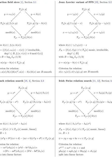
The function field sieve, due to Adleman [1], and its successors are the best algorithms for computing discrete logarithms in finite fields of small characteristic. The function field sieve gets its name from the fact that relations are produced with the help of two different function fields, a strategy originally developed in the number field sieve (which is good for factoring integers and computing discrete logarithms in finite fields of large characteristic) and subsequently adapted to finite fields of small characteristic. By searching for half-relations in each of the function fields and then combining them into full relations afterwards, one is able to reduce the degree of the polynomials that are required to be smooth, thus increasing the smoothness probability. This leads to a relation collection phase of complexityL(1/3), as opposed toL(1/2) above. The individual logarithm phase is also modified so that it has complexity L(1/3). The individual logarithm is computed with a so-called descent strategy, where loggh is first written as a sum of logarithms of elements of moderate degree, and then one proceeds recursively, writing each summand as a sum of logarithms of elements of smaller degree, until one finally arrives at a sum of logarithms of elements of small enough degree (i.e. all lying in the factor base). Combining these two speed-ups, one gets an algorithm of overall complexity L(1/3). We now give some more details of the relation collection phase, which can best be explained with the help of the commutative diagram given in Figure1, whereK=Fq and the fieldL=Fqn on the bottom is
the field where the discrete logarithm is to be computed.
In order to produce relations, one starts with a polynomial φ ∈Fq[x, y], typically of shape
φ(x, y) =a(x)y+b(x), and maps it viaψ1 and ψ2 into O1 andO2, respectively. Ifψ1(φ)∈ O1
andψ2(φ)∈ O2 are both B-smooth, then one maps both of these elements into Fqn viaη1 and
η2, where they produce a relation of the form
Figure 1: Commutative diagram illustrating relation collection phase of FFS and its successors
K[x, y]
O1=K[x, y]/f1(x, y) O2=K[x, y]/f2(x, y)
L=K[x]/k(x)
ψ1 ψ2
η2 η1
due to the commutativity of the diagram. The function fields involved are Fi = Quot(Oi) ⊇
Oi, i= 1,2.
3.1
The original function field sieve
Applicability. The function field sieve computes discrete logarithms in a fieldFqn=Fq[x]/k(x)
(withk monic and irreducible of degree n) of small characteristic, meaning thatq≤Lqn(1/3).
WriteK=Fq andL=Fqn.
Function fields. The function field sieve usually choosesf1monic inyof degreed(a parameter
to be optimized in the complexity analysis) and of degree O(1) inx, andf2(x, y) = y−h(x)
where hhas degree n/d. It is further required thatf1(x, h(x))≡0 modk, since this allows to
define the maps in the way specified below.
Thus the function fields involved are F1 = Quot(O1) = Fq(x)[y]/f1(x, y), an extension of
Fq(x) of degreed, andF2= Quot(O2) =Fq(x)[y]/f2(x, y), which is in fact the rational function
field Fq(x), since it is a degree 1 extension of Fq(x). Let us write Oi = Fq[x, αi(x)] with
fi(x, αi(x)) = 0 fori= 1,2, and notice thatα2=h.
Maps. We haveψ1 :y 7→α1(x), ψ2 :y7→h(x) and ηi :P(x, αi(x))7→P(x, h(x)). Notice that
theηi are well-defined since we havefi(x, h(x))≡0 modk.
Factor base. Since theOiare in general not unique factorization domains, one considers ideals,
which factor uniquely. Hence one defines the factor base in terms of ideals inOi:
FB(i)={h`(x), αi(x)−r(x)i |`irreducible, deg`≤B, fi(x, r(x))≡0 mod`(x)}
andFB=F
(1)
B ∪ F
(2)
B .
Relations. In order to produce relations, one picksφ=a(x)y−b(x)∈Fq[x, y] with dega,degb≤
efor some sieving parametere(to be optimized in the complexity analysis). One imposes further thataandbare coprime in order to avoid pairs (a, b) which are multiples of each other. We have
ψi(φ) =a(x)αi(x)−b(x), and it is easy to see that the ideal (a(x)αi(x)−b(x))Oiis smooth with
respect to the factor baseFB(i)if and only if the norm NFi|Fq(x)(a(x)αi(x)−b(x)) isB-smooth
as a polynomial (note that this is a polynomial, sinceaαi−bis a polynomial). Furthermore, we
have
NFi|Fq(x)(a(x)αi(x)−b(x)) = Resy(a(x)y−b(x), fi) =f
(h)
wherefi(h)(a, b) =fi(a/b)bdegfi is the homogenization offi, regarded as a polynomial iny.
By sieving, we find enough pairs (a, b)∈ Fq[x]2 such thatf
(h)
i (a, b) areB-smooth for both
i= 1,2; such pairs are calleddoubly B-smooth. By raising the decompositions to the respective class numbers, we obtain factorizations into principal ideals, or equivalently by looking at the generators of the ideals, half-relations in Oi, which can then be mapped via ηi into Fqn, thus
producing full relations there. For the many technical details we are skipping here, see e.g. [3].
Descent. In a first step, the descent rewrites the sought after logarithm as a sum of logarithms ofL(2/3)-smooth elements. Then it recursively descends the elements in the sum to elements of
FB by sieving elements of a lattice.
Complexity. Choose e = B = logqLqn(1/3) such that |FB| = Lqn(1/3), and choose d =
nlogq
logn
1/3
. Working out the constants as shown e.g. in [3, Chapter 7.5], the function field sieve
has a total complexity ofLqn(1/3,(32/9)1/3).
3.2
The Joux–Lercier variant of the function field sieve
Joux and Lercier [19] give a simplified version of FFS, where the function fields are no longer visible as such, though they are still present “in the background” as described above, and one no longer has to deal with ideals.
Applicability. As before, this variant of the function field sieve applies to fields Fqn =
Fq[x]/k(x), and we writeK=Fq, L=Fqn.
Function fields. Let f1(x, y) = γ1(y)−x and f2(x, y) = y−γ2(x) for γi of degree di with
d1d2≥n, and assume thatk|γ1(γ2(x))−x.
The function fields involved areF1=Fq(x)[y]/(γ1(y)−x), an extension ofFq(x) of degreed1,
andF2=Fq(x)[y]/(y−γ2(x)), which is in fact the rational function field (since it is a degree 1
extension ofFq(x)). Hence as above, there is one rational side.
Interpreting F1 as Fq(y)[x]/(γ1(y)−x), which is the rational function field iny, one might
even say that this algorithm has two rational sides.
Maps. We have ψ1 :y 7→γ2(x), ψ2 : x7→γ1(y) andη1: x7→γ1(γ2(x)) =γ1(η2(y)), η2: y 7→
γ2(x).
Factor base. Define
FB ={`(x), `(y)|`∈Fq[x] monic, irreducible, deg`≤B}.
Relations. By sieving (as above), findφ(x, y) =a(x)y−b(x)∈Fq[x, y] such thatφ(x, γ2(x)) and φ(γ1(y), y) are bothB-smooth. Suchφgive relations sinceφ(x, γ2(x)) =φ(x, y) =φ(γ1(y), y).
Descent. This is the same as for the function field sieve.
Complexity. This is also the same as for the function field sieve.
3.3
The L(1/4) algorithm
L(1/4 +o(1)), which was subsequently improved toL(1/4) in [10]. Finally, Granger, Kleinjung, and Zumbr¨agel took some steps in the direction of a provable complexity result by suggesting an alternative descent method in [12]. Most of these papers also present record breaking computa-tions. The differences between these algorithms lie mostly in the individual logarithm (descent) phase, while they share very similar strategies for relation collection. Therefore, we present the basic ideas of all of them together in this section. We point out though that [9,10,11,12] limit themselves to fields of characteristic two.
Applicability. The algorithms apply to fields Fqmn, where q ≈ n and m is small and fixed
([18, 4] consider onlym = 2). Hence a given field must be embedded into a finite field of this shape as a first step. WritingK=Fqm andL=Fqmn, the relation collection phase can also be
described via the diagram in Figure1.
Function fields. Let f1(x, y) =y−xq andf2(x, y) = h1(x)y−h0(x) (respectivelyf2(x, y) = h1(y)x−h0(y)) for polynomials h0, h1 ∈Fq[x] of small, constant degree. Experiments suggest
that suitableh0, h1of degree at most 2 always exist, see [18].
Writing Fqmn =Fqm[x]/k(x), [18, 4] require thatk |h1(x)xq−h0(x), while [11, 12] require
thatk|h1(xq)x−h0(xq), where the latter allows a slightly larger class of fields to be embedded
intoFqmn than the former.
We haveO1∼=Fqm[x] andO2∼=Fqm[x,1/h1(x)] (respectivelyO2∼=Fqm[y,1/h1(y)]), and the
function fields areFi= Quot(Oi), which are both degree one extensions ofFqm(x) (respectively
F2is a degree one extension ofFqm(y)), i.e. they are the rational function field themselves.
Maps. Let ψ1 : y 7→xq andψ2 :y 7→h0(x)/h1(x) (respectivelyx7→h0(y)/h1(y)), and let η1
andη2 be reduction modulok.
Factor base. SetB = 1, the factor base consists of all monic linear polynomials overFqm. Notice
that [18] includes also quadratic polynomials for technical reasons concerning the descent, we disregard this here.
Relations. The approach of [18, 4] can be interpreted as follows. Start with a polynomial of the shape φ = (aqy +bq)(cx+d)−(ax+b)(cqy +dq) for (a, b, c, d) ∈
F4qm \Fq4. Then
on the left (meaning ψ1(φ) ∈ O1), this splits completely: set y 7→ xq and use the identity F(x)qG(x)−F(x)G(x)q =G(x)Q
α∈Fq(F(x)−αG(x)) forF, G∈Fqm[x]. On the right (meaning
ψ2(φ)∈ O2), this becomes a polynomial of small, constant degree and therefore has high splitting
probability (for this purpose,h1 is included in FB by definition). We get a relation as soon as
the right-hand-side is smooth.
The other papers start with a polynomial φ =xy+ay+bx+c ∈Fqm[x, y] and map it to
both sides. On the left, the resulting polynomial is of the form ψ1(φ) = xq+1+axq+bx+c,
and it can be shown (using a transformation resulting in a polynomial of shapexq+1+Dx+D
and results of Bluher [2] and Helleseth–Kholosha [15] on the splitting probability of polynomials of this shape, see [9]) that such polynomials split with probability q−3, which is much higher than the splitting probability given by Theorem1 for random polynomials of the same degree. A parametrization of such polynomials which split completely is also given. On the right, again, the polynomialψ2(φ) splits with large constant probability.
Descent. We skip this, since it is different in all the papers mentioned above.
Complexity. Sincen≈qandmis small and fixed, we have thatqmis polynomial in the input
sizeqmn. Then the relation generation takes only polynomial time, since the splitting probability
3.4
Comparison
A schematic comparison of the relation collection phase for all algorithms discussed in this section is given in Figure2.
4
Algebraic curves
The algorithm of Enge, Gaudry, and Thom´e [7,8] is the most efficient currently known algorithm to compute discrete logarithms in Jacobians of algebraic curves. It has complexityL(1/3), but it is important that this improvement over theL(1/2) algorithm presented in Section2is not due to the search of relations in two different function fields, but rather to the bounds on the degrees of the curve equation, which are due to the fact that the algorithm applies only toCab-curves.
Applicability. The algorithm applies to so-calledCab-curves defined overFq by an equation
Cab:ya+xb+f(x, y) = 0,
such that the affine part of the curve is smooth, and where gcd(a, b) = 1 and ai+bj≤ab for all monomials xiyj of f. Such curves have genusg = (a−1)(b−1)/2. The DLP is defined in
its Jacobian JacCab(Fq), which has size aboutq
g. The elements of the Jacobian are degree zero
divisor classes, which we denote by [D] for a divisorD.
Function field. There is only one function field involved in the relation search, namely the function field Fq(Cab) =Fq(x)[y]/(ya+xb+f(x, y)) of the curve. It is a degree aextension of
Fq(x).
Factor base. The factor base consists of all prime divisors on the curve of degree at mostB, whereB= logqLqg(1/3) is chosen such that the factor base has sizeLqg(1/3).
Relations. One searches for polynomial functions φ ∈Fq(Cab) such that div(φ) is B-smooth.
If div(φ) =Pν
iPi withPi ∈ FB, then Pνi[Pi] = 0 gives a relation in JacCab. Smoothness of a
divisor can be tested by checking if NFq(Cab)|Fq(x)(φ)∈Fq(x), and actually ∈Fq[x] since φ is a
polynomial function, isB-smooth. Notice that NFq(Cab)|Fq(x)(φ) = Resy(φ(x, y), y
a+xb+f(x, y))
and can therefore easily be computed as a resultant.
Descent. The algorithm recursively descends a place of degreeg1/3+τ, τ ∈[0,2/3], to a sum
of places of degree g1/3+τ /2 by sieving elements of a lattice. Notice that there is no initial
smoothing.
Complexity. Choosing a ≈ gα, b ≈ g1−α for α ∈ [1/3,2/3], and degyφ ≈ gα−1/3,degxφ ≈
g2/3−α, one can estimate
degx NFq(Cab)|Fq(x)(φ)
≤g2/3,
hence the norm (and therefore div(φ)) is B-smooth with probability Lqg(1/3)−1. Hence one
can collect |FB|=Lqg(1/3) relations in time Lqg(1/3), and the linear system can be solved in
the same time. The descent phase has the same complexity, and therefore we get an overall complexity ofLqg(1/3), whereq andggrow to infinity.
5
Ideas for a faster relation generation phase for curves
Figure 2: Comparison relation search of FFS and its successors
Function field sieve[1], Section3.1
Fq[x, y]
Fq[x, y]/f1(x, y) Fq[x, y]/(y−h(x))
Fqn=Fq[x]/k(x)
y7→α1(x) y7→h(x)
modk(x) modk(x)
wherek(x)|f1(x, h(x))
FB={h`(x), αi(x)−r(x)i |`irreducible,
deg`≤B, fi(x, r(x))≡0 mod`(x)}
withB= logqLqn(1/3)
φ=a(x)y−b(x)∈Fq[x, y]
Criterion for relation:
f1(x, a(x)/b(x))b(x)d, a(x)−b(x)h(x) areB-smooth
Joux–Lercier variant of FFS[19], Section3.2
Fq[x, y]
Fq[x, y]/(γ1(y)−x) Fq[x, y]/(y−γ2(x))
Fqn=Fq[x]/k(x)
y7→γ2(x) x7→γ1(y)
y7→γ2(x)
x7→γ1(γ2(x))
where k(x)|γ1(γ2(x))−x
FB ={`(x), `(y)|`∈Fq[x] monic, irreducible,
deg`≤B}
with B= logqLqn(1/3)
φ=a(x)y−b(x)∈Fq[x, y]
Criterion for relation:
φ(x, γ2(x)), φ(γ1(y), y) areB-smooth
French relation search[18, 4], Section3.3
Fq2[x, y]
Fq2[x, y]/(y−xq) Fq2[x, y]/(h1(x)y−h0(x))
Fq2n=Fq2[x]/k(x)
y7→xq y7→h0(x)/h1(x)
modk(x) modk(x)
wherek(x)|h1(x)xq−h0(x)
FB={`(x)|`∈Fq2[x] monic, linear}
i.e.B= 1
φ= (aqy+bq)(cx+d)−(ax+b)(cqy+dq)∈Fq2[x, y]
Criterion for relation: (aqc−acq)xh
0(x) + (aqd−bcq)h0(x)+
+(bqc−adq)xh1(x) + (bqd−bdq)h1(x)
Irish–Swiss relation search[11,12], Section3.3
Fqm[x, y]
Fqm[x, y]/(y−xq) Fqm[x, y]/(h1(y)x−h0(y))
Fqmn=Fqm[x]/k(x)
y7→xq x7→h0(y)/h1(y)
modk(x) modk(x)
where k(x)|h1(xq)x−h0(xq)
FB ={`(x), `(y)|`∈Fqm[x] monic, linear}
i.e. B= 1
φ=xy+ay+bx+c∈Fqm[x, y]
Criterion for relation:
xq+1+axq+bx+cand
point of view and try to amplify relations (e.g. via homographies), or that of the Irish–Swiss team of finding families of functions that have higher-than-usual splitting probability. In both cases, the shape of the function field plays a crucial role, and the new algorithms profit precisely from this freedom to choose convenient function fields.
In the case of algebraic curves, the function field is given by the curve in question, and there is unfortunately no freedom to choose it. Therefore, we ask ourselves instead whether there exist curves (with corresponding function fields) for which we are easily able to produce relations. The curves should, of course, have no known weaknesses with respect to the DLP. In particular, they should not be supersingular, or more generally, not have a Jacobian of smooth order, they should not have small embedding degree, and they should obviously not have genus 0. In fact, in order to mimic the finite field algorithms, we would need a curve defined overFq of genus aboutq, so
that the Jacobian has order aboutqq.
A more precise formulation of the question we wish to answer is the following. We write poly(q) =qΘ(1).
Question 1. Let C be a projective curve defined over Fq of degree poly(q). Under which
con-ditions is the number of polynomial functions of degree O(1) defining divisors which split into factors of degreeO(1) unexpectedly large, say of the formpoly(q)?
Unfortunately our impression is that there may not exist curves which satisfy all of these criteria. A precise formulation of this impression is given in Section 7, but before we get to it, we explain the reasoning and experiments that led to this conclusion.
A first observation is that the function fields chosen in theL(1/4) algorithms for finite fields are not interesting in our context, since the corresponding curvesy−xq andh1(x)y+h0(x) both have genus zero.
We tried two approaches, corresponding to the point of view of Joux (and the “French team”) and that of the “Irish–Swiss team”, respectively.
The first approach would be to find a curve, together with one smooth function, which gives a relation, and to then amplify this into many relations using homographies. This works well for the specific curve y−xq, since it is of particularly simple shape, as shown in Example 1.
For curves with more complicated equations, this becomes more difficult, as the application of the homography is no longer compatible with taking the resultant. Example 2 shows a curve where this approach does not work, i.e. where we find exactly two polynomial functions that have smooth principal divisors but no more.
The second approach would be to find a curve, together with a (parametrized) family of smooth functions, such that the (parametrized) resultant has high splitting probability. Again, this works well for the curve y−xq, since we have Resy(φ(x, y), y−xq) = νφ(x, xq) for some
constant ν, and therefore the norm of φ depends on φ in a very simple way. For this reason, simple φ’s produce simple N(φ)’s, and it is easy to produce polynomials for which results on higher splitting probability are known, see Example 1. The difficulty about generalizing this approach is that there exist few known families of polynomials with high splitting probability, and it is difficult to produce these few very simple polynomials with more interesting curves.
Example 1. LetC:y−xq = 0 andφ(x, y) =y−x∈
Fq(C). Then
NFq(C)|Fq(x)(φ) = Resy(y−x, y−x
q) =ν(xq−x) =ν Y
α∈Fq
(x−α)
In order to amplify this one relation into many, Joux proposes to apply a homography x7→
ax+b
cx+d, where a, b, c, d∈Fq2. After multiplication by (cx+d)q+1, this gives
(ax+b)q(cx+d)−(ax+b)(cx+d)q = (cx+d) Y
α∈Fq
((a−αc)x+ (b−αd)),
and one has found many polynomials that split into linear factors. How many? As many as
there are matrices
a b c d
∈PGL2(Fq2)/PGL2(Fq), which has cardinality q3+q.
Interpreting this in terms of relations on the curveC, we “apply” the homography toφ(x, y) =
y−xas follows. Setting
φhom(x, y) = (aqy+bq)(cx+d)−(ax+b)(cqy+dq),
we get
Resy(φhom(x, y), y−xq) =ν(cx+d)
Y
α∈Fq
((a−αc)x+ (b−αd))
for a constantν, which gives aboutq3 different relations in Jac
C.
Alternatively, we may defineφ(x, y) =xy+ay+bx+cfora, b, c, d∈Fqm, which gives
Resy(φ(x, y), y−xq) =xq+1+axq+bx+c.
Ifc6=abandb=6 aq, then the transformationx7→ ab+c
b+aqx+amaps the result tox
q+1−Dx+D
which, for D ∈ Fqm, splits into linear factors for about qm−3 values of D according to [2,
Lemma 4.4]. In other words,φhas splitting probabilityq−3, which is much higher than that of
a random polynomial of degreeq+ 1, which is on the order ofq−q according to Theorem1.
The connection between the two approaches, and an interesting observation, is that poly-nomials (ax+b)q(cx+d)−(ax+b)(cx+d)q are of the form Axq+1+Bxq +Cx+D, and
such polynomials have splitting probabilityq−3 according to [2], which is higher than expected.
It is possible that this phenomenon holds more generally. For example, (ax2+bx+c)q(dx2+
ex+f)−(ax2+bx+c)(dx2+ex+f)q splits completely into factors of degree 2 and has terms
x2q+2, x2q+1, x2q, xq+2, xq+1, xq, x2, x,1, so one might expect that polynomialsAx2q+2+Bx2q+1+
Cx2q+Dxq+2+Exq+1+F xq+Gx2+Hx+Isplit into quadratic factors with higher probability than expected. Counting arguments as well as experiments for m= 2 and small fields suggest that this may be the case with probabilityq−7, but such counting experiments are only possible
for very small fields and therefore only give a vague idea, and we are not aware of any results similar to those of [2, 15] for such polynomials. If such a thing were true, we could search for pairs of C, φsuch that the resultant has such a shape. Notice that it is obviously possible to extend this idea, using e.g. polynomials of larger degrees and possibly products of polynomials of different degrees.
6
Experiments
Example 2. Consider C : y2−xq+1+ 2x−1 = 0, which is a hyperelliptic, non-supersingular
curve of genusg= (q−1)/2, andφ(x, y) =y−x+ 1. Then
Resy(φ, y2−xq+1+ 2x−1) =x(xq−x)
and therefore splits into linear factors. However, exhaustive search shows that the only functions of the form ψ =axy+by+cx+dwith a, b, c, d ∈ Fq2 such that Resy(ψ, y2−xq+1+ 2x−1) splits into linear factors and produces a non-trivial relation are ψ = y+x−1, y−x+ 1, for
q= 7,11,19,23 (notice that these are all primes ≡3 mod 4). For these values ofψ, we have
Resy(ψ, y2−xq+1+ 2x−1) =x(xq−x).
Therefore, for this curve and the values of q mentioned above, there is no way of applying a homography appropriately toφor of findingψ with higher splitting probability.
Example 3. LetC:y2−xq−1+ 1 = 0, which is a hyperelliptic, non-supersingular curve of genus
g= (q−3)/2. In fact, it is a CM-curve and has 2q−2 automorphisms. We look for a polynomial functionφ∈Fq(C) such that Resy(φ, y2−xq−1+ 1) =xq−xor a small multiple thereof. Since
the curve equation is quadratic in y, the function must be of shape φ(x, y) = φ1(x)y+φ0(x). Furthermore, the degrees of φ0 and φ1 should be very small. If we allow degree at most one,
then by solving
Resy(φ1(x)y+φ0(x), y2−xq−1+ 1) = (xq−x)(x+a)
for somea, we geta= 0, φ0=x, φ1= 0 and thereforeφ(x, y) =xy. This is not interesting, asφ
is not irreducible.
If we allow φ0, φ1 of degree up to two, then with the same reasoning, we get φ(x, y) = (x2+ax)yfor any choice ofa. Again, this is not interesting as it is not irreducible.
Example 4. Let C : y2−xq−2+x+ 1 = 0, which is a hyperelliptic, non-supersingular curve of genus g = (q−3)/2. As in Example 3, we try to find a function φ =φ1(x)y+φ0(x) such that Res(φ, y2−xq−2+x+ 1) is a multiple ofxq−xby some linear factors. Trying to solve the equation, we find that neither linear nor quadraticφ0, φ1 produce a resultant which is divisible byxq−x. The same is true forC:y2−xq−1−1 and many other curves.
Example 5. LetC : y2+y =xn be a Koblitz–Buhler curve (see [5]), which is a hyperelliptic
curve. Its equation can be transformed intoy2=xn+ 3/4 via the transformation y 7→y−1/2
in odd characteristic. For this curve, which functions split overFq[x] depends on q. For some
values ofq(e.g. q= 7), we can show that there are noφ0, φ1of degree 2 such that Resy(φ1(x)y+
φ0(x), y2+y =xn) =xq−xby solving the corresponding polynomial system with coefficients
of theφi as indeterminates.
Example 6. Consider the Hermitian curveC :xq+1+yq+1−1 = 0. These curves have genus g=q(q−1)/2 and are known for the fact that they have manyFq2-rational points, more precisely, exactlyq3+ 1. In other words, the function fieldFq2(C) is maximal (in the sense that the upper Hasse–Weil bound on the number of places of degree one is attained). For this reason, such curves are of interest e.g. in coding theory. It is also known that Hermitian curves are supersingular, and therefore not interesting in the context of cryptography. For more on Hermitian curves, see e.g. [21, Chapter VI, VII].
Now let φ = xy+ay+bx2+cx+d with a, b, c, d ∈
for a random function of the same degree (here, the splitting probability behaves like q−q for
q→ ∞). However, experiments also show that special things are happening here: If the resultant is 2-smooth, then it is always automatically already 1-smooth (i.e. we did not find functions that produced a resultant which was 2-smooth but not 1-smooth).
Example 7. Let C : yq+1 +xq+1y −1 = 0, which is a non-hyperelliptic, non-supersingular curve of genus g=q(q+ 1)/2. Experiments for q = 5,7,11,13,17,19,23 show that there is no irreducible functionφ=xy+ay+bx+c∈Fq2[x, y] such that Resy(φ, yq+1+xq+1y−1) splits
completely into linear factors.
7
A possible obstruction
A possible conclusion from the experiments described in Section 6 is that curves for which principal divisors with higher-than-expected splitting probability exist are very special, and in fact, so special that the DLP is already known to be easy for these curves. A more precise formulation and possible answer to Question1is the following.
Conjecture 1. Let(Cq)q be a family of projective curves defined overFq of genuspoly(q), given
by an equation of degree poly(q). Assume that there existpoly(q)monic, irreducible polynomial functionsφ∈Fq2(Cq)of degree O(1) such that div(φ)is O(1)-smooth. Then JacCq is isogenous
to a product of elliptic curves, for large enoughq.
The main example supporting this conjecture are Hermitian curves, which are supersingular and therefore, in particular, have a Jacobian isogenous to a product of supersingular elliptic curves.
It is a priori not clear how to prove such a statement, since one would have to relate splitting probabilities of rational functions to the structure of the Jacobian of a curve. However, there are some results related to the special case of Question1where we set both constants equal to one:
Question 2. Let C be a projective curve defined over Fq of degree poly(q). Under which
con-ditions is the number of lines defining divisors which split completely unexpectedly large, say of the formpoly(q)?
Heuristically, for a curve of degreed, we expect aboutq2/d! such divisors to split completely.
Moreover, for reflexive curves of fixed degreed≥3, it has been proven by Diem that this count holds asymptotically:
Theorem 3([6, Theorem 3]). Letd≥3 be fixed, and letC be a projective curve of genus at least one given by a plane model of degreed. If d >4, then assume that the plane model is reflexive. Then the number of divisors onC that are given by lines inP2 and split completely into distinct
points is in d1!q2+O(q3/2).
For example, Hermitian curves are non-reflexive, and as explained in Example 6, they have many points. This corresponds to the fact that there are many divisors given by lines, and therefore also many that split.
Since we are interested in curves where there are rational functions with higher-than-expected splitting probability, this rules out reflexive curves as possible candidates. This leaves non-reflexive curves, which are relatively well-studied in the literature, see e.g. [13,14].
most varieties are reflexive. The main examples for non-reflexive varieties are strange curves, which have the property that all tangents pass through a common point.
In fact, non-reflexive curves are so special that they have been classified according to their degree by Ballico and Hefez [14]. Among other things, they show that for non-reflexive plane curvesCof degreedwith “moderate singularities” defined over fields of characteristicp >2, we always havep|d−1. Moreover, for such curves, they give the following result.
Theorem 4([14, Proposition 1]). Any non-reflexive plane curve of degreed=q+ 1≥4, forqa power of the characteristic of the field of definition, and of genus greater than zero is projectively equivalent to the curve
xq+1+yq+1+zq+1= 0. (1)
These are the Hermitian curves, which are known to be supersingular. As discussed earlier, such curves are not interesting in our context. Summarizing, because of Diem’s theorem, the only curves which are candidates in response to Question 2 are non-reflexive curves, but such curves are not interesting in our context. This is in accordance with our experiments, in which we found only curves of shape (1).
The question that remains is whether a more general statement, perhaps along the lines of our conjecture, can be proven in response to the more general Question1. One possible approach to this would be to use Cebotarev’s density theorem, which is the main argument in the proof of Diem’s theorem.
8
Conclusion
Our investigation of possible ways of adapting the relation collection phase of the new L(1/4) and quasi-polynomial algorithms to algebraic curves suggests that this is a difficult problem. In particular, our experiments indicate that curves which permit rational functions whose principal divisors have higher-than-expected splitting probability are very special and therefore not inter-esting in our context, since the DLP in these curves is already known to be weak. We conjecture that this is always true and show that a special case of this conjecture can be proven using known results of Diem and Ballico–Hefez. If the more general statement could be proven, this would rule out a more general approach that allows polynomial functions of constant degree and the corresponding divisors to split into factors of constant degree. Clearly, this would still not mean that there is noL(1/4) DLP algorithm for Jacobians of curves, it would mean simply that one needs to investigate more sophisticated ideas than the rather obvious analogy we have considered here.
References
[1] L. M. Adleman. The function field sieve. InAlgorithmic Number Theory (ANTS I), volume 877 ofLNCS, pages 108–121. Springer, 1994.
[2] A. W. Bluher. Onxq+1+ax+b. Finite Fields Appl., 10:285–305, 2004.
[3] R. B˘arbulescu.Algorithmes de logarithmes discrets dans les corps finis. PhD thesis, Univer-sit´e de Lorraine, Available athttp://tel.archives-ouvertes.fr/tel-00925228/file/ these_avec_resume.pdf, 2013.
editors,Advances in Cryptology: Proceedings of EUROCRYPT ’14, volume 8441 ofLNCS, pages 1–16. Springer, 2014.
[5] J. Buhler and N. Koblitz. Lattice basis reduction, Jacobi sums and hyperelliptic cryptosys-tems. Bull. Aust. Math. Soc., 58:147–154, 1998.
[6] C. Diem. On the discrete logarithm problem for plane curves. J. Th´eor. Nombres Bordeaux, 24:639–667, 2012.
[7] A. Enge and P. Gaudry. AnL(1/3 +ε) algorithm for the discrete logarithm problem for low degree curves. In M. Naor, editor,Advances in Cryptology: Proceedings of EUROCRYPT ’07, volume 4515 ofLNCS, pages 379–393. Springer, 2007.
[8] A. Enge, P. Gaudry, and E. Thom´e. AnL(1/3) discrete logarithm algorithm for low degree curves. J. Cryptology, 24:24–41, 2011.
[9] F. G¨olo˘glu, R. Granger, G. McGuire, and J. Zumbr¨agel. On the function field sieve and the impact of higher splitting probabilities. In R. Canetti and J. A. Garay, editors,Advances in Cryptology: Proceedings of CRYPTO ’13, volume 8043 ofLNCS, pages 109–128. Springer, 2013.
[10] F. G¨olo˘glu, R. Granger, G. McGuire, and J. Zumbr¨agel. Solving a 6120-bit DLP on a desktop computer. In T. Lange, K. Lauter, and P. Lisonˇek, editors,Proceedings of SAC ’13, LNCS, pages 136–152. Springer, 2013.
[11] R. Granger, T. Kleinjung, and J. Zumbr¨agel. Breaking ‘128-bit secure’ supersingular binary curves. In J. A. Garay and R. Gennaro, editors, Advances in Cryptology: Proceedings of CRYPTO ’14, volume 8617 ofLNCS, pages 126–145. Springer, 2014.
[12] R. Granger, T. Kleinjung, and J. Zumbr¨agel. On the powers of 2. Available at http: //eprint.iacr.org/2014/300, 2014.
[13] A. Hefez. Non-reflexive curves. Compos. Math., 69:3–35, 1988.
[14] A. Hefez and E. Ballico. Non-reflexive projective curves of low degree. Manuscripta Math., 70:385–396, 1991.
[15] T. Helleseth and A. Kholosha. x2l
+x+a and related affine polynomials over GF(2k).
Cryptogr. Commun., 2(1):85–109, 2010.
[16] F. Heß. Computing relations in divisor class groups of algebraic curves over finite fields. Available athttp://www.staff.uni-oldenburg.de/florian.hess/publications/dlog. pdf, 2002.
[17] F. Heß. Computing Riemann–Roch spaces in algebraic function fields and related topics. J. Symbolic Comput., 33:425–445, 2002.
[18] A. Joux. A new index calculus algorithm with complexityL(1/4 +o(1)) in small character-istic. In T. Lange, K. Lauter, and P. Lisonˇek, editors,Proceedings of SAC ’13, LNCS, pages 355–379. Springer, 2013.
[20] A. M. Odlyzko. Discrete logarithms in finite fields and their cryptographic significance. In T. Beth, N. Cot, and I. Ingemarsson, editors, Advances in Cryptology: Proceedings of EUROCRYPT ’84, volume 209 ofLNCS, pages 224–314. Springer, 1984.