ISSN 2286-4822 www.euacademic.org
Impact Factor: 3.4546 (UIF) DRJI Value: 5.9 (B+)
Performance Evaluation and Comparison of the
BPTC using a new Soft Hamming Decoder
ALAA A. GHAITH
HKS Laboratory - Electronics and Physics Dept. Faculty of Sciences I - Lebanese University Lebanon
HAMZÉ H. ALAEDDINE
HKS Laboratory - Electronics and Physics Dept. Faculty of Sciences I - Lebanese University Lebanon
Abstract:
a design of soft decoding of the BPTC system, which is composed of two, similar or different, Hamming block code combinations, a block interleaving, and a BPSK modulation, over an AWGN channel. Different schemes were simulated to observe its coding improvement, and compare the bit error rate (BER) for different soft decoding of the BPTC.
Key words: Syndrome based soft decoding, Hamming Code, soft-output, BPTC, AWGN, block interleaver, coding gain, turbo code.
1. INTRODUCTION
Concatenated coding schemes were first proposed by Forney [Forney 1966] as a method for achieving large coding gains by combining two or more relatively simple block or component codes. The resulting codes had the error-correction capability of much longer codes, and they were endowed with a structure that permitted relatively easy to moderately complex decoding. A serial concatenation of codes is most often used for power-limited systems. The most popular of these schemes consists of a Reed-Solomon outer (applied first, removed last) code followed by a convolutional inner (applied last, removed first) code. A turbo code [Berrou 1993] can be thought of as a refinement of the concatenated encoding structure plus an iterative algorithm for decoding the associated code sequence. Turbo codes were first introduced in 1993 by Berrou, and Glavieux, where a scheme is described that achieves a bit-error probability of 10-5
using a rate 1/2 code over an AWGN channel and BPSK modulation at an Eb/N0 of 0.7 dB. The codes are constructed by
the BPTC using a new Soft Hamming Decoder
best exploit the information learned from each decoder, the decoding algorithm must effect an exchange of soft decisions rather than hard decisions. For a system with two component codes, the concept behind turbo decoding is to pass soft decisions from the output of one decoder to the input of the other decoder, and to iterate this process several times so as to produce more reliable decisions. The purpose was to find digital communications systems that have a capacity and a performance close to the limits found by Shannon. For applications that require error correcting codes to operate with much shorter delays, Berrou, Evano, and Battail have advocated block component codes, maintaining turbo coding decoding principle. These codes, called turbo- block codes, exhibit a coding gain that is considerably larger than that of the standalone component block codes [Divsalar 2001]. Moreover, the decoding complexity for these turbo-block codes is quite reasonable, as long as the decoding complexity of the component block codes is so [Divsalar 2004]. The block product turbo code (BPTC) is classified as one of block turbo code concatenation forms. The Hamming code can detect two-bit error or correct one-bit error [Li 2004]. The BPTC uses two Hamming codes for "column" coding and "row" coding, it has improved the Hamming code correcting only one error. In addition, the BPTC carries out block interleaving coding for disorganizing the transmission sequence before transmission, so as to avoid burst errors [Li 2004] and [Huang 2007].
turbo principal process which will provide a lot of gain when compared to the turbo hard decision decoder and to the single soft decoder [Chen 2011] and [Megha 2014].
The remainder of this paper is organized as follows. In Section 2, we discuss the background about the Hamming codes. Section 3 presents the syndrome based soft, and the soft decoding technique. The system design of the BPTC coding and decoding schemes are also presented in Section 4. The system performance is investigated in Section 5 through extensive trace-driven simulation. Finally, conclusions are given in Section 6 along with the suggestions for future work.
2. THEORETICAL BACKGROUND
2.1. Encoding and Transmission
The encoding of the message bits' m can be performed by a modulo 2 vector matrix multiplication of m and the generator matrix G
c ≡ m.G (1)
The expression "≡" is equivalent with c = (m.G) modulo 2. Hamming code is an important forward error correction (FEC) in theory and practice so far. It is a sort of binary linear block code. It puts forward an important single-error-correcting code, using parity check matrix (H) to detect and correct errors. It is a simple type of systematic code, described as the following structure.
Block length: n = 2p–1
Number of data bits: k = 2p – p – 1 Number of check bits: n – k = p
Minimum distance: dmin = 3 Correct single bit error (n, k) = (2p – 1, 2p – 1 – p)
the BPTC using a new Soft Hamming Decoder kn k k n n
k V V V
V V V V V V V V V G 2 1 2 22 21 1 12 11 2 1
Among which, V1~Vk are linearly independent vectors that can generate all code vectors. The data of the transmitting terminal are usually expressed in column vectors, therefore, the sequence of k message bits, i.e. the message m is expressed as
1×k matrix.
The generator matrix of systematic (7, 4)-Hamming code is given by
P I G 1 0 1 1 1 1 1 1 0 0 1 1 | | | | 1 0 0 0 0 1 0 0 0 0 1 0 0 0 0 1
After the encoding, c is modulated, so that a logical zero is equivalent to a +1 and a logical one is equivalent to a -1,
1
x . The modulated signal x is distorted by the additive
white Gaussian noise (AWGN) w and results in the receive signal y,
y = x + w (2)
2.2. Hard Decision Decoding
In order to decode the received signals, we need to define a parity check matrix and a syndrome. There is a (n-k) × n
matrix H in each generator matrix G, so that the columns of G
are orthogonal to the columns of H, i.e. G.HT=0, the HT is the
transpose matrix of H. In order to meet the orthogonality of system coding, the component of matrix H can be expressed as
T
k
n
P
I
H
|
. Therefore, the matrix HT can be expressed as T k n T P I H
c is the code word derived from matrix G if and only if c.HT = 0.
Let r be the vector received by the receiving terminal, so the r
it is the result of parity check implemented in r, judge whether
r is an element in the codeword set. Based on development of equation s = (c + e).HT = c.HT + e.HT. However, for all elements
in codeword set c.HT=0, therefore s = e.HT.
Since the correction capability of Hamming code is 1, meaning the error pattern is one selected from n. Error patterns with 2 (duets) or 3 errors (triplets) which belong to the same syndrome are not taken into account for the decoding and the distorted code word is corrected as follow:
1. Use s = r.HT to calculate the syndrome of r
2. Find out common first error pattern ej, its syndrome equals r.HT
3. This error pattern is supposed to be the error caused by channel
4. The identified receive correction vector or code word equals c = r + ej
In fact, every double error is decoded to a valid but wrong code word. This explains the poor performance of HDD for Hamming codes.
3. SOFT-OUTPUT DECODING
3.1. Syndrome Based Soft Decision Decoding
For the syndrome based soft decision decoding it is required to calculate the log-likelihood ratios (LLR) from the received signal y,
x y
P y x P y x L | 1 | 1 ln | (3)
which finally leads to
, 4 1 exp 1 exp ln | 0 2 0 2 0 y N E y N E y N E y x L b b b (4)
the BPTC using a new Soft Hamming Decoder
Let us assume that the syndrome of the distorted bit sequence of a (7,4)-Hamming code is s = (0 0 1). The possible error patterns are collected in matrix E with its elements ej,i
0 1 1 0 1 0 0 0 0 0 1 1 1 0 0 1 0 1 0 0 1 0 0 1 0 0 1 1 0 0 1 1 0 0 0 0 1 0 0 0 1 0 0 0 0 0 1 0 1 1 0 0 0 0 0 0 E
where the second to fourth row bears the duets and the fifth to eighth row bears the triplets. The error patterns for all syndromes are determined in advance and stored in a list. The size of the list rises quadratically for double errors and cubically for triple errors. Every row of E is multiplied by the absolute value of LLRs of the received signal L(x|y). Afterwards, the resulting row vector is added up. The vector with the lowest sum of LLR suggests the error pattern with the highest probability of a correct decoding.
3.2. Soft Decoding
The structure of the soft hamming decoder is shown in Fig. 1. In general, soft-output decoding provides output values for iterative or turbo decoding.
Figure 1: Soft-Output Hamming Decoder
In order to generate soft-outputs, the following algorithm is proposed. The probability values of a code word are given by
1 | ˆ 1 0 | ˆ ~ where ~ ~ , , j i j j j j i j j j j j j i e if y c c P e if y c c P P P P (6) Now is normalized, so that the sum of the normalizedprobabilities Pi over all rows i is equal to 1,
1
i iP
. So the probabilities Pi are given by
' ' ~ ~ i i i i P P P (7)Pi can be interpreted as the probability of correct decoding for the given error pattern of row i. In a last step, the probability that xj = +1, for a given received code word y, is calculated by
the sum of Pi over all rows i, if ei,j =
c
ˆ
j, wherec
ˆ
jis defined as the logical received bit sequence. The estimation of the new probabilities after the soft decoding.
j j i c e i ij y P
x P ˆ , | 1
ˆ (8)
Due to the normalization, so that
1
i i
P
, the probability of
x y
Pˆ j 1| can be calculated by
x y
P
x y
Pˆ j1| 1 ˆ j1| (9) In order to exchange the information for turbo decoding it is required to calculate L-values from the derived probabilities.
3.3. Some Simulation Results
the BPTC using a new Soft Hamming Decoder
Figure 2: (15,11)-Hamming code
Fig. 2 shows the bit error rate of the (15,11)-Hamming code for different types of decoding. It is shown that the decoding performance of the duet and triplet decoding is very close to the union bound which is an upper bound for the bit error probability after maximum likelihood decoding. For the evaluation we focus on a BER=10-4. The coding gain amounts to
0.9 dB for the HDD and 1.8 dB for the duet decoding. Further 0.25 dB can be gained by triplet decoding.
Nc Kc HDD Gain Duets Gain Triplets Gain
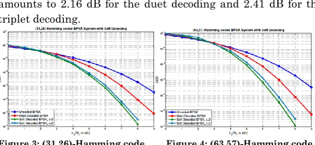
7 4 7.80 0.31 6.75 1.36 6.65 1.46 15 11 7.20 0.90 6.30 1.80 6.05 2.05 31 26 7.00 1.21 6.05 2.16 5.80 2.41 63 57 7.00 1.21 6.05 2.16 5.75 2.46 127 120 7.10 1.11 6.35 1.86 6.00 2.21
Table 1: Coding gain for Eb/N0 in dB for a BER=10-4.
The (31,26)-Hamming code obtained the results for codes, for duets as well as for triplets. Fig. 3 shows that the coding gain amounts to 2.16 dB for the duet decoding and 2.41 dB for the triplet decoding.
Quite a similar picture can be drawn for the (63,57)-Hamming code as shown in Fig. 4. The coding gain is similar to the (31,26)-Hamming code, but the bit error curve falls sharply. It is also shown that the difference between duet and triplet decoding is higher with 0.3 dB.
4. BPTC CODING AND DECODING SCHEMES
Hamming put forward an important error-correcting code, Hamming code in 1948. It uses parity check matrix (H) to detect and correct errors, however, its ability in detection and correction is limited, it can only detect 2-bit errors or correct 1-bit errors.
The block product turbo code (BPTC) is classified as one of block turbo code concatenation forms. The Hamming code can detect two-bit error or correct one-bit error. The BPTC uses two Hamming codes for "column" coding and "row" coding, it has improved the Hamming code correcting only one error. The encoder starts with the first row of information bits, calculates and appends the parity bits, and then moves on to the second row. This is repeated for each row. Next, the encoder starts with the first column of information bits, calculates and appends the parity bits for that column, and moves to the next column. Once the information block is complete, the encoder calculates and appends parity bits onto rows. It is important to note that different code lengths may be used for the horizontal and vertical blocks. In addition, the BPTC carries out block interleaving coding for disorganizing the transmission sequence before transmission, so as to avoid burst errors.
the BPTC using a new Soft Hamming Decoder
4.1. Encoder System Design
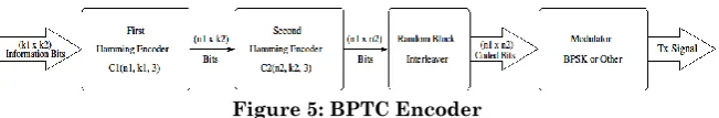
The general structure of a BPTC encoder is shown in Fig. 5. It consists of two systematic hamming encoders C1 and C2. It should be noted that the size of these two hamming codes could be the same and the free distance of any hamming code is always 3 which means it can correct one-bit error. The output sequences, however, are the same for identical input sequences. The N bit data block is first arranged in (k1 x k2) matrix form
before encoded by C1, an additional zero padding bits are placed at the end of the data block if needed. After encoded by the first encoder, the output block is then (n1 x k2) matrix after adding
the corresponding bits to each column. The output data block of the C1 is also encoded by C2 giving an output encoded data of (n1 x n2) matrix after adding the corresponding bits to each row.
Then this data block will be interleaved by a random interleaver. The main purpose of the interleaver is to randomize bursty error patterns so that it can be correctly decoded. It also helps to increase the minimum distance of the BPTC. The turbo coder obtained here can be described with the following structure.
Block length: N = n1 x n2
Number of data bits: K = k1 x k2
Number of check bits: P = (n1-k1) x k2 + (n2-k2) x k1 + k1 x k2
Coding Rate: R = K/N = R1 x R2.
4.2. Decoder System Design
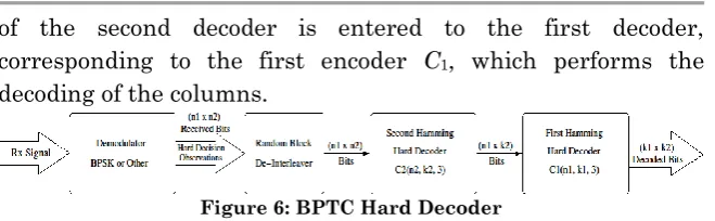
The decoding procedure described below is generalized by cascading elementary decoders illustrated in Fig. 6. Let us consider the decoding of the rows and columns of a product code described in Section 4.1 and transmitted on a Gaussian channel using BPSK signalling. On receiving (n1 x n2) matrix R
corresponding to a transmitted (k1 x k2) codeword E, the second
of the second decoder is entered to the first decoder, corresponding to the first encoder C1, which performs the decoding of the columns.
Figure 6: BPTC Hard Decoder
4.3. BPTC coding mechanism analysis
Although the BPTC is composed of Hamming code, its probability of being corrected in the second dimension coding is increased by using the fundamental characteristics of turbo code. So the correction capability will increase normally to more than three-bits error. But we should mention here that it is unfair to compare a simple hamming code with the corresponding product turbo code formed by the concatenation of two from this simple code. For example, we can’t compare the performance of the (7,4)-Hamming code with the BPTC code formed from two concatenated (7,4)-Hamming code, because the first one has a coding rate of 4/7 slightly bigger than half, but the second one has a coding rate of (4/7)2 slightly lower than
third. Therefore, in the simulation results presented here we will consider these remark by comparing approximately equally coding rate.
Figure 7: BER of BPTC for different rates with Hard Decoding
the BPTC using a new Soft Hamming Decoder
respect to the hard decoding of a simple hamming coding at high SNR (bigger than 5 dB). And the curves of BPTC system are sharper when the codeword length of the coding used increase. Also the different curves in Fig. 7 show that at approximately 6.3 to 6.5 dB we can obtain a BER = 10-4.
Finally, these results show that the proposed Soft decoder of a simple Hamming decoder, where we can obtain the 10-4 of BER
at approximately 6.05 dB (see Tab. 1), can give a better performance than most of the Hard decoded BPTC system, and the gain is around 0.25-0.3 dB (see Fig. 2, 3, and 4).
4.4. BPTC with Soft Decoder
The LLR based decoding procedure described above can be used in the Soft Decoder of the BPTC. The Decoding process is done by cascading the proposed decoders and it is illustrated in Fig. 8. Let us consider the soft decoding of the rows and columns of a product code described in Section A and transmitted on a Gaussian channel using BPSK signalling. On receiving the observations y corresponding to the message x transmitted. The LLR calculator compute the (n1 x n2) L-values matrix
corresponding to these observations, after the block de-interleaver, the second soft decoder performs the decoding of the rows using the input LLR matrix to compute the (n1 x n2)
L-values output. Only the (n1 x k2) portion of the output matrix is
taking into account in the first soft decoder which performs the soft decoding of the columns and give at its output (n1 x k2)
containing the (k1 x k2) L-values corresponding to the sent
codeword. Finally, a threshold based decision device is needed to obtain the (k1 x k2) output decoded bits.
4.5. BPTC (196,96) Example
replacing the position during interleaving after coding, so it is not placed in the messages to be encoded.
Figure 8: BPTC Soft Decoder
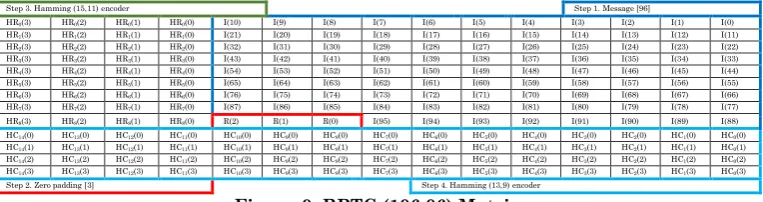
The Hamming (15,11) is encoded according to the above Hamming encode, I(0) to I(10) are a set of messages, HR0(0),
HR0(1), HR0(2), HR0(3), I(11) to I(21) derived from encoding are
a set of messages, HR1(0), HR1(1), HR1(2) and HR1(3) are
derived from encoding, till I(88) to R(2) are a set of messages, afterwards, Hamming (15,11) encoding is finished. After Hamming (15,11) encoding, the message array has changed to 15×9 form, and then Hamming (13,9) will be encoded.
Step 3. Hamming (15,11) encoder Step 1. Message [96]
HR0(3) HR0(2) HR0(1) HR0(0) I(10) I(9) I(8) I(7) I(6) I(5) I(4) I(3) I(2) I(1) I(0) HR1(3) HR1(2) HR1(1) HR1(0) I(21) I(20) I(19) I(18) I(17) I(16) I(15) I(14) I(13) I(12) I(11) HR2(3) HR2(2) HR2(1) HR2(0) I(32) I(31) I(30) I(29) I(28) I(27) I(26) I(25) I(24) I(23) I(22) HR3(3) HR3(2) HR3(1) HR3(0) I(43) I(42) I(41) I(40) I(39) I(38) I(37) I(36) I(35) I(34) I(33) HR4(3) HR4(2) HR4(1) HR4(0) I(54) I(53) I(52) I(51) I(50) I(49) I(48) I(47) I(46) I(45) I(44) HR5(3) HR5(2) HR5(1) HR5(0) I(65) I(64) I(63) I(62) I(61) I(60) I(59) I(58) I(57) I(56) I(55) HR6(3) HR6(2) HR6(1) HR6(0) I(76) I(75) I(74) I(73) I(72) I(71) I(70) I(69) I(68) I(67) I(66) HR7(3) HR7(2) HR7(1) HR7(0) I(87) I(86) I(85) I(84) I(83) I(82) I(81) I(80) I(79) I(78) I(77) HR8(3) HR8(2) HR8(1) HR8(0) R(2) R(1) R(0) I(95) I(94) I(93) I(92) I(91) I(90) I(89) I(88) HC14(0) HC13(0) HC12(0) HC11(0) HC10(0) HC9(0) HC8(0) HC7(0) HC6(0) HC5(0) HC4(0) HC3(0) HC2(0) HC1(0) HC0(0) HC14(1) HC13(1) HC12(1) HC11(1) HC10(1) HC9(1) HC8(1) HC7(1) HC6(1) HC5(1) HC4(1) HC3(1) HC2(1) HC1(1) HC0(1) HC14(2) HC13(2) HC12(2) HC11(2) HC10(2) HC9(2) HC8(2) HC7(2) HC6(2) HC5(2) HC4(2) HC3(2) HC2(2) HC1(2) HC0(2) HC14(3) HC13(3) HC12(3) HC11(3) HC10(3) HC9(3) HC8(3) HC7(3) HC6(3) HC5(3) HC4(3) HC3(3) HC2(3) HC1(3) HC0(3) Step 2. Zero padding [3] Step 4. Hamming (13,9) encoder
Figure 9: BPTC (196,96) Matrix
Encode Hamming (13,9), I(0), I(11), I( 22),…, I(88) are a set of messages, HC0(0), HC0(1), HC0(2), HC0(3) are derived from
encoding, I(1), I(12), I(23),…, I(89) are a set of messages, HC1(0), HC1(1), HC1(2) and HC1(3) are derived from encoding,
the rest can be deduced accordingly, till HR0(3), HR1(3),
HR2(3),…, HR8(3) are a set of messages, afterwards, Hamming
the BPTC using a new Soft Hamming Decoder
is completed, the matrix has changed to 15×13 form, and then the interleaving is carried out.
The messages received by the receiving terminal are in the form of 15×13 matrix, de-interleaving must be carried out before decoding to restore the original message sequence. Decoding can be carried out after de-interleaving, the decoding should be in such an order that encoded late should be decoded first, that encoded early should be decoded late.
Decode Hamming (13,9) according to the aforesaid Hamming decode, I(0), I(11), I( 22),…, HC0(2) and HC0(3) after
sequence restoration are a set of messages, decode and correct I(0), I(11), I(22),…, I(88), I(1), I(12), I(23),…, HC1(2) and HC1(3)
are a set of messages, decode and correct I(1), I(12), I(23),…, I(89), the rest can be deduced accordingly, till HR0(3), HR1(3),
HR2(3),…, HC14(2) and HC14(3) are a set of messages,
afterwards, Hamming (13, 9) decoding is finished. After Hamming (13,9) decoding, the message array has changed to 15×9 form, and then Hamming (15,11) will be decoded.
Decode Hamming (15,11), I(0), I(1), I(2),…, HR0(2) and
HR0(3) are a set of messages, decode and correct I(0), I(1), …,
I(10). I(11), I(12), I(13),…, HR1(2) and HR1(3) are a set of
messages, decode and correct I(11), I(12), …, I(21), the rest can be deduced accordingly, till I(88) to HR8(3) are a set of
messages, afterwards, Hamming (15, 11) decoding is finished.
5. SIMULATION RESULTS AND ANALYSIS
A key performance index to evaluate the capacity-approaching is the BER given a received SNR over an AWGN channel. We consider a received SNR from 0 to 9 dB and examine the BER, as shown in the performance figures presented previously, Fig. 2, 3, 4, and 7. The received signal to noise ratio is considered here as Eb/N0 where Eb is the received energy per bit, and N0 is
following figures. For the evaluation, all size of hamming code from code length 7 into 127 was compared together, and the value of coding rate of each product turbo code is considered when compared to a simple hamming code. The code chosen are the (15,11), (31,26), and (63,57)-Hamming code. And the turbo product code chosen are formed by two identical hamming code and they will be compared with the BPTC (196,96) which is formed by the (15,11)-Hamming code concatenated with the (13,9)-reduced Hamming code.
5.1. BPTC vs Simple Hamming code
Figure 10: Simple Hamming code vs. BPTC (Identical).
For the (15,11), (31,26), and (63,57)-Hamming codes, which give to each 11, 26, and 57 information bits 4, 5, and 6 additional parity bits, and has a coding rate of approximately 0.7, 0.8, and 0.9 respectively. The (15,11)2, (31,26)2, and (63,57)2 BPTC
the BPTC using a new Soft Hamming Decoder
BPTC using the soft decoder which corrects the duets bit error or the triplets bit error. the BPTC increases the gain of the simple hamming code soft decoded by respectively 0.5, 0.75, and 0.75 dB and the gain with the hard decoded to 1.5, 2, and 2 dB respectively at BER = 10-4.
5.2. BPTC Comparison
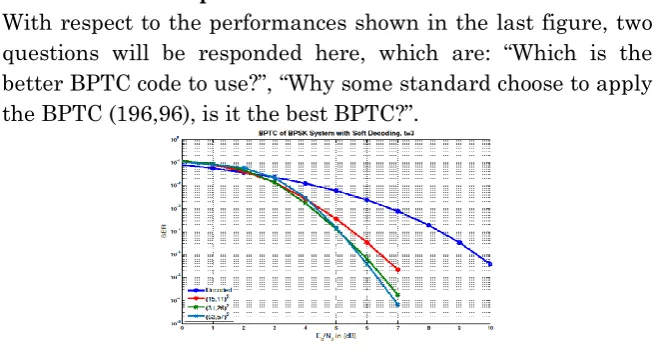
With respect to the performances shown in the last figure, two questions will be responded here, which are: “Which is the better BPTC code to use?”, “Why some standard choose to apply the BPTC (196,96), is it the best BPTC?”.
Figure 11: BPTC performances comparison.
Fig. 11 shows a comparison between the three cases presented before, where we remark directly that the (31,26)2 and the
(63,57)2 cases show the best performance, where the (31,26)2
BPTC, which has 0.7 as coding rate, slightly outperforms the (63,57)2 BPTC at low SNR (SNR<5 dB) and the (63,57)2 BPTC,
with coding rate equal to 0.8, has a very small gain with respect to the (31,26)2 BPTC code. We should not forget the coding rate
(15,11)-Hamming code and the second one the reduced (13,9)-Hamming code.
Figure 12: Comparison with the BPTC(196,96).
In the same time, Fig. 12 shows that the BPTC(225,121) formed by two identical (15,11)-Hamming code give approximately the same probability of error as the BPTC(196,96) with a coding rate slightly bigger. As we can see there are other BPTC that outperform the BPTC(196,96) with a coding rate bigger, much bigger. In despite that, the BPTC(196,96) still has the advantage of the block size, which is the smallest possible and these small block size could be necessary for some standards. So we recommend the BPTC(961,676) for standard with a bigger block size.
6. CONCLUSION
the BPTC using a new Soft Hamming Decoder
shows an obvious increase in efficiency, if we change the Hamming code used, but there is not one best edition for all the cases.
This paper observes the efficiency of BPTC, and compares the complexity and coding gain with Hamming code, and the physical mechanism of decoding efficiency difference between Hamming code and BPTC is discussed in the paper. This paper uses MatLab code for simulation in order to form a mathematical model of the system. The simulation results show that the soft decoding of the Hamming codes improves well the performance of the coding by more than 1 dB in some case. The BPTC scheme decoded hard doesn’t improve the performance with respect to the soft decoding of the simple Hamming code, but when our proposed soft decoder is used in the BPTC scheme, we obtained a gain of approximately 1 dB with respect to the soft decoding of the simple Hamming code. Finally, we have shown a good comparison between different Hamming code size and rate, and we have demonstrated that the (31,26)-Hamming code can be a good compromise when concatenated to give a BPTC(961,676) code when the block size is big. In the other hand, if the block size needed is small, the concatenation of the (15,11)-Hamming code and the (13,9)-Hamming code to give the BPTC(196,96) still the best compromise in despite of the loss in the coding rate.
In the future work, the results of simulations based on the modelling of the system will be compared with the real implementation of the system on a DSP chip to obtain a small software defined radio (SDR) system.
REFERENCES
2. [Berrou 1993] Berrou, C., Glavieux, A., and Thitimajshima, P., “Near Shannon Limit Error-Correcting Coding and Decoding: Turbo Codes,” IEEE Proceedings of the Int. Conf. on Communications, Geneva, Switzerland, May 1993 (ICC ’93), pp. 1064-1070.
3. [Divsalar 2001] Divsalar, D., Dolinar, S., and Pollara, F., “Iterative Turbo Decoder Analysis Based on Density Evolution,” IEEE Journal on Selected Areas in Communications, vol. 19, no. 5, pp. 891–907, May 2001. 4. [Divsalar 2004] Divsalar, D., Dolinar, S., “Concatenation of
Hamming Codes and Accumulator Codes with High-Order Modulations for High-Speed Decoding,” IPN Progress Report 42-156, February 15, 2004.
5. [Li 2004] Li, J, Narayanan, K. R. and Georghiades, C. N., "Product accumulate codes: a class of codes with near-capacity performance and low decoding complexity", IEEE Trans. Inform. Theory, vol. 50, pp. 31-46, 2004.
6. [Huang 2007] Huang, T. D.-H., Chang, C.-Y., Zheng, Y.-X., and Su, Y. T., “Product Codes and Parallel Concatenated Product Codes,” IEEE Wireless Communications and Networking Conference, March 2007 (WCNC 2007).
7. [Muller 2011] Muller, B., Holters, M., Zolzer, U., “Low Complexity Soft-Input Soft-Output Hamming Decoder,” IEEE proceedings of the 50th FITCE Congress, Palermo, Italy, September 2011 (FITCE 2011), pp. 242-246.
8. [Chen 2011] Chen, Y. H., Hsiao, J. H., Liu, P. F., Lin, K. F., "Simulation and Implementation of BPSK BPTC and MSK Golay Code in DSP Chips", Journal of Communications in Information Science and Management Engineering, CISME Vol. 1, No.4, Pages 46-54, 2011.
the BPTC using a new Soft Hamming Decoder