Double Beta Decay with a Segmented Enriched Germanium Detector.

(1)

ABSTRACT

LEVINER, LANCE EMORY. Double Beta Decay with a Segmented Enriched Germanium Detector. (Under the direction of Albert Young.)

Since the neutrino was first postulated to exist in 1930, it has been quite the challenge

to characterize this weakly interacting particle. It was not until 26 years later that the

neutrino was experimentally detected, and was not until the turn of the century that it

was determined neutrinos were massive particles. Which brings us to today, where many

properties of the neutrino are still unknown. Questions remain such as: what are the

absolute neutrino masses, is the mass hierarchy normal or inverted, and is the neutrino

its own antiparticle? Neutrinoless double beta-decay provides a means to potentially

address all three of these questions.

TheMajoranaexperiment is one of many experiments currently pursuing the

detec-tion of neutrinoless double beta-decay. The source used for the Majorana experiment

is76_{Ge, and the ultimate goal is to reach neutrinoless double beta-decay half-lives greater}

than 1027 years and absolute neutrino mass scales of 20-40 meV. To probe these regions

requires a tonne-scale experiment with a background count of less than one count per

tonne-year in the 4 keV region of interest (ROI) for 76_{Ge 0}_νββ _{decay of 2039 keV.}

In efforts to achieve such low background rates, the first segmented, n-type Ge

detec-tor, isotopically enriched to 85%76_{Ge was developed. This detector is based on the Ortec}

PT6x2 design and is referred to as SEGA (Segmented, Enriched Germanium Assembly).

The characterization of SEGA is presented, which includes: electric-field profile,

deple-tion voltage, leakage current, efficiency, calibradeple-tion, linearity, cross-talk, electronic noise,

resolution, and low-energy tailing. The detector’s segmentation and pulse shape analysis

(2)

(3)

Double Beta Decay with a Segmented Enriched Germanium Detector

by

Lance Emory Leviner

A dissertation submitted to the Graduate Faculty of North Carolina State University

in partial fulfillment of the requirements for the Degree of

Doctor of Philosophy

Physics

Raleigh, North Carolina

2014

APPROVED BY:

Paul Huffman David Haase

Chueng Ji Albert Young

(4)

DEDICATION

(5)

LIST OF TABLES

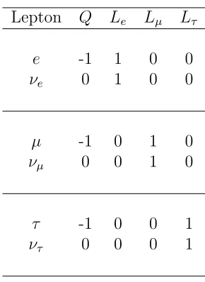
Table 1.1 Three leptonic doublets in the SM with their electron number (Le), muon number (Lµ), and tau number (Lτ) values listed. Le,Lµ, and

Lτ are conserved values in the Standard Model. . . 4

Table 1.2 Best fit values for neutrino oscillation parameters from [18]. The first and second rows for the parameters ∆m2 31, sin 2₍_θ 23), and sin2(θ13) correspond to the normal and inverted hierarchies respectively. . . 8

Table 2.1 Approximations for the impedance parameters in the transfer matrix T. . . 63

Table 3.1 Germanium isotopic abundances for the SEGA detector. . . 70

Table 4.1 Full-peak intensity parameters. . . 84

Table 4.2 γ-ray sources used for system linearity evaluation. . . 88

Table 4.3 Sources used for resolution study. . . 99

Table 4.4 Measured electronic noise and charge-collection contributions to the photopeak width along with the measured and projected FWHM values at 2039 keV for 6 µs rise time. The projected values as-sume 1.0 keV FWHM for the electronic noise contribution and the charge-collection contribution was calculated at 2039 keV. Errors are statistical uncertainties from Gaussian fits to the photopeaks and the errors from the extracted values for the W2 E parameter. . 102

Table 5.1 Retained fractions of events for simulated back-to-back 1020 keV electrons, as a function of position resolution (PR). . . 115

Table 5.2 Retained fractions of events for the double escape peak, 2040 keV full energy peak, 3060 keV full energy peak, and figure of merits, as a function of position resolution (PR), for the simulated HIγS runs. 117 Table 5.3 Retained fractions of events for the double escape peak, 2040 keV full energy peak, 3060 keV full energy peak, and figure of merits, as a function of position resolution (PR), for the “ideal” HIγS runs. . 118

Table 5.4 Retained fractions of events for the208_{Tl double escape peak,}228_Ac full energy (FE) peak,208_{Tl full energy peak, and figure of merits for} the simulated Thorium source, as a function of position resolution (PR). . . 119

Table 5.5 Simulated HIγS run results for segmentation and position resolution (PR) cuts applied to the entire detector. . . 121

(8)

Table 5.7 Simulated thorium source results for segmentation and position res-olution (PR) cuts applied to the entire detector. . . 122 Table 5.8 Sphericalγ-ray source results for segmentation and position

resolu-tion (PR) cuts applied to the entire detector. . . 122 Table 5.9 Retained fractions of events for double escape peak, 2040 keV full

energy peak, 3060 keV full energy peak, and figure of merits for HIγS pulse shape analysis on segment C2S1. The pulse shape parameter bins for this method were weighted by 1/γ1.5_{. . . .} ₁₂₉ Table 5.10 Retained fractions of events for double escape peak, 2040 keV full

energy peak, 3060 keV full energy peak, and figure of merits for HIγS pulse shape analysis on segment C2S1. The pulse shape parameter bins for this method were not weighted. . . 129 Table 5.11 Retained fractions of events for double escape peak, 2040 keV full

energy peak, 3060 keV full energy peak, and figure of merits for HIγS segmentation cut and pulse shape analysis for all segments. The pulse shape parameter bins for this method were weighted by 1/γ1.5_{. . . .} ₁₃₁ Table 5.12 Retained fractions of events for the 208Tl double escape peak,228Ac

full energy (FE) peak,208Tl full energy peak, and figure of merits for Thorium source data pulse shape analysis on segment C2S1. The pulse shape parameter bins for this method were weighted by 1/γ1.5_{. 136}

Table A.1 Integral cross-talk coefficients. . . 150 Table A.2 Electronic noise coefficients from ENC2 _versus _{rise-time curves. . .} ₁₅₁ Table A.3 Leakage current as measured across the feedback resistor with a

voltmeter and calculated from the h3 coefficient from the ENC2

versus rise-time curves. The feedback resistor and h3 coefficient

measurements were done in October, 2009 and December, 2009, respectively. . . 151 Table A.4 FWHM values for each physical segment at 1332 keV from the

Gaus-sian functional fits and modified GausGaus-sian functional fits. Also listed are the FWFM/FWHM ratios for the modified Gaussian functional fits, along with the integrated number of counts in the low-energy tail as a ratio to the number of counts in the photopeak. . . 153 Table A.5 The mean 10-90% rise-time values for events in the 60_{Co 1332 keV}

(9)

LIST OF FIGURES

Figure 1.1 Normal and inverted mass hierarchies for the three neutrino mass eigenstates. . . 9 Figure 1.2 Isobars for A=76. Single beta-decay is energetically forbidden to

intermediate nuclear states that are more weakly bound than the initial nuclear state. Transitions such as 76_Ge_→76_{Se can not occur} from successive beta-decays, but can through double beta-decay. . 15 Figure 1.3 Hypothetical spectrum of the kinetic energy of the two electrons

from double beta decay where the 0νββpeak a the end of the 2νββ spectrum is exaggerated for context. The 0νββ peak is broadened due to an assumed 2.5% energy resolution in the detector. . . 17 Figure 1.4 Feynman diagrams for two neutrino double beta-decay (left) and

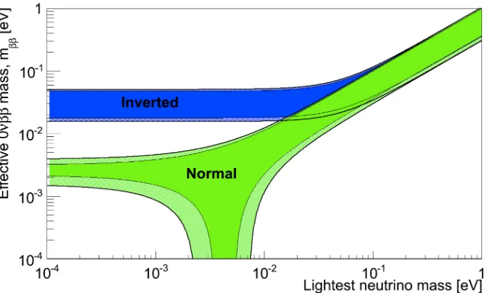
neutrinoless double beta-decay (right). . . 17 Figure 1.5 The effective Majorana neutrino mass as a function of the

light-est neutrino mass for both the normal and inverted cases. Figure generated using Eq. 1.43 and values from Table 1.2. Inner bands represent allowed regions using best-fit values for the normal and inverted cases. Encompassing bands represent experimental uncer-tainties. . . 20 Figure 1.6 Cross-sectional view of a _{Majorana Demonstrator} cryostat

where strings of detectors, shown in cyan, are suspended from a coldplate. . . 24 Figure 1.7 Cross-section view of the_{Majorana Demonstrator}with

shield-ing in place and one cryostat in the removed position. . . 25 Figure 1.8 The effective neutrino mass and half-life sensitivity as a function of

exposure in tonne-years for a76Ge 0νββ decay experiment. Curves are shown for background rates of 0, 0.1, 1, and 10 counts per tonne-year in the 4 keV ROI. The half-life conversion was achieved using Eq. 1.42 with G0ν and M0ν values from [57] and [58] respectively. Figure from [59]. . . 26

(10)

Figure 2.2 γ-ray attenuation as a function ofγ-ray energy for germanium. To-tal attenuation is presented along with the individual attenuation contributions from photoelectric absorption, Compton scattering, and pair production. One can see photoelectric absorption is over-come by Compton scattering around 140 keV, which eventually succeeds to pair production around 8 MeV. This figure was gen-erated using data from the NIST photon cross section database

[71]. . . 36

Figure 2.3 Representation of conduction and valence bands with donor and acceptor energy levels present in the band-gap. . . 41

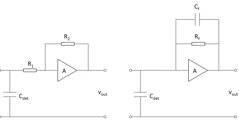
Figure 2.4 Simplified schematics of voltage and charge sensitive preamplifiers. 46 Figure 2.5 Simplified schematic of a detector-charge-sensitive preamplifier sys-tem. . . 49

Figure 2.6 Equivalent circuit for the detector-preamplier system presented in Fig. 2.5 with the parallel and series voltage sources represented by di2_p and dv2_s respectively [74]. isignal represents the detector signal current. . . 52

Figure 2.7 Miller equivalent circuit for Fig. 2.6 [74]. . . 52

Figure 2.8 Basic schematic for a CR differentiator. . . 54

Figure 2.9 Basic schematic for a RC integrator. . . 56

Figure 2.10 Representation of a two-fold segmented detector. The bias voltage is connected to the central electrode while the two outer segments are grounded. The charge sensitive preamplifiers are AC and DC coupled for the core and outer channels respectively. . . 61

Figure 2.11 Miller equivalent representation of Fig. 2.10. . . 62

Figure 3.1 The SEGA detector’s germanium crystal with indium pads for the contacts. . . 69

Figure 3.2 The ORTEC PT6x2 detector geometry. The SEGA detector is not “bulletized”, which means there is no radius for the closed-end, outer edge. . . 71

Figure 3.3 Photographs of components of the SEGA detector as they are as-sembled inside of the temporary cryostat. . . 73

(11)

Figure 4.2 Counts in the60_{Co 1332 keV}_γ_{-ray peak (for the C1 and C2} chan-nels connected together) as a function of bias voltage. The slope of the efficiency curve approaches zero as the operating voltage is reached, confirming that effectively all charge deposited in the detector is collected. . . 79 Figure 4.3 Leakage current from segments S1 to S6 as a function of bias applied

to C1 and C2. These measurements were done in February, 2003. 81 Figure 4.4 Decay scheme for60_{Co. . . .} ₈₃ Figure 4.5 SEGA detector geometry used in MaGe simulation. The cold finger

and some small parts were not simulated. . . 86 Figure 4.6 Energy response of C2 channel for C2S2 events from a60_{Co source}

and various background sources, along with the residuals of the data-points from the linear fit. . . 88 Figure 4.7 Cross-talk band in C1 for C2S2 events. . . 90 Figure 4.8 Superpulses (ADC valuesversustime) from each preamplifier

chan-nel for 60Co 1332 keV γ-ray events in segment C2S3. C2 and S3 show a clear integrated charge from an event, while the overall non-zero integrated charge in channels C1, S1, S2, S4, S5, and S6 indicate cross-talk between channels. The induced pulses with zero integrated charge are called mirror pulses. . . 92 Figure 4.9 Total energy determined by summing the outer S channels (S1-S6)

energies before (top) and after (bottom) the cross-talk correction was applied for multiplicities 1, 2, and 3. . . 94 Figure 4.10 FWHM and mean photopeak values for the 1332 keV, 60_Co

pho-topeak as a function of multiplicity. The summed center contact channels (C1 and C2) values are presented in column one with the summed S channels (S1-S6) values in column two. . . 95 Figure 4.11 For each readout contact, we depict ENC2 versus rise-time curves

along with the fitted contributions for white series noise (x−1_term), white parallel noise (xterm), and non-white noise (constant term) (see coded legend at right of figure; noise components are repre-sented by dashed/dotted lines with exception to S2 being solid). The peaking time for a trapezoidal filter shaping network is its rise-time [76]. . . 97 Figure 4.12 σ2 _versus _{energy for Gaussian fits to the full-energy peak for all}

(12)

Figure 4.13 σ2_versus_{energy for Gaussian fits to the full-energy peak for summed} inner contacts (C1 and C2) and summed outer contacts (S1-S6). Allσ2 values were given a 5% uncertainty. . . 103 Figure 4.14 1332 keV photopeak for channel S1 with S1C1 and S1C2

single-segment cuts. The degree of low-energy tailing is clearly greater in the C1 segment where the low-field regions are present. The width of the fit band reflects uncertainties of the fits to the low-energy tail.105

Figure 5.1 The High Intensity γ-ray Source at the Duke Free Electron Laser Laboratory (DFELL). . . 110 Figure 5.2 Top view of the HIγSγ vault. . . 112 Figure 5.3 HIγS beam path through the SEGA detector and cryostat. . . 113 Figure 5.4 Simulated 3060 keV HIγS run results for various position resolution

cuts following a segmentation cut for segment C2S1. . . 116 Figure 5.5 Simulated 2040 keV HIγS run results for various position resolution

cuts following a segmentation cut for segment C2S1. . . 116 Figure 5.6 Simulated 3060 keV HIγS run results for segmentation and position

resolution cuts applied to the entire detector. . . 120 Figure 5.7 Simulated 2040 keV HIγS run results for segmentation and position

resolution cuts applied to the entire detector. . . 121 Figure 5.8 Pulse shape analysis phase space parameters from cuts on the

dou-ble escape peak (blue dotted line) and full-energy peak (green solid line) for the 3060 keV run (risetime is in units of ns). . . 125 Figure 5.9 Risetime [ns] vs. asymmetry for cuts on the double escape peak

(left) and full-energy peak (right) for the 3060 keV run. . . 126 Figure 5.10 Risetime [ns] vs. moment for cuts on the double escape peak (left)

and full-energy peak (right) for the 3060 keV run. . . 126 Figure 5.11 Three dimensional phase space for cuts on the double escape peak

(left) and full-energy peak (right) for the 3060 keV run (risetime is in units of ns). . . 127 Figure 5.12 3060 keV HIγS run results for a PSA cut following a segmentation

cut for segment C2S1. . . 128 Figure 5.13 2040 keV HIγS run results for a PSA cut following a segmentation

cut for segment C2S1. . . 128 Figure 5.14 3060 keV HIγS run results for segmentation and PSA cuts applied

to the entire detector. . . 130 Figure 5.15 2040 keV HIγS run results for segmentation and PSA cuts applied

to the entire detector. . . 131 Figure 5.16 Comparison of 3060 keV HIγS run experimental data with

(13)

Figure 5.17 Pulse shape analysis phase space parameters from cuts on the dou-ble escape peak (blue dotted line) and full-energy peak (green solid line) from the208Tlγ-ray in the Th decay chain (risetime is in units of ns). . . 133 Figure 5.18 Risetime [ns] vs. asymmetry for cuts on the double escape peak

(left) and full-energy peak (right) from the 208Tl γ-ray in the Th decay chain. . . 134 Figure 5.19 Risetime [ns] vs. moment for cuts on the double escape peak (left)

and full-energy peak (right) from the 208Tl γ-ray in the Th decay chain. . . 134 Figure 5.20 Three dimensional phase space for cuts on the double escape peak

(left) and full-energy peak (right) from the 208Tl γ-ray in the Th decay chain (risetime is in units of ns). . . 135 Figure 5.21 Th source data results for a PSA cut following a segmentation cut

(14)

Chapter 1 Introduction

The basis of this dissertation is the study of the first segmented, n-type Ge detector,

isotopically enriched to 85% 76_{Ge, and its application to double beta-decay experiments.}

This detector, based on the Ortec PT6x2 design and referred to as SEGA (Segmented,

Enriched Germanium Assembly), was developed as a possible prototype for neutrinoless

double beta-decay (0νββ) measurements by theMajoranacollaboration. This chapter

will serve as a primer for the neutrino physics related to the _Majorana experiment,

as well as provide an overview of the _Majorana experiment and the motivation for

segmented detectors.

1.1 Neutrinos

1.1.1 A Brief History

The existence of the neutrino was first postulated in 1930 by Wolfgang Pauli to explain

(15)

gamma decay in that it was a two body decay, as shown in Eqs. (1.1) and (1.2),

X(A, Z)→X0(A, Z + 1) +e− (1.1)

X(A, Z)→X0(A, Z−1) +e+ (1.2)

whereX(A, Z) is the mother nucleus,X0(A, Z±1) is the daughter nucleus, and eis the beta particle (either the electron (e−) for β− decay or the positron (e+_{) for} _β+ _decay).

It is straightforward to show that due to conservation of energy and momentum this

two-body decay should produce a mono-energetic beta particle. However, observation

showed that the beta particle from the decay had a continuous energy spectrum ranging

from zero to the transition energy of the decay. In addition to violation of conservation

of energy and momentum, this process seemed to imply that the spin of the daughter

nucleus in the decay was off by a factor of 1/2 compared to the value suggested by

Rutherford.

In efforts to explain this result, several theories were proposed, including the

propo-sition by Niels Bohr of modifying the conservation of energy laws, but it was Pauli’s

suggestion of a second particle’s presence that eventually proved to prevail. The particle

Pauli predicted was proposed to be electrically neutral by conservation of charge, have

a spin of 1/2 by conservation of angular momentum, have a mass comparable to that

of the electron, and be “weakly” interacting with ordinary matter because the detectors

failed to record its energy. To keep up with the nomenclature at the time, Pauli

sug-gested naming the particle the “neutron”, but the term “neutron” was later used for the

more massive particle discovered by James Chadwick in 1932. Enrico Fermi later termed

(16)

decay and also suggested the possibility that neutrinos were massless [1].

The theoretical evidence for the neutrino continued to solidify, but the direct detection

of the particle itself proved to be challenging due to the particle’s “weakly” interacting

nature with ordinary matter. It wasn’t until 1956 that there was experimental evidence

for the detection of the neutrino by Cowan and Reines at the Savannah River nuclear

reactor in South Carolina [2, 3]. The method of detection was through observation of the

inverse beta-decay process,

ν+p→n+e+ (1.3)

where ν is the anti-neutrino, p is the proton, n is the neutron, and e+ _{the positron.}

Cowan and Reines used the anti-neutrino flux from a nuclear reactor, approximately

5×1013_/_cm2_{s, incident upon a large water tank, and detected the positron from the}

reaction by looking for the annihilation γ-rays using scintillators and photomultiplier

tubes.

In the Standard Model (SM), which is based on an SU(2)×U(1) gauge model [4],

neutrinos are massless, neutral leptons that pair with a charged lepton to form a leptonic

doublet. There are three leptonic doublets in the SM and they are classified by their

flavor as electron (e), muon (µ), or tau (τ) to form the three generations or families

shown in Table 1.1. In 1953, Konopinski and Mahmoud formulated the concept of lepton

number, L, with the six leptons in Table 1.1 being assigned a value of L = 1 and their

antiparticles having a value of L = −1 [5]. In the SM, lepton number is conserved and

no evidence to suggest otherwise has been discovered. Also, due to the structure of the

V −A theory [6, 7, 8], all neutrinos in the SM are left-handed, while all antineutrinos

(17)

Table 1.1: Three leptonic doublets in the SM with their electron number (Le), muon number (Lµ), and tau number (Lτ) values listed. Le, Lµ, andLτ are conserved values in the Standard Model.

Lepton Q Le Lµ Lτ

e -1 1 0 0

νe 0 1 0 0

µ -1 0 1 0

νµ 0 0 1 0

τ -1 0 0 1

ντ 0 0 0 1

1.1.2 Massive Neutrinos

The neutrino’s mass is one of the more fascinating properties of the neutrino. In the

Standard Model, neutrinos are massless particles. However, with the confirmation, at

the beginning of the century, that neutrinos oscillate in flavor and are therefore massive

particles, the first extension of the Standard Model since its inception became a generally

accepted fact.

Neutrino Oscillations

Motivated by the phenomenon of strangeness oscillations in K mesons [9], in 1957

tecorvo proposed the idea that neutrinos could oscillate [10, 11]. At the time of

Pon-tecorvo’s proposition, the only known neutrino was the electron neutrino, and in order to

(18)

neutrino [12], which is a neutrino that does not participate in weak interations. With

the discovery of the muon neutrino in 1962 [13], it became apparent that the neutrino

oscillations could be due to the mixture of flavor and mass eigenstates. The standard

theory of neutrino oscillations was developed in 1975-1976 by Eliezer and Swift, Fritzsch

and Minkowski, and Bilenky and Pontecorvo [14, 15, 16, 17]. A brief overview is

pre-sented below of this standard theory and how the transition probabilities are related to

the mass squared differences of the mass eigenstates.

Initially, neutrinos in flavor eigenstates, |ναiwhere (α=e, µ, τ), are created through

charged-current (CC) interaction processes1 _{whose interaction Lagrangian is expressed}

as [4]

L(_I,LCC) =− g

2√2

j_W,Lρ Wρ+jρ † W,LW

† ρ

, (1.4)

where j_W,Lρ is the charged leptonic current given by

j_W,Lρ = 2X α

ναLγρ`αL. (1.5)

Expressing these flavor eigenstates as linear combinations of massive neutrino eigenstates,

|νki, as follows

|ναi=

X

k

U_αk∗ |νki, (1.6)

whereU_αk∗ are coefficients of the Portecorvo-Maki-Nakagawa-Sakata (PMNS) mixing

ma-trix (similar to the CKM unitary mixing mama-trix for quarks), it is possible to determine

the time evolution of the flavor eigenstates using the Schr¨odinger equation

id

dt |vk(t)i=H |vk(t)i. (1.7)

(19)

gen-The eigenvalues of the Hamiltonian in Eq. (1.7) are given by

H |νki=Ek |νki, (1.8)

where

Ek=

q

p2₊_m2

k, (1.9)

and the solution to the Schr¨odinger equation is the well known plane wave solution

|να(t)i=

X

k

U_αk∗ e−iEkt_|_ν

ki. (1.10)

Expressing the mass eigenstates as linear combinations of the flavor eigenstates as

|νki=

X

α

Uαk |ναi (1.11)

and substituting Eq. (1.11) into Eq. (1.10) gives

|να(t)i=

X

β=e,µ,τ

X

k

U_αk∗ e−iEkt_U

βk

!

|νβi. (1.12)

To determine the transition probability Pνα→νβ(t) one simply takes the absolute square

of the amplitude of να →νβ, which gives

Pνα→νβ(t) =

X

k,j

U_αk∗ UβkUαjUβj∗ e

−i(Ek−Ej)t_. _(1.13)

Using the ultrarelativistic approximation for the neutrino’s energy given by

Ek'E+

m2_k

(20)

and substituting

Ek−Ej ' ∆m2

kj

2E , (1.15)

where ∆m2

kj =m2k−m2j, into Eq. (1.13) the transition probability can be expressed in terms of the squared differences of the neutrino mass eigenstates as follows

Pνα→νβ(t) =

X

k,j

U_αk∗ UβkUαjUβj∗ e −i∆m

2 kjt 2E

!

. (1.16)

Assuming only three flavors of neutrinos exist, the PMNS matrix can be expressed as

follows [4] U =      

1 0 0

0 c23 s23

0 −s23 c23

           

c13 0 s13e−iδ

0 1 0

−s13eiδ 0 c13

           

c12 s12 0

−s12 c12 0

0 0 1

           

e−iα21 0 0

0 e−iα22 0

0 0 1

      , (1.17)

where sij and cij being the sines and cosines of the mixing angles, δ the Dirac CP

violating phase, and αi the (possible) Majorana phases. It is important to note, from

Eq. (1.16), only information concerning the mass squared differences, mixing angles

and CP violating phase values of the PMNS matrix are possibly available from neutrino

oscillation experiments. The best fit values for these parameters are listed in Table 1.2

with the exception of the CP violating phase, which has proven difficult to measure as

a result of the smallness of the θ13 value. In order to investigate the absolute neutrino

mass scale, mass hierarchy of the mass eigenstates, or Majorana nature of the neutrino,

(21)

Table 1.2: Best fit values for neutrino oscillation parameters from [18]. The first and second rows for the parameters ∆m2₃₁, sin2(θ23), and sin2(θ13) correspond to the normal and inverted hierarchies respectively.

Parameter Best fit value ±1σ

∆m2

21(10−5eV2) 7.59+0−0..2018

∆m2 31(10

−3_eV2₎ ₂_.₄₅_±₀_.₀₉

−(2.34+0₋₀._.10₀₉)

sin2(θ12) 0.312+0−0..017015

sin2(θ23) 0.51±0.06 0.52±0.06

(22)

Figure 1.1: Normal and inverted mass hierarchies for the three neutrino mass eigenstates.

Majorana and Dirac Neutrinos

As stated in Sec. 1.1.2, neutrinos in the Standard Model are massless and right-handed

neutrinos do not exist. However, due to the confirmation of neutrino oscillations, it is

now known that neutrinos are indeed massive particles and understanding how neutrinos

acquire mass has required the establishment of a new Standard Model.

The simplest extension to the Standard Model that allows massive neutrinos to exist

is the introduction of right-handed neutrinos. To show how this is so, one can be begin

with the Dirac Lagrangian

(23)

Using the chirality matrixγ5_{, defined in terms of the Dirac matrices by Eq. (1.19),}

γ5 =γ5 =iγ0γ1γ2γ3, (1.19)

and having the eigenvalues +1 and -1, it is possible to express the generic fermion field

ψ in terms of the chirality eigenfunctions ψR and ψL, which are referred to as the

right-handed and left-right-handed chiral fields respectively, as

ψ =ψR+ψL, (1.20)

where

ψR =

1 +γ5

2 ψ, (1.21)

ψL=

1−γ5

2 ψ. (1.22)

Substituting Eq. (1.20) into Eq. (1.18) and using the properties of the chirality projection

matrices defined by,

PR=

1 +γ5

2 (1.23)

and

PL =

1−γ5

2 , (1.24)

one can show the Lagrangian becomes

L=ψRi ←→

∂ ψR+ψLi ←→

∂ ψL−m(ψRψL+ψLψR). (1.25)

From Eq. (1.25) one can see that the mass term in Lagrangian couples the right-handed

(24)

By Euler-Lagrange methods it can be shown that the equations of motion for the

chiral fields are coupled by the mass term and are given by

iγµ∂µψL =mψR (1.26)

and

iγµ∂µψR=mψL. (1.27)

Only when the fermion is massless do the equations of motion become independent and

the particle can be described by a two-component spinor.

Another possible theory that accommodates the existence of massive neutrinos is one

proposed by Majorana in 1937 [19] that involves the possibility of a particle being its

own antiparticle. These particles are referred to as Majorana particles, whereas particles

who are not their own antiparticles are referred to as Dirac particles. Typically massive

fermions are described by a four-component Dirac spinor whose right-handed and

left-handed chiral fields are coupled as shown in Eq. (1.25). Majorana proposed that it is

possible to describe a massive particle with only a two-component spinor. To do so,

Majorana had to find a condition for which the equations of motion given in Eqs. (1.26)

and (1.27) where equal. This is accomplished by the Majorana condition

ψ =ψL+ψR =ψL+CψL T

, (1.28)

which can be simply written as

ψ =ψC. (1.29)

(25)

that Majorana mass terms appear as follows

LL mass =

1

2mL(ψL C

ψL+ψLψLC), (1.30)

LR mass =

1

2mR(ψR C

ψR+ψRψRC). (1.31)

In summary, from Eqs. (1.25), (1.30), and (1.31) it is only possible for the neutrino to

be a massive Dirac particle if the chiral fieldψRexists, and if so the neutrino Lagrangian

will contain a Dirac mass term given by

LD

mass=mD(ψRψL+ψLψR). (1.32)

However, if the neutrino is a Majorana particle, it is possible for the neutrino Lagrangian

to also contain the Majorana mass terms given by Eqs. (1.30) and (1.31), with the

existence of the chiral field ψR not being a requirement for the neutrino to be a massive

particle.

The most general neutrino Lagrangian mass term is a Dirac-Majorana mass term

given by

LD+M mass =L

D

mass+L L

mass+L R

mass, (1.33)

which can be written elegantly in matrix form as

LD_mass+M = 1 2N

T LC

†_M

(26)

where NL is a column matrix of the left-handed fields given by,

NL =



 

νL

νC R





, (1.35)

Mis a symmetric mass matrix given by

M=



 

mL mD

mD mR





, (1.36)

and h.c. is the Hermitian conjugate. To find the massive neutrino eigenstates and the

mass eigenvalues, one must diagonalize the mass matrix M, which can be done by a

unitary transformation of the chiral fields.

It should also be noted that if the Majorana particle is discovered it would

demon-strate that Lepton number is not conserved. Although the phenomenon of Lepton number

violation is expected in the Standard Model through B-L conserving excitations referred

to as “sphalerons”, it is not possible at present to observe the SM-predicted effects.

Hence, observation of L violation will involve new, beyond-Standard-Model (BSM)

ef-fects.

1.2 Neutrinoless Double Beta-Decay

Although the question of whether neutrinos are massive particles has been answered

by neutrino oscillations, there are still many properties of the neutrino left unanswered

including:

(27)

2. Is the mass hierarchy normal or inverted?

3. Is the neutrino its own antiparticle?

While aspects 1 and 2 can possibly be addressed through other avenues such as

neu-trino oscillation experiments, beta decay endpoint measurements, or cosmology, the most

promising method of addressing all 3 is through neutrinoless double beta-decay.

Neutrinoless double beta-decay (0νββ) is a unique process that is not allowed in the

Standard Model. It is analogous to two neutrino double beta-decay (2νββ), which is

allowed, so both will be discussed here. Two neutrino double beta-decay, first proposed

in 1935 by Goeppert-Mayer [20], is a second order weak process described by

X(A, Z)→X0(A, Z + 2) + 2e−+ 2νe (2β2−ν) (1.37)

and

X(A, Z)→X0(A, Z−2) + 2e++ 2νe (2β2+ν). (1.38)

The decay rate can be expressed as

(T2ν 1/2)

−1

=G2ν(Qββ, Z)|M2ν |2, (1.39)

where G2ν(Qββ, Z) is a phase space factor and M2ν are nuclear matrix elements. From

Eqs. (1.37) and (1.38) one can see that the energy from the 2νββdecay is shared between

the four new particles and the total kinetic energy of the electrons (positrons) for 2β₂−_ν

(2β₂+_ν) decay is a continuous distribution from zero up to near theQvalue of the process.

In order for double beta-decay to be allowed, the final nuclear state has to be more

(28)

one must consider other factors. Since two neutrino double beta-decay is a second order

weak process it is much easier for the isotope to decay through other modes if the first

order weak process is allowed. So for the two neutrino double beta-decay process to

be observable, the transmission to the intermediate nuclear state with Z ±1 must be

forbidden or suppressed, as shown in Fig. 1.2. Typically double beta-decay only occurs

between even-even nuclei as the pairing force between identical nucleons increases the

binding energy of the isotope.

Thirty-five naturally occurring isotopes are capable of undergoing 2β₂−_ν decay and the

process has been measured in eleven [21]. However, the 2β₂+_ν decay process is more scarce

as it is only allowed in six naturally occurring isotopes [22]. A prominent reason why

the 2β₂+_ν decay process is so much more rare than the 2β₂−_ν decay process is because of

(29)

electron capture. If the intermediate state’s ground state energy is not greater than the

initial state’s ground state energy plus the rest mass of the electron, then the electron

capture process is allowed. Of the six 2β₂+_ν candidates, only one has a Q value greater

than 1 MeV, while of the thirty-five 2β₂−_ν candidates, eleven have Q values greater than

2 MeV. Since the decay rate increases greatly with Q [23], the 2β₂+_ν decays are much

harder to observe and are studied less.

Neutrinoless double beta-decay was suggested by Furry in 1939 [24] and can be

de-scribed by

X(A, Z)→X0(A, Z+ 2) + 2e− (2β₀−_ν) (1.40)

and

X(A, Z)→X0(A, Z −2) + 2e+ (2β₀+_ν). (1.41)

Neutrinoless double beta-decay is not an allowed process in the SM as it requires a

violation of lepton number by 2 (∆L = 2). The sum of the kinetic energies of the two

electrons (positrons) for 2β₀−_ν (2β₀+_ν) must equal (up to recoil order corrections for energy

carried away by the daughter nucleus) the Q value of the decay. This means the 2νββ

and 0νββ can be distinguished from one another by measuring the energy spectrum of

the electrons emitted in the decay as shown in Fig. 1.3.

The Feynman diagrams depicting both two neutrino and neutrinoless double

(30)

β β

E/Q

0 0.2 0.4 0.6 0.8 1

Counts (arbitrary)

0 0.2 0.4 0.6 0.8 1

β β ν

0

β β ν

2

Figure 1.3: Hypothetical spectrum of the kinetic energy of the two electrons from double beta decay where the 0νββ peak a the end of the 2νββ spectrum is exaggerated for context. The 0νββ peak is broadened due to an assumed 2.5% energy resolution in the detector.

(31)

There are many suggested theories for the lepton number violating mechanism

respon-sible for 0νββ decay including: the existence of right-handed weak currents [25], heavy

Majorana neutrinos [26], leptoquarks [27], and SUSY particles [28]. However, all models

require the neutrino to be a Majorana particle, so low mass Majorana neutrinos provide

the simplest mechanism for this process, and can be considered the scenario providing

the motivation for current experiments.

Assuming low mass Majorana neutrinos to be the mediators for 0νββ, the decay rate

can be expressed as

(T0ν 1/2)

−1 ₌_G

0ν(Qββ, Z)|M0ν |2 hmββi2, (1.42)

where G0ν(Qββ, Z) is a phase space factor, M0ν are nuclear matrix elements, andhmββi

is the effective Majorana mass of the electron neutrino given by

hmββi2 =

X i

U_ei2mi

2

=U_e2₁m₁ +U_e2₂m₂eα2−α1 +U_e2₃m₃e−α1−2σ

2

. (1.43)

Eq. 1.42 can be written more generally to account for all possible lepton number violating

mechanisms as

(T0ν 1/2)

−1 ₌_G

0ν(Qββ, Z)|M0νη|2, (1.44)

where η contains all of the lepton number violation information, and both M0ν and η

depend on the 0νββ mechanism.

For neutrinoless double-beta decay experiments, the observable is the decay rate

given by Eq. 1.42 or Eq. 1.44. The ability to extract the underlying physics for the 0νββ

process inherently depends upon one’s ability to determine the parameters governing

the decay rate. The phase space factor G0ν(Qββ, Z) can be reliably determined with

(32)

main methods for calculating the nuclear matrix elements are the Quasi-particle Random

Phase Approximation (QRPA) and the Nuclear Shell Model (NSM), where differences

between the two methods include the number of particles used and how the correlations

are constrained. Recent publications show the deviations in the nuclear matrix element

values calculated between the two models are improving, but still differ by roughly a

factor of two [58, 30]. Additional methods for determining the nuclear matrix elements

include the Interacting Boson Model (IBM-2) [31], Projected Hartree-Fock-Boboliubov

(PHFB) [32], and Energy Density Functional methods [33].

If the 0νββdecay process is observed, it would imply neutrinos are Majorana particles

[34] and lepton number is not conserved. Eq. 1.42 shows that it is also possible to

extract an effective Majorana neutrino mass term given by Eq. 1.43. From the effective

Majorana mass term, it is possible to investigate the absolute neutrino mass scale as

shown in Fig. 1.5 where the effective Majorana mass, hmββi, is shown as a function of

the lightest neutrino mass. Depending upon if the electron neutrino is dominated by

the lightest neutrino mass eigenstate or not, the mass hierarchy is referred as normal or

(33)

Figure 1.5: The effective Majorana neutrino mass as a function of the lightest neutrino mass for both the normal and inverted cases. Figure generated using Eq. 1.43 and values from Table 1.2. Inner bands represent allowed regions using best-fit values for the normal and inverted cases. Encompassing bands represent experimental uncertainties.

It is possible that some cancellation occurs within the Majorana mass term due to the

CP phases. To better understand the physics, it is helpful to have complimentary mass

measurements to constrain the parameters. With beta-decay endpoint measurements,

the measured mass term is given by

hmβi2 =

X

i |Uei|

2

m2_i, (1.45)

which is independent of the CP phases and only depends upon the absolute square values

of the PMNS matrix. The current best measurements ofhmβiare given by the Mainz [35]

and Troitzk [36] tritium beta-decay endpoint measurements, which place upper bounds

(34)

KATRIN experiment plans to improve upon this measurement and approach sensitivities

of mβ .200 meV [37]. Another constraint imposed on the mass terms by cosmological

models that determine the appropriate contribution of neutrinos to the energy density

of the universe, which is sensitive to the sum of the neutrino masses, is given by

mcosmo_ν =X i

mi. (1.46)

Although the results are dependent upon the model and data used, the current model

independent upper limit for the sum of the neutrino masses can be approximated as

mcosmo

ν .1 eV [38, 39].

Experimentally observing double beta-decay processes can be achieved through three

different methods: geochemical, radiochemical, and direct. Both geochemical and

ra-diochemical methods detect the decay by observing the daughter only, meaning there is

no way to differentiate between the 2νββ and 0νββ decay modes. The direct method

observes the decay by measuring the energies of the emerging electrons and therefore

has the ability to distinguish between the two decay modes. For this reason, discussion

in this body of work will be limited to the direct method of detection and for a more

comprehensive review of all three methods see references [22] and [40].

The limit of a neutrinoless double beta-decay experiment’s sensitivity to the effective

neutrino mass can be written as [41]

hmββi= 2.50×10−8eV

W f xG0ν_|_M

0ν|2

1/2

b∆E M T

1/4

, (1.47)

where W is the molecular weight of the source material, f is isotopic abundance, x

(35)

background counts per kg·yr·keV, ∆E is the energy region of interest for 0νββ decay,

M is the isotopic mass in kg, T is the live time of the experiment, and (G0ν _and _M

0ν)

carry the same definition as in Eq. 1.42. From Eq. 1.47, a few apparent requirements

to reach physically relevant neutrino mass sensitivities are a massive source, minimal

backgrounds, and excellent detector technology. The factor of source material mass

is a somewhat scalable parameter, but the other two requirements can be logistically

addressed in different ways.

As one can see, the minimization of backgrounds is critical for double beta-decay

experiments. The prominent background sources in 0νββ decay experiments result from

natural radioactivity in materials, cosmogenic sources and ingrowth, and 2νββ decay

[42]. It is common in all materials that there is some presence of radioactive elements

such as uranium and thorium, whose decay chains have several decays that are capable

of depositing enough energy within the detector active volume to overlap with the

en-ergy range of interest for 0νββ decay. The reduction of these elements through use of

ultra-clean materials and sophisticated purification schemes is reaching new frontiers. To

reduce the cosmogenic backgrounds it is common for low-background experiments to

func-tion deep underground. In fact, the producfunc-tion and storage of experimental components

underground has become necessary for some experiments to minimize the magnitude of

cosmogenic ingrowth of radioactive sources. The extent for which the 2νββ decay

spec-trum can contaminate a 0νββ decay measurement is quite clear in an approximation of

the 0νββ signal to 2νββ background ratio given by [43]

S

B =

me 7Qδ6

Γ0ν Γ2ν

= me

7Qδ6 T2ν

1/2

T0ν

1/2

(36)

where me is the electron mass and δ is the detector energy resolution (FWHM) at the

0νββdecayQvalue. Eq. 1.48 demonstrates why one would desire detectors with excellent

energy resolution in 0νββ decay experiments.

1.3 The Majorana Experiment

The Majorana experiment is predominately focused on the search for 0νββ of 76Ge

[44, 45, 46]. The observation of neutrinoless double beta-decay would establish that

neutrinos are Majorana particles, show that lepton number is not conserved, and provide

information concerning the absolute neutrino mass scale [42, 48, 49]. The ultimate goal

of the Majorana experiment is to probe 0νββ half-lives greater than 1027 years and

the absolute neutrino mass scale at 20-40 meV. To do so would require a tonne-scale

experiment with a background count of less than one count per tonne-year in the 4 keV

region of interest (ROI) for76_{Ge 0}_νββ _{decay of 2039 keV.}

Prior to development of a tonne-scale experiment, the Majorana collaboration is

currently constructing the Majorana Demonstrator [50] at the 4850’ level of the

Sanford Underground Research Facility (SURF), formerly Homestake Mine, in Lead,

SD. The Demonstrator will be composed of approximately 40 kg of p-type point

contact (PPC) [51, 52] high purity germanium (HPGe) detectors for which up to 30 kg

will be enriched to 86% 76_{Ge. Each detector used in the}

Demonstrator will have a

mass of approximately 0.6-1.0 kg. These crystals will be assembled in a stacked geometry

to form a string of detectors, with each string composed of three to five crystals. A total

of seven strings are attached to an electro-formed copper coldplate and positioned inside

(37)

Figure 1.6: Cross-sectional view of a Majorana Demonstrator cryostat where

strings of detectors, shown in cyan, are suspended from a coldplate.

The_Demonstratorwill consist of two cryostats positioned inside active and passive

layers of shielding, for background suppression, as shown in Fig. 1.7. The first layer

outside of the cryostats is a 5 cm thick layer of electro-formed copper, followed by a 5 cm

thick layer of oxygen-free high-conductivity (OFHC) copper, a 45 thick cm layer of lead,

a radon exclusion box, an active scintillator veto, and a 30 cm thick layer of polyethylene.

The detectors are cooled using a thermosyphon that is routed from the cryostats, outside

(38)

Figure 1.7: Cross-section view of the Majorana Demonstrator with shielding in

place and one cryostat in the removed position.

The leading objective of theMajorana Demonstratoris to achieve a background

rate of less than three counts per tonne-year in the76_{Ge 0}_νββ_{decay ROI, which translates}

to one count per tonne-year in the ROI for a tonne-scale experiment. Figure 1.8 shows the

effective neutrino mass and half-life sensitivity as a function of exposure in tonne-years

for a 76_{Ge 0}_νββ _{decay experiment. In addition to validating technical performance, the}

Demonstratorwould be able to test the recent claim of observation of76Ge 0νββdecay

[53] and also use the sub-keV threshold and low-noise characteristics of PPC detectors

(39)

Exposure [ton-years]

-3

10 10-2 10-1 1 10 102 103

sensitivity (90% CL) [years]

1/2 Ge T 76 24 10 25 10 26 10 27 10 28 10 29 10 30 10 =1.25) A

0 eV) (QRPA, g →

l Inverted Hierarchy (m

Background free 0.1 counts/ROI/t/y 1.0 count/ROI/t/y 10.0 counts/ROI/t/y

sensitivity (90% CL) [meV]

ββ m 10 2 10 3 10

Figure 1.8: The effective neutrino mass and half-life sensitivity as a function of exposure in tonne-years for a76_{Ge 0}_νββ_{decay experiment. Curves are shown for background rates} of 0, 0.1, 1, and 10 counts per tonne-year in the 4 keV ROI. The half-life conversion was achieved using Eq. 1.42 with G0ν and M0ν values from [57] and [58] respectively. Figure from [59].

The Majoranaand GERmanium Detector Array (GERDA) [60] collaborations are

working together in pursuit of a single76_{Ge tonne-scale experiment that will combine the}

best technologies of both experiments. While theMajoranacollaboration is using

con-ventional style cryostats and compact shielding, the GERDA collaboration is suspending

(40)

1.4 Motivation for Segmented Detectors

The search for such rare events requires significant effort to reduce the effects of

back-ground events, which include cosmic rays, decay events from natural and cosmogenic

radioisotopes, and two-neutrino double beta-decay events. Methods to eliminate

back-grounds include the use of ultra-pure materials, shielding from external sources,

opti-mization of energy resolution, segmentation, and pulse-shape analysis (PSA).

The goal of the tonne-scale _Majorana experiment is to reduce background events

to 1 count per tonne-year in an approximately 4 keV region-of-interest (ROI) centered

around the 76_{Ge Q-value of 2039 keV. The}

Majoranacollaboration is currently

focus-ing development efforts towards p-type, point contact detectors [51] for theMajorana

Demonstrator [45, 46, 47]; however the remarkable event reconstruction and

back-ground rejection capabilities of segmented n-type detectors make them an interesting

alternative [61, 62, 63].

For both of these geometries, optimum background rejection is achieved by analysis of

pulse shapes to differentiate backgrounds from a potential 0νββ signal. This is possible

primarily because neutrinoless double beta-decay gives rise to a “single-site” event in

which ionization is deposited in a very small volume, with a maximum linear dimension

of about a millimeter, whereas events originating from background gamma-rays typically

produce multiple Compton scattering sites typically separated by a few centimeters. By

analyzing the pulse-shape in each physical segment of a detector, one can reconstruct and

reject events which produce ionization in more than one segment or result in multiple

ionization events in a single segment. The GRETINA [64], AGATA [65], and GERDA

[66, 67] collaborations have already demonstrated the capability of reconstructing the

(41)

with position resolution of a few millimeters through analysis of pulse shape and the

image-charge distribution.

The ability of a detector to differentiate between single-site and multisite events can

be characterized with a figure-of-merit (FOM), defined as

FOM = √ ββ

background

, (1.49)

where ββ and background are the percentages of retained 0νββ and background events,

respectively. By writing the 0νββ half-life sensitivity as [68]

T0ν 1/2 =

ln(2)N∆t

C FOM, (1.50)

where N is the number of 76_{Ge atoms in the fiducial volume, ∆}_t _{is the experimental}

run time, and C is the maximum number of candidate events, one can clearly see the

(42)

Chapter 2 Segmented Germanium Detectors

2.1 Introduction

The objective of a radiation detector is to measure characteristics of the particles

im-pinging upon the detector. Dependent upon the nature of the particle and the detector

material, the process of detecting the particle can occur in a direct or indirect way. For

this body of work, the relevant radiation particles of interest primarily include fast

elec-trons andγ-rays within the energy range of 1 keV to 10 MeV, with the detector material

predominately focused towards high purity germanium.

2.2 Fast Electron Interactions

Since electrons carry charge, their primary mode of interaction within the detector volume

is ionization. Ionization is the freeing of electric charges due to the electron transferring

some percentage of its energy to the orbital electrons of the detector material, via the

(43)

characterized by the Bethe formula [69], − dE dx c =

2πe4_{N Z} m0v2

ln m0v 2_E

2I2₍₁₋_β2₎−(ln 2)(2

p

1−β2₋_{1 +}_β2_{) + (1}₋_β2_{) +} 1 8(1−

p

1−β2₎2

(2.1)

wheree,m0, andv are the electron’s charge, rest mass, and velocity (β=v/c). The terms

N, Z, and I are the number density, atomic number, and required ionization energy of

the detector material. The product of N and Z represents the electron density of the

detector material. The linear proportionality of this term to the stopping power of the

detector material demonstrates one advantage germanium has compared to silicon for

nuclear spectroscopy, as this value is approximately a factor of five greater.

In addition to ionization, fast electrons also deposit energy within the detector

vol-ume through Bremsstrahlung. Classical electromagnetic theory shows that any

acceler-ated charged particle must emit radiation. The energy loss due to this process can be

represented as [69]

− dE dx r

= N EZ(Z+ 1)e 4

137m2 0c4

4 ln 2E m0c2

− 4

3

, (2.2)

where terms carry the same meaning as in Eq. (2.1) and crepresents the speed of light.

Eq. (2.2) shows that Bremsstrahlung energy losses are mostly influenced by the fast

electron energy and the atomic number of the detector material. However, for the energy

ranges of interest and germanium detectors, energy losses due to Bremsstrahlung are

only a small fraction of the total energy loss. Since the energies of these Bremsstrahlung

(44)

volume.

As discussed in Chapter 1, one of the potential products of neutrinoless double-beta

decay is the positron. While positrons interact with the detector material in a similar

manner as the fast electrons, continuously losing energy to the medium through

ioniza-tion and Bremsstrahlung processes, the positron eventually comes to rest and annihilates

with an electron, typically producing twoγ-rays. The two generatedγ-rays from the

an-nihilation process then either escape from the detector volume or depart some percentage

of their energy within the detector volume through methods discussed in Sec. 2.3 below.

2.3 γ

-ray Interactions

As discussed in Sec. 2.2, the detection of fast electrons within the detector volume is

mainly a direct process, meaning the measured charge carriers are produced directly

by the interacting fast electrons. However, the process with γ-rays is different because

γ-rays do not liberate charge carriers directly in semiconductor detectors. They must

first undergo some interaction to excite or produce secondary particles that can then

create the charge carriers to be measured. The three main modes of interaction for γ

-rays, relevant to this work are photoelectric absorption, Compton scattering, and pair

production.

2.3.1 Photoelectric Absorption

The photoelectric absorption process involves the absorption of aγ-ray by an atom of the

(45)

is emitted from the atom with an energy value given by

Ee− =E_γ−E_b, (2.3)

where Eb is the binding energy of the interacting electron and Eγ can be represented as

Eγ = hν (h is Planck’s contestant and ν the γ0s frequency). Following the emission of

the photoelectron, the vacancy left by the photoelectron is filled by either a free electron

in the material or a higher orbital shell electron in the atom, and an x-ray is emitted. It

is also a possibility the atom de-excites by emitting an Auger electron from one of the

higher orbital shells. Since both the x-ray and Auger electron are of order a few keV,

they are typically quickly absorbed in the detector volume.

The cross-section for photoelectric absorption can be approximated by [69]

σP E =constant×

Zn

E3.5

γ

, (2.4)

where Z is the atomic number of the detector material and n ranges between 4 and

5 for various γ-ray energies. The strong Z dependence in the numerator of Eq. (2.4)

demonstrates that photoelectric absorption is greatest for highZ materials, while theEγ

dependence in the denominator shows the probability of photoelectric absorption quickly

decreases with increasing γ-ray energy.

2.3.2 Compton Scattering

As the γ-ray energies increase well above the binding energy of the K-shell electrons,

Compton scattering becomes the primary mode of interaction. Unlike photoelectric

(46)

atom, Compton scattering is a two-body process where the incident γ-ray imparts some

percentage of its energy to an electron within the detector material and is deflected by

some angle θ. While it is kinematically forbidden for a γ-ray to lose all of its energy

through Compton scattering, it can be shown that for a scattering angle θ, the energy of

the deflectedγ-ray (E0) is

E0 = E

1 + _mE

0c2(1−cosθ)

, (2.5)

where E is the initialγ-ray energy.

The differential cross-section for Compton scattering is given by the Klein-Nishina

formula [69]

dσ dΩ =Zr

2 0

1

1 +α(1−cosθ)

2

1 +cos2_θ

2 1 +

α2₍₁₋_cosθ₎2

(1 +cos2_θ_{)[1 +}_α₍₁₋_cosθ_)]

,

(2.6)

whereα=Eandr0is the classical electron radius. As shown in Eq. (2.6), the probability

of scattering is linearly dependent upon Z, the atomic number of the detector material.

While from Fig. 2.1, one can see that the probability for large scattering angles decreases

(47)

0 2 4 6 8

0 4

π

2

π

4

π

3

π

4π 5

2π 3

4π 7

2 MeV 10 MeV 500 keV 100 keV

1 keV

incident photon direction

cross section / electron

-26

Units = 10

Figure 2.1: Polar plot of the differential cross-section for Compton scattering. Curves are presented for photon energies 1 keV, 100 keV, 500 keV, 2 MeV, and 10 MeV. This figure shows that the the probability for large scattering angles decreases as the γ-ray energy increases.

2.3.3 Pair Production

Once the γ-ray energy exceeds twice the rest mass of the electron (m0c2), the process of

pair production becomes a possibility. Pair production involves the γ-ray disappearing

and being replaced by an electron and positron. The process must occur within the

Coulomb field and the excess energy of theγ-ray above 2m0c2 is transferred into kinetic

energy of the electron-positron pair. The electron and positron then deposit energy in

(48)

pair production can be represented as [70]

σpp =kppZ2ln

Eγ 2m0c2

, (2.7)

where kpp is a proportionality constant and the other terms follow the same notation as

previously discussed within the chapter.

A material’s ability to interfere with the trajectory of incident particles can be

de-scribed by an “attenuation” coefficient, µ. Given the cross-sections for the three major

interaction processes of γ-rays within a detector volume, µ can be expressed in terms of

the three components as follows:

µtotal =N(σP E +σC +σP P), (2.8)

whereN is the total number of atoms in the material. Fig. 2.2 shows the energy

depen-dence of the total attenuation and the three contributing components for germanium.

From Fig. 2.2 it is clear photoelectric absorption is the main contribution up to 140 keV,

before Compton scattering takes over, and is eventually succeeded by the pair

produc-tion process whenγ-ray energies reach approximately 8 MeV. It should also be noted for

a γ-ray to deposit its full energy within the detector volume, the photoelectric process

(49)

Energy[MeV]

γ

-3

10 10-2 10-1 1 10

/g]

2

[cm

µ

-5

10

-4

10

-3

10

-2

10

-1

10 1 10

2

10

3

10

4

10

5

10

Total attenuation

Photoelectric absorption

Compton scattering

Pair production

(50)

2.4 Signal Generation

A common process, shared by many radiation detector technologies, to develop a

mea-surable signal is the generation and collection of information carriers. Beginning in the

early 1900s, radiation was detected using gas filled ionization chambers, where the

in-formation carriers were electron-ion pairs created by the processes described in Sec. 2.2.

Eventually, detector technology progressed and the use of solid-state materials, such as

semiconductors, for the detection medium became practical. The information carriers

for semiconductor detectors are electron-hole pairs.

2.4.1 Information Carriers

The relevant semiconductor technology for this work is high purity germanium (HPGe).

Germanium is tetravalent, meaning it has four valence electrons and belongs to group

IV in the periodic table. In the solid state, the atoms form a periodic crystalline lattice,

with each atom’s valence electrons developing four covalent bonds with its four nearest

neighbors. Due to the structure and spacing of the atoms in the lattice, the available

electronic states for the electrons in the material form energy bands. At absolute zero

and in the absence of ionizing radiation, all of the electrons are bound to the atoms and

occupy all of the lowest available energy states, making up the so called valence band.

Above the valence band is the conduction band where electrons are free to move within the

lattice. The spacing between the valence band and conduction band is what distinguishes

semiconductors from other materials such as metals and insulators. For metals, the

valence band and conduction band overlap, but for semiconductors and insulators there

is a band gap for which there is an energy range the electrons of the material can not

(51)

amount of energy required to move an electron from the valence band to the conduction

band.

Analogous to the process of creating an electron-ion pair in a gas, the process of

moving an electron to the conduction band leaves a vacancy in the valance band, referred

to as a hole, creating an electron-hole pair. The hole created is able to move within the

detector volume in a similar fashion as the electron. The mean number of electron-hole

pairs created by an event is given by

hNpairsi=

E

hIi, (2.9)

where is E is the deposited energy and hIi is the mean energy needed to create an

electron-hole pair, which is approximately 2.96 eV in germanium. It is evident from

the difference in the band gap energy value and the mean energy value for creating an

electron-hole pair that not all of the deposited energy goes towards creating electron-hole

pairs, and some portion is shared with the lattice. Due to this sharing process, there is a

non-zero value for the variance in the number of electron-hole pairs created. If one were

to assume Poisson statistics, then a standard deviation in the number of electron-hole

pairs created would simply be phNpairsi. However, because the energy that does go

into creating the electron-hole pairs is a significant fraction of the deposited energy, the

variance in the number of charge carriers created is somewhere within the range of zero

and the variance expected from Poisson statistics. To account for this deviation the Fano

factor ,F, is introduced and the standard deviation for the number of electron-hole pairs

created is given by

σhNpairsi=FhNpairsi. (2.10)

(52)

assume a value of approximately 0.1 for germanium.

2.4.2 Detector Basics

In order to collect the charge carriers and avoid recombination of the created electron-hole

pairs, an electric field must be present to sweep away the electrons and holes.

Under-standing the optimum way to establish this electric field, along with the effects it has on

the motion of the charge carriers, is essential to understanding the detector’s response.

If one were to simply place ohmic contacts, which would allow current to flow in both

directions, on a semiconductor detector and apply a potential, a steady state leakage

current would be measured flowing between the contacts. This leakage current would

be present even in the absence of ionizing radiation, and fluctuations in this current

would completely obscure any signal created by radiation particles interacting within

the detector volume. This leakage current can be sorted into two general categories of

bulk and surface leakage currents. Understanding how these currents are reduced to

where they are only a small background in the signal will provide a basic means for

understanding semiconductor detector fabrication.

Bulk leakage current is the flow of charges through the bulk of the material and there

are predominately two sources for this leakage current. One source is due to the thermal

generation of charge carriers. At an absolute temperatureT, the probability of generating

a charge carrier can be shown to be [69]

P =CT3/2exp

− Eg

2kT

, (2.11)

whereCis a constant for the material,Eg is the band gap energy, andkis the Boltzmann

(53)

operate the detector at a lower temperature, which is why HPGe detectors are operated

at liquid nitrogen temperatures.

The other source of bulk leakage current is due to the presence of impurities in the

semiconductor material and requires a more in depth discussion of detector

manufactur-ing and operation. Although improvements have been made to reduce the impurities in

germanium to levels of approximately 1010atoms/cm3 through methods such as zone

re-finement, semiconductor detectors always have impurities present to some degree and are

often “doped” with either pentavalent or trivalent elements, making the detector either

n-type or p-type respectively. Whenever impurities are present in the bulk material, the

atoms occupy permanent locations within the lattice. For n-type materials pentavalent

elements form four covalent bonds with the neighboring tetravalent atoms. The

remain-ing electron is loosely bound and easily donated to the conduction band leavremain-ing a charged

impurity atom that is confined to its lattice position. As shown in Fig. 2.3, these “donor”

atoms can be represented as energy levels within the band gap, close to the valence band.

Since the energy required to move electrons from the donor sites is a fraction of the band

gap energy, and the ionized impurity atoms can not move within the lattice, there is an

increase in the electron density. In addition to an increase in the electron density, there

is also a decrease in the hole density because the rate of recombination increases and a

new equilibrium is reached. If the electron and hole densities for an n-type material are

represented as nn and pn it can be shown that

nnpn=nipi =n2i =p

2

i, (2.12)

whereni andpi are the “intrinsic” electron and hole densities for a pure material without

Double Beta Decay with a Segmented Enriched Germanium Detector.

ABSTRACT

DEDICATION

TABLE OF CONTENTS

LIST OF TABLES

LIST OF FIGURES

Chapter 1

Introduction

1.1

Neutrinos

1.1.1

A Brief History

1.1.2

Massive Neutrinos

1.2

Neutrinoless Double Beta-Decay

1.3

The Majorana Experiment

1.4

Motivation for Segmented Detectors

Chapter 2

Segmented Germanium Detectors

2.1

Introduction

2.2

Fast Electron Interactions

2.3

γ

-ray Interactions

2.3.1

Photoelectric Absorption

2.3.2

Compton Scattering

2.3.3

Pair Production

2.4

Signal Generation

2.4.1

Information Carriers

2.4.2

Detector Basics