A location-allocation model in the multi-level supply chain with
multi-objective evolutionary approach
Mohammad Saidi-Mehrabad1*, Adel Aazami1, Alireza Goli2 1
School of Industrial Engineering, Iran University Of Science and Technology, Tehran, Iran 2
Department of Industrial Engineering, Yazd University, Yazd [email protected], [email protected], [email protected]
Abstract
In the current competitive conditions, all the manufacturers’ efforts are focused on increasing the customer satisfaction as well as reducing the production and delivery costs; thus, there is an increasing concentration on the structure and principles of supply chain (SC). Accordingly, the present research investigated simultaneous optimization of the total costs of a chain and customer satisfaction. The basic innovation of the present research is in the development of the hierarchical location problem of factories and warehouses in a four-level SC with multi-objective approach as well as the use of the multi-objective evolutionary metaheuristic algorithms. The main features of the resulting developed model would include determination of the number and location of the required factories, flow of the raw material from suppliers to factories, determination of the number and location of the distribution centers, flow of the material from factories to distribution centers, and finally allocation of the customers to distribution centers. In order to obtain optimal solutions of the model, a multi-objective hybrid particle swarm algorithm (MOHPSO) was presented; then, to assess performance of the algorithm, its results were compared with those of the NSGA-II algorithm. The numerical results showed that this algorithm had acceptable performance in terms of time and solution quality. On this basis, a real case study was implemented and analyzed for supplying the mountain bikes with the proposed algorithm.
Keywords: Location and allocation, multi-level supply chain, non-dominated solution, Pareto optimal solution, hybrid particle swarm algorithm, NSGA-II metaheuristic algorithm.
1- Introduction
Supply chain (SC) is an integrated system of interrelated equipment and activities, which serves in relation with process, transfer, and distribution of the products among costumers. SC management is a set of tools used to improve efficiency of the suppliers, manufacturing plants, warehouses, and ultimately retailers of the product. The objective of SC management is the proper allocation to the proper place at the proper time in order to minimize the system’s total cost and provide satisfactory services to the customers.
*Corresponding author.
ISSN: 1735-8272, Copyright c 2017 JISE. All rights reserved Journal of Industrial and Systems Engineering
Vol. 10, No. 3, pp 140-160 Summer (July) 2017
This definition implies that a SC is consisted of several interdependent components, each of which attempts to maximize its objective function; in fact, we are faced with a problem with various objective functions that need to be satisfied at the same time. Such a problem is called multi-objective optimization with numerous Pareto optimal solutions; thus, the final decision is to establish balance in the entire chain based on all the criteria. Such a balance, which is obtained based on the criteria, is called trade-off.
So far, the success criteria for companies generally included reduced costs, shorter production time, shorter delivery time, less inventory maintenance, higher market share, increased reliability of delivery time, better customer services, higher quality, and effective coordination between demand, supply, and production. The exchange between the investment cost and service level might change over time; thus, investigating the SC performance requires continuous evaluation of the chain because, under such conditions, the managers can make appropriate decisions at the proper time. The key problems in SC are generally divided into three categories: (1) Supply chain design, (2) Supply chain planning and (3) Supply chain control.
In the chain design phase, strategic decisions such as location of the facilities and selection of the appropriate technology are taken. In order to design an efficient SC, appropriate location of the facilities is of special importance. Strategic decisions require high costs and so much time; therefore, implementation of such decisions is expected to be more durable. The environmental changes during the facilities’ lifetime are considered as a serious caution for location of the facilities; therefore, the best definitive location for new equipment is one of the most important strategic challenges. Once the SC framework is formed, the attention will be led toward technical-operational decisions. Decisions on management of the management of raw materials, semi-finished materials, or final product as well as decisions on the product distribution within the chain are among the decisions in this category. In a typical SC management, the SC network’s decisions are usually focused on an objective, minimization of costs, or maximization of profits; however, decision-making, planning, and scheduling of the projects usually seek to establish a balance between various incompatible objectives including fair distribution of the profit among all the chain members, appropriate level of customer services, appropriate reliability inventory, flexibility in the orders volume, and so on. Thus, in a real SC, it is attempted to optimize multiple objective at the same time. The main problem with the SC design is to select a set of optimal solutions for a multi-objective problem; thus, it is necessary to have an efficient algorithm, which can provide the best possible solutions. In this regard, studies have shown that the evolutionary algorithms have good performance, since they can ultimately lead to an appropriate solution for a multi-objective problem. In the proposed model, a non-dominant PSO algorithm was used for simultaneous optimization of two objectives, namely minimization of the total chain cost and maximization of the finishing rate in a SC with four-level structure. Considering these two objective functions, an efficient SC can be designed along with optimal transportation between its components.
In general, the main innovations of the present research included the following cases: the first and most important innovation of this research was the simultaneous optimization of the costs and customer satisfaction level in a multi-level chain; on this basis, a four-level chain was considered in which the decisions should be made on the key components including warehouse location, manufacturing plants location, as well as product and raw material distribution. The second part of the innovation in this research was defined as the use of multi-objective evolutionary optimization methods to optimize the problem; accordingly, the multi-objective particle swarm algorithm and multi-objective genetic algorithm were used. Furthermore, in order to show applicability of the present research, the developed model as well as its results were investigated and analyzed on a real case study.
The remaining sections are organized as follows. In Section 2, some of the most important previous studies on this field are described. In Section 3, the developed mathematical model is described in details. Section 4 investigates the multi-objective problem-solving approach. In Section 5, performance of the evolutionary particle swarm algorithm is examined. In Section 6, the results obtained from optimization of the case study by the developed model and evolutionary algorithm is investigated. And in the final Section, the conclusion and some suggestions for further studies are presented.
2- Research background
This section deals with the previous works conducted on location of facilities as well as multi-objective optimization along with the particle swarm algorithm. The major decisions that are made on the SC management include:
1. Which product should be produced, and how much? 2. How much of the product should be
maintained in the inventory system of each section? 3. Where are the factories and distribution centers located?
Moreover, location of the facilities is one of the most important and difficult decisions, which affects efficiency of the SC. The total chain costs and the level of services are mainly affected by the number, size, and location of the facilities; therefore, a large part of the studies have been conducted on improvement of the SC efficiency in relation with location. The first studies on the theory of location were primarily initiated by Webster in 1909, which were focused on locating a warehouse in the city in order to minimize the total costs of the costumers’ traveling. Since then, one of the considerable studies on location was conducted by Hakimi (1964), who investigated location of the distribution center in a network as well as location of the police stations in a highway.
Recently, many of the studies have been focused on location of facilities as the formulation of a static and deterministic system along with constant and identified inputs, which have finally led to an optimal solution for this formulation. Such problems that obtain the optimal solution through formulation are called average level problems. Besides, simultaneous location and allocation of multiple facilitates despite the flow of materials between the facilities and customers has been focused in researches. Such problems have been revised by Scott (1971). Excessive diversity of such problems in various industries and different SCs has been investigated by Warszawski (1973). In these models, a constant cost and a linear cost is considered for allocation and transportation, respectively; besides, it is assumed that each of the warehouses contains more than one type of product. Marianov and Serra (2001) presented the swarm index in the hierarchical location. According to this index, the hierarchical location models would attempt to locate the facilities of companies in regions with greater population concentration and supply all the customers’ demands in the nearest center.
Yasenovskiy and Hodgson (2007) applied the p-median location in the hierarchical conditions; accordingly, a mathematical model was presented with the aim if reducing the total costs along with the accurate results of its solution. In another category of problems, location of facilities with one operator is considered, so that each facility is located in a potential place. In this category, there are two states: in the first state, location of the companies is carried out by considering their capacity, and in the second state, location is carried out regardless of their capacity. Such type of problems has been mainly investigated by Mirchandani and Francis (1990) and ReVelle et al. (2008). Dynamic location of the facilities is another type of location in the real world. Scott (1971) developed location of multiple facilities in dynamic form. Erlenkotter (1981) compared the performance of heuristic optimal solutions for the dynamic single-facility location problem.
Due to the complexity of the problems associated with location-allocation, and also their usage in supply chains, the necessity to use the approximate methods become clearer. The most important approximate methods that have been recently considered by researchers are meta-heuristic algorithms such as genetic algorithm and PSO (particle swarm optimization) algorithm. PSO was presented by Kennedy and Eberhart (1995) as the simulator of social behavior, and was introduced as a meta-heuristic algorithm in 1995. Parsopoulos and Vrahatis (2002) was one of the first researchers who attempted to work on the performance of PSO in multi-objective optimization and find the Pareto optimal solutions. Mostaghim and Teich (2004) presented a new method for extracting the new population in MOPSO (multi-objective particle swarm optimization algorithm) algorithm. In this algorithm, they attempted to fill the gap between the non-dominated solutions in the initial population and future populations.
In the following, this research is focused on relevant research in supply chain optimization with the purpose to use the approximate methods and meta-heuristic algorithms.
Tsou et al. (2011) presented a bi-level model, in which the orders were considered as constant, and there were missing sales. They optimized the periodic inventory investment and appropriate service level at the same time. In the optimal solution, they used an MOPSO-based algorithm to find the optimal inventory policies. Nguyen et al. (2012) studied the heuristic methods of location and distribution in bi-level chains. For this problem, they proposed three heuristic voracious algorithms for generating the initial solution; besides, in order to improve the solutions, they used the GRASP heuristic algorithm. Latha Shankar et al. (2013) tried to solve the problem of location, allocation, and distribution in a four-level SC. They carried out location of warehouses and factories, allocation of each warehouse to the factories, and determination of the commodities shipping rate at the SC level at the same time. Shahabi et al. (2013) developed a mathematical model for solving the problem of location and distribution by considering the warehouse inventory control in a four-level SC; accordingly, the hub was used for shipping the products at the SC level. The mathematical model proposed by these researchers determines three cases simultaneously: 1) location of warehouses and distribution hubs, 2) allocation of warehouses, retailers, and customers to the suppliers, warehouses, and retailers, respectively, and 3) decisions on inventory level.
Yu et al. (2015) considered the multi-product state in the location and distribution problem. They tried to determine the location of factories, production rate of each commodity, and rate of shipping to the central warehouses. Montoya et al. (2016) focused on the location of facilities with capacity constraints in the SC with regard to the environmental pollutions as well as the costs of production and implementation of the facilities. In this research, an integer linear mathematical model was presented to determine the optimal facility location. Haji abbas and Hosseininezhad (2016) developed a discrete covering location-allocation model for pharmaceutical centers. They considered two objectives; the first one minimizes the costs and the second one was the maximization of customer satisfaction by description of social justice. Jena et al. (2016) investigated the dynamic location in the SC. These researchers considered the possibility of opening and closing each facility at different periods for various facilities in the SC. Wang and Ouyang (2016) attempted to solve the problem of location in the SC in a dynamic manner. This research was aimed to determine the optimal number of facilities as well as the time of developing their capacity with regard to the SC costs. Li et al. (2017) investigated the multi-period hierarchical location for rural areas. In this regard, the purpose of their proposed mathematical model was to reduce total harmonic distances covered by the customers. This model was optimized by the proposed heuristic method. A summary of the reviewed studies is presented in table 1.
Table 1. Investigating some of the studies reviewed along with the present research
Researchers Year Subject Objective Solution
approach
Weber 1909 Urban warehouses
location Reducing the costs Precise solution
Scott 1971 Dynamic location
of facilities Reducing the costs Precise solution
Marianov and
Serra 2001
Hierarchical location
Increasing the service level with
swarm index Heuristic
Yasenovskiy and
Hodgson 2007
P-median-based hierarchical location
Reducing the total
cost Precise solution
ReVelle et al. 2008 Bi-level location Reducing the total
cost Precise solution
Tsou et al. 2011
Location and inventory in bi-level
chain
Reducing the construction and inventory costs
Heuristic
Nguyen et al. 2012
Location and distribution in bi-level
chain
Minimizing the chain cost
Presenting two new heuristic methods
Latha Shankar et
al. 2013
Location, allocation, and distribution in SC
Minimizing the chain cost
Precise solution with GAMS
Shahabi et al. 2013
Location and distribution with regard to the warehouses’ inventories
Reducing the construction and inventory costs
Precise solution with GAMS
Montoya et al. 2016
Location of warehouses with capacity constraints
Minimizing the environmental
pollution and construction costs
Precise solution
Jena et al. 2016 Dynamic location
in SC
Reducing the total
chain cost Lagrange release
Wang and Ouyang 2015
Dynamic location with regard to capacity
development
Reducing the total chain cost
Continuous approximation
Li et al. 2017 Multi-period
hierarchical location
Reducing the total
cost Heuristic
This research - Location-allocation
in the four-level SC
Reducing the total cost-increasing the
satisfaction level
Multi-objective hybrid particle swarm
By reviewing and comparing the previous studies, in accordance with table 1, one can consider that the basic innovation in the present study is introducing a multi-objective mathematical model for hierarchical location in a multi-level SC with respect to the simultaneous reduction of the total cost and
increasing of the customer satisfaction. Furthermore, in order to solve this mathematical model, the evolutionary multi-objective meta-heuristic algorithms would be used; so that, according to the review of literature, such a research has not been conducted with the mentioned innovations so far.
3- Mathematical modeling and formulation
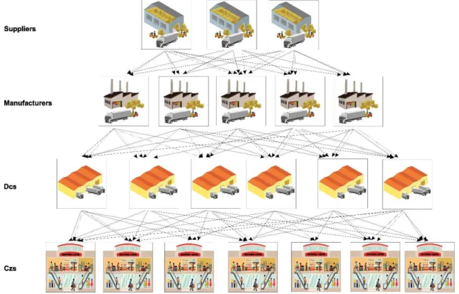
In this section, optimization of the network model objectives of an SC will be discussed, and then a mathematical model will be developed. While designing an SC network, the managers should make decisions on location and allocation of capacity to each of the facilities that is interrelated with others. In the developed model, a public SC network with four different levels is considered. The first level is the customer zone (CZ) that will be actually the place for selling the products to customers. The second level includes the distribution centers (DC), which will be indeed the place for transferring the products to customers. The third level is, in fact, the factory or the manufacturing sector. And in the fourth section, the suppliers are located. The income resulted from selling the products will be spent for the equipment, human force, transportation, purchasing the required material, and inventory. In order to reduce the complexity of the mathematical modeling and force the model to converge to optimal solution, a minimum demand is assumed for the given product, so that in all the scenarios, such minimum demand should be met. Figure 1 demonstrates the structure of the studied chain.
Figure 1. Structure of the studied chain
3-1- Hypotheses
Manufacturing the product requires three raw materials.
Capacity of the suppliers for raw materials varies, and the costs of production and transportation of each unit of raw material in each of the suppliers is specified.
Production and maintenance costs for each product and distribution costs for each factory and distribution center are constant.
Inventory cost for each product and cost of transferring the product from each distribution center to each of the customer zones are constant.
Minimum finishing rate should be maintained.
3-2- Model inputs
Number of suppliers and their capacity for each raw material
Number of potential zones of factories and distribution centers as well as their capacity
Cost of creating each raw material in each of the suppliers as well as the cost of transferring from each supplier to each factory
Costs of production and inventory in each factory
Cost of transporting each unit of product from the factory to each distribution center
Cost of efficiency of the product in each of these distribution centers and cost of transporting each product from that center to the customer zone
Number of customer zones and their demands
Minimum finishing rate (a percentage of the met demand) that should be maintained.
3-3- Model outputs
Amount of each raw material that should be transported from a supplier to a factory. Number of factories and their location
Flow of materials from the intended factory to distribution centers Number of distribution centers and their location
Allocation of customer zones to distribution centers
3-4- Objective functions
Minimizing the total SC cost, which includes raw material production, transportation, location of factories, production and maintenance, distribution of the products from factories to distribution centers, efficiency cost of the distribution centers, and cost of transporting from the distribution centers to the customer zone
Maximizing the finishing rate
The production ability indicates the company’s ability to meet the customer’s order with regard to the available inventory. The inventory shortage occurs when the manufacturer receives the customer’s order but lacks sufficient inventory. The product’s finishing rate (FR) and cycle service level (CSL) are criteria for measuring the product’s availability. The product’s finishing rate is a fraction of the product demand, which is met through production and maintenance; however, the cycle service level is a fraction of the cycle replacement, which is finished by meeting the demands of all the customers. In the following sections, the decision parameters and variables in a problem will be presented.
3-5- Notations
Indices:
j customer areas and demand zones
e warehouses
i potential zones of location of factories
h suppliers
Parameters:
Dj Demand of the customer j
ki Potential capacity of the factory i
ke Potential capacity of the warehouse e
sch Supply capacity in the supplier h for the component c
fi Annual fixed cost to setup the factory i
fe Annual fixed cost to setup the warehouse e
cchi Cost of preparing and transporting the component c from the supplier h to the factory i
cie Cost of manufacturing and transporting from the factory i to the warehouse e
cej Cost of transporting from the warehouse e to the customer j zone
ICi holdingcost in the factory i
IEe holding cost in warehouse e
Decision variables:
yi 1if the i is constructed, otherwise 0
ye 1if the warehouse e is constructed, otherwise 0
xhci Amount of the component c transported from the supplier h to the factory i
xie Amount of the final product transported from the factory i to the warehouse e
xej Amount of the final product transported from the warehouse e to the customer j
3-6- Mathematical model
1
1 1 1 1 1 1 1 1 1
. . ( ). ( ). .
p
n t n l n t t m
i i e e chi i chi ie i ie ej ej
i e i h e i e e j
Min z f y f y c IC x c IE x c x
= = = = = = = = =
=
∑
+∑
+∑∑∑
+ +∑∑
+ +∑∑
(1)1 1 2
1
t m ej e j
m j j
x Max z
D
= =
=
=
∑∑
∑
(2). .
s t
. ,
n
hci ch h i
x ≤S y ∀h c
∑
(3)1
t
ej j e
x D j
=
≤ ∀
∑
(4)1
. t
ie i i e
x K y i
=
≤ ∀
∑
(5)1
. m
ej e e j
x K y e
=
≤ ∀
∑
(6)1 1
0 ,
l t
hci ie
h e
x x i c
= =
− ≥ ∀
1
0
n m
ie ej
i j
x x e
=
− ≥ ∀
∑
∑
(8)1 1
0.8 1
t n ej e j
j j
x D
= =
≤ ≤
∑∑
∑
(9), , {0,1} , ,
i e h
y y y ∈ ∀i e h (10)
, , 0 , , , ,
ie ej hci
x x x ≥ ∀i e j h c (11)
The objective function (1) demonstrates minimization of the total cost of implementing and operationalizing of network (including fixed and variable costs), and the objective function (2) represents maximization of the finishing rate.
Constraint (3) indicates that the total amount of the products sent from the supplier cannot be greater than the supplier’s capacity. Constraint (4) implies that the demand should be met at any point in the market. Constraint (5) states that no factory can supply commodities more than its capacity; similarly, for the constraint (6), the supplier serves in the same way. Constraint (7) expresses that the amount sent from the factory should not be greater than the flow of the raw material entering the factory. Constraint (8) suggests that the amount sent from the warehouse should not exceed the amount entering the warehouse. Constraint (9) states that the level of meeting a demand, regarding the finishing rate, should be in the range of 80-100%. Finally, the constraints (10) and (11) determine the type of decision variables.
4- Solution approach
4.1. Multi-objective optimization concepts
General multi-objective optimization can be considered as a continuous process of optimizing two or more conflicting objectives with regard to certain constraints. Since the multi-objective optimization has multiple objective functions, the solution method seeks to find exchanges between the obtained solutions. The concept of Pareto optimality in the multi-objective optimization was introduced by Pareto in 1986 as follows:
Where the point x*∈Ωwill be the Pareto optimal solution if ( (fi x*)≤fi( ))x ∀ ∈i I x, ∈ Ω, where
{
1, 2,....,
}
I
=
K
and there is at least onei
∈
I
so that ( (fi x*)pfi( ))x ∀ ∈i I .This definition states that X* is the Pareto optimal solution if there is no reasonable solution that can
reduce some of the measures without simultaneous increase in at least one of the objectives. The multi-objective optimization algorithm uses the concept of dominance to obtain the optimal solution. In this algorithm, two solutions are compared with each other, so that it is evaluated whether one dominates the other one or not. If there are M objective functions, then the solution X will dominate the solution Y in case that both of the following conditions are true:
1. The solution X is worse than Y in none of the objectives.
2. The solution X is better than Y in at least one of the M objectives.
If only one of the above conditions is true, then the solution X will not dominate the solution Y. In the multi-objective optimization, since we face more than one objective for optimization, there is not only a single optimal solution that optimizes all the objectives. The output results include a set of optimal solutions that have different values in different functions. This set of solutions is called non-dominant set. The following two conditions should be true for each member of the non-dominant set:
1. Both non-dominance sets should be non-dominant relative to all of each other’s members.
2. Any solution that doesn’t belong to the non-dominant set is dominated by one of the members of
the non-dominant set. Such non-dominant set is known as the set of Pareto optimal solutions. Due to minimization of the total SC costs and maximization of the finishing rate and, as a result, the conflict of these two objectives in terms of their nature, it would be impossible to obtain an optimal solution for this problem; therefore, in such a case, it is attempted to obtain optimal solutions that determine appropriate policies for the chain. Thus, the set of Pareto solutions and its decision variables are designed such that the decision maker can select the Pareto solutions to meet his need.
4-2- Introduction of particle swarm algorithm
Particle swarm algorithm (PSO) is one of the newest population-centered techniques for optimization of the models (Kennedy and Eberhart, 1995). In this algorithm, some of the solutions are considered as the particles moving in the solution’s space. PSO acts based on the behavior of the societies that are interrelated both socially and individually (such as the birds looking for food) (Coello, 1999). A bird might find its food whether through group cooperation with other birds or lonely.
In the PSO algorithm, each individual (particle) indicates a solution in the N-dimensional space; besides, each particle is informed of the best experience of his own and others. Each particle changes its path with regard to the equations (12) and (13) (Coello et al. 2002).
1 1 2 2
* * * ( ) * * ( )
ij ij ij ij gi ij
v =w v +c r p −x +c r p −x (12)
ij ij ij
x =x +v (13)
In equations (12) and (13), w is a constant factor that is affected by the local and general ability of the algorithm, vij is the speed of the i
th
particle in the jth dimension, c1 and c2 are the weights that are affected
by the personal and social movements, r1 andr2 are the random numbers from uniform distribution
between 1 and 0, pij represents the best value found by the i
th
particle, and pgi indicates the best solution found by all the particles. Once the particle’s speed is updated, the new position of the ith particle is
calculated in the jth direction. Eventually, all the particles resemble a huge flock of birds that, in order to
find their food, are moving toward the regions with more foods; in fact, they are approaching an optimal solution with more fitness function. The PSO algorithm is highly regarded due to its simplicity of implementation and capability of rapid convergence to the reasonable solution. In this algorithm, better searching and finding the optimal solution requires adjusting a few parameters.
Operators of the MOHPSO algorithm should be selected properly. In this algorithm, the speed should be converted into the probabilistic mode, which is the chance of getting a value of 1 for the particle. Here,
the particle’s speed was calculated using equations (14), (15), and (16), where c1 and c2 are constant and
equal numbers, pBestlis the best solution of any particle 1, nBesttis the best total solution (leader), w
is the constant inertia value and equal to 0.5, r1 and r2 are random numbers, Vit is the particle’s speed,
it
x is particle position, Vmaxis equal to 4, andsplis the probability between 0 and 1. Then, the random
number
ρ
is produced in [0, 1], and the particle’s new position is determined using equation (17) (Che,2012).
(
)
(
)
, 1 1 1 , 2 2 ,
. . . .
it l t l l t t l t
V =w V − +c r pBest −x +c r nBest −x (14)
max l t, max
V V V
− ≤ ≤ (15)
,
1
1 1 Vl t
sp
e−
=
+ (16)
1 ,
1 0 l t
sp x
Otherwise
ρ
≤
=
In this algorithm, the random mutation with rate of 0.2 was used. In general, the MOHPSO algorithm’s steps can be expressed as follows:
Step-one: Generating the initial solutions randomly
Step-two: Calculating the fitness value for each of the initial solutions based on the defined objective functions
Step-three: Determining the non-dominant solutions generated in the set of initial solutions
Step-four: Determining the leader solution from among the available solutions to create neighborhood in the solutions
Step-five: Creating new solutions based on equations (14) and (15)
Step-six: Updating the best personal experience of each particle. If the particle’s new position dominates the best experience, then the new position will replace best experience, and if none of them dominate the other one, one of the above positions will be randomly considered as the best experience.
Step-seven: Adding the non-dominated members of the current population to the external memory Step-eight: Eliminating the non-dominated members of the external memory
Step-nine: Eliminating the members exceeding the external memory’s capacity
The probability of elimination of the members exceeding the external memory’s capacity is obtained through Equation (18). In this equation, ii is the cell number. After determining the probabilities of elimination of the additional solutions by Roulette Wheel method, the additional solutions are removed.
_ , 0 _ 1, 1
ii
ii
n
i ii ii
n i
j
e
del prob del prob iq
je
= ≤ ≤
∑
=∑
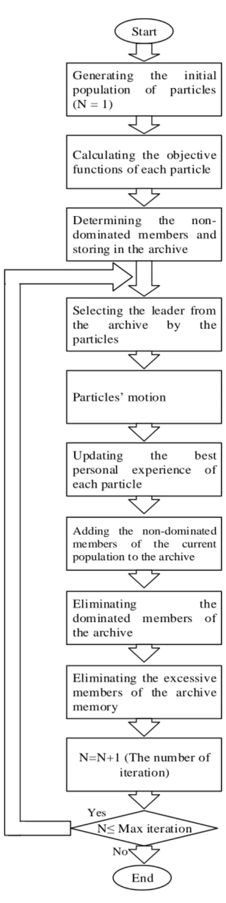
(18)Step-ten: Stop in case of fulfillment of the finishing condition, otherwise going to the third step. In figure 2, the MOHPSO algorithm’s steps are represented as flowchart.
Yes
No
Start
Generating the initial population of particles (N = 1)
Calculating the objective functions of each particle
Determining the non-dominated members and storing in the archive
Selecting the leader from the archive by the particles
Particles’ motion
Updating the best personal experience of each particle
Adding the non-dominated members of the current population to the archive
Eliminating the dominated members of the archive
Eliminating the excessive members of the archive memory
N=N+1 (The number of iteration)
N≤ Max iteration
End
4-3-Two-objective genetic algorithm (NSGA II)
Genetic algorithm is one of the heuristic algorithms for solving the problems, which has been derived from biological modeling of the animals’ population. In this algorithm, characteristics of the animals’ generation is resembled to the value of the objective functions and improvement of the generations’ characteristics over time, and emersion of the new generations from intercourse of the previous generations is analogized to the improvement of the value of the objective function; in other words, this algorithm uses the Darwin's natural selection principle to find a formula or the optimal solution in order to predict or compare the pattern. The NSGA II general algorithm, as one of the multi-objective genetic modes, is as follows:
1. Creating the initial population
2. Calculating the fitting criteria
3. Sorting the population based on the dominance conditions
4. Calculating the swarm distance
5. Selection; as soon as the initial population is sorted based on the dominance conditions, the
swarm distance will be calculated, and selection from among the initial population will begin. This selection is carried out based on two elements:
• Population ranking: populations are selected at lower ranks
• Distance calculation: Assuming that p and q are two members of a same rank, the member
with higher swarm distance will be selected. It should be noted that the selection priority is primarily based on the ranking and then on the swarm distance.
6. Generating new children through crossover and mutation, and integration of the initial population
with the population obtained from crossover and mutation
7. Replacing the parent population with the best members of the population integrated in the
previous steps
In the first step, members with lower ranks are replaced for the previous parents, and then are sorted based on the swarm distance. The initial population and the population resulted from crossover and mutations are sorted primarily based on ranking, and then those with lower ranks are eliminated. In the next step, the remaining population is sorted based on the swarm distance (Coello et al. 2007).
5- Numerical results and analysis
5-1-Results of generated numerical examples and comparing two algorithms
In order to evaluate performance of the proposed algorithm, the MOHPSO algorithm’s performance should be assessed on the examples. According to the multi-objective structure of the mathematical model as well as the proposed algorithm, the comparison is carried out by one of the most powerful multi-objective optimization algorithms, namely the NSGA II algorithm. So the structure of the two algorithms was encoded in MATLAB R2014 software.
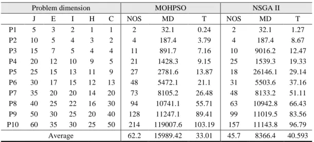
Hence, 10 examples were designed with different dimensions, and solved by MOHPSO and NSGA II algorithms. Since there is no accurate benchmark for the investigated problem, the sample examples were randomly generated from a uniform distribution. In table 2, dimensions of the examples are specified, and also the results of implementation the two given algorithms are compared.
Table 2. Dimensions of examples and Problem dimension I E J 2 3 5 P1 4 5 10 P2 5 7 15 P3 10 12 20 P4 11 13 15 25 P5 12 15 17 30 P6 14 20 20 35 P7 16 22 25 40 P8 20 25 30 50 P9 25 30 35 60 P10 Average
In table 2, dimensions of the problem show the number of customers, number of warehouses, number of factories, number of suppliers, and
compared using MD and NOS indices of the meta-heuristic algorithm, through Equation (19):
max min 2 max min 2
1 1 2 2
( ) ( )
MD = Z −Z + Z −Z
Also, T is the time of algorithm implementation and MD, the higher the efficiency of the
According to table 2, comparing revealed that the MPHOSP algorithm and
Pareto frontier, respectively. Thus, the MOHPSO algorithm detailed investigation showed that
problem, and in other cases, the MOHPSO had been better. In Figure index for both algorithms in different examples.
Figure 3. Comparing NOS index in two MOHPSO and NSGA II algorithms
examples and comparing the efficiency of MOHPSO and NSGA II MOHPSO Problem dimension NOS T MD NOS C H 2 0.24 32.1 2 1 1 4 3.79 187.4 4 2 3 10 7.16 891.7 11 4 4 25 9.15 1428.3 21 5 9 18 13.87 2781.6 27 9 11 31 21.1 5472.1 48 13 12 48 26.48 8105.2 73 20 14 63 55.71 10741.1 94 30 16 99 89.41 11247.1 128 40 20 157 103.19 119007.6 214 50 25 45.7 33.01 15989.42 62.2
able 2, dimensions of the problem show the number of customers, number of warehouses, number of factories, number of suppliers, and number of components, respectively. The studied algorithms were
MD and NOS indices. The NOS states the number of Pareto solutions in the final , and MD expresses the maximum expansion. This
max min 2 max min 2
1 1 2 2
( ) ( )
MD = Z −Z + Z −Z
time of algorithm implementation in seconds. Clearly, the higher higher the efficiency of the algorithm in finding the Pareto frontier.
2, comparing the MOHPSO and NSGA II algorithms based on the
MPHOSP algorithm and NSGA II algorithm found nearly 62 and 45 solutions at the Thus, the MOHPSO algorithm had the superiority in this index.
that the NSGA II algorithm has had better NOS index problem, and in other cases, the MOHPSO had been better. In Figure 3 presents index for both algorithms in different examples.
Comparing NOS index in two MOHPSO and NSGA II algorithms
MOHPSO and NSGA II algorithms NSGA II T MD 1.27 32.1 8.67 187.4 12.47 9016.2 19.33 1539.3 29.14 26146.1 37.16 5503.6 51.11 8133.2 66.43 10942.8 83.56 11019.5 96.79 11143.8 40.593 8366.4
able 2, dimensions of the problem show the number of customers, number of warehouses, number The studied algorithms were Pareto solutions in the final output This index is calculated
(19)
Clearly, the higher is the value of NOS Pareto frontier.
based on the NOS index NSGA II algorithm found nearly 62 and 45 solutions at the had the superiority in this index. A more better NOS index merely in the P4 presents the values of the NOS
Also, according to table 2, the MD i MOHPSO algorithm had better MD value units between the two algorithms in algorithm has had the superiority as well
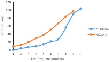
However, besides the solution
algorithm, which must be analyzed and assessed. Figure 4 algorithms.
Figure
As shown in figure 4, also in terms of
relative superiority to the NSGA II algorithm and provided the solutions in the shortest possib Therefore, according to the comparisons, efficiency of
the solution quality and speed; therefore algorithm.
5-2- Case study results
To show capability of the proposed algorithm, a real case study is considered on mountain bikes from a four-level supply chain with a
distribution centers, and 7 customer zones.
suppliers to the relevant factories. In factories, these components are assembled and the final bicycle is ready to be transferred to the warehouse and then
company is seeks to locate the 5
it can meet the 30-unit demand of 7 areas using 6 warehouses with a total capacity of 82 units. level of the SC network, the suppliers provi
product. The capacity of suppliers, factories, warehouses, shown in table 3. The production costs of a component manufacturing plants are shown in the
and transportation costs of each
maintenance and transportation costs as well as th the chain are shown in table 6.
Information such as the components of the product, consumption, and supply chain capacity has been determined through interviews with relevant experts of the
costs are determined with respect to position of each of the supply chain components and also the distance between them.
This problem and the final results
able 2, the MD index is the same as NOS. In 8 cases out of the MOHPSO algorithm had better MD value; however, in general, there is an average
two algorithms in terms of the average of this index. Thus, in this index, t the superiority as well.
solution quality, the solution time is another dimension of be analyzed and assessed. Figure 4 represents the solution
Figure 4. Solution time in MOHPSO and NSGA II algorithms
in terms of the solution time, the MOHPSO algorithm NSGA II algorithm and provided the solutions in the shortest possib
comparisons, efficiency of the MOHPSO algorithm is
speed; therefore, in the following section, a real case study is implemented
proposed algorithm, a real case study is considered on level supply chain with a network structure with 3 suppliers, 5 distribution centers, and 7 customer zones. The primary components are sent by the
suppliers to the relevant factories. In factories, these components are assembled and the final bicycle is ready to be transferred to the warehouse and then delivered to the customers. In this problem, the 5 manufacturing plants with a total capacity of 142 units per month, so that demand of 7 areas using 6 warehouses with a total capacity of 82 units.
network, the suppliers provide all the three types of raw material for manufacturing a The capacity of suppliers, factories, warehouses, as well as the fixed costs for each
3. The production costs of a component and transportation costs shown in the table 4. The production variable inventory
costs of each demanded shipment to each customer are shown in tion costs as well as the manufacturing costs for each unit
Information such as the components of the product, consumption, and supply chain capacity has been determined through interviews with relevant experts of the bicycle production company
determined with respect to position of each of the supply chain components and also the distance
results were analyzed by considering two conflicting objectives.
out of the 10 examples, the , in general, there is an average difference of 7600 Thus, in this index, the MOHPSO
time is another dimension of the meta-heuristic represents the solution time in the two
time in MOHPSO and NSGA II algorithms
MOHPSO algorithm could have the NSGA II algorithm and provided the solutions in the shortest possible time.
MOHPSO algorithm is proved in terms of real case study is implemented by this
proposed algorithm, a real case study is considered on supplying the network structure with 3 suppliers, 5 factories, 6 ponents are sent by the domestic and foreign suppliers to the relevant factories. In factories, these components are assembled and the final bicycle is the customers. In this problem, the plants with a total capacity of 142 units per month, so that demand of 7 areas using 6 warehouses with a total capacity of 82 units. At the first three types of raw material for manufacturing a fixed costs for each factory are costs of each unit to the inventory, manufacturing costs, are shown in table 5. The e manufacturing costs for each unit at the third level of
Information such as the components of the product, consumption, and supply chain capacity has been production company. The transport determined with respect to position of each of the supply chain components and also the distance
Table 3. Capacity of suppliers, capacity of factories, fixed costs for each factory, and capacity of warehouses Capacity Warehouse Fixed cost Capacity Factory Element Supplier capacity c3 c2 c1 15 wh1 7650 18 p1 50 62 36 1 12 wh2 3500 24 p2 55 65 40 2 14 wh3 500 37 p3 60 70 42 3 13 wh4 4100 22 p4 12 wh5 2200 41 p5 16 wh6
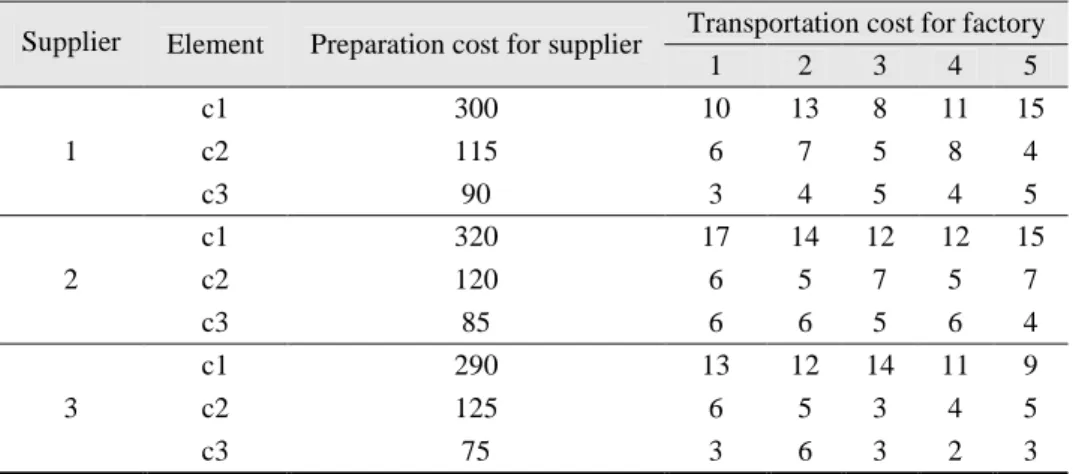
Table 4. Production costs of a component and transportation cost of each unit to the manufacturing plants
Transportation cost for factory Preparation cost for supplier
Element Supplier 5 4 3 2 1 15 11 8 13 10 300 c1
1 c2 115 6 7 5 8 4
5 4 5 4 3 90 c3 15 12 12 14 17 320 c1
2 c2 120 6 5 7 5 7
4 6 5 6 6 85 c3 9 11 14 12 13 290 c1
3 c2 125 6 5 3 4 5
3 2 3 6 3 75 c3
Table 5. Production variable inventory as well as the manufacturing and transportation costs of each shipment
unit to each of the customer zones
Inventory cost Production cost Warehouse Factory wh6 wh5 wh4 wh3 wh2 wh1 50 3900 20 18 17 18 12 7 1 45 2010 17 15 13 11 10 12 2 55 1945 21 18 15 14 10 8 3 48 1855 18 13 14 13 12 10 4 52 1975 12 11 15 11 10 8 5
Table 6. Holding and transportation costs as well as the manufacturing costs for each unit at the third level of the
chain Holding cost Customer Warehouse 7 6 5 4 3 2 1 55 4 3 7 6 9 3 8 wh1 50 8 2 3 6 7 8 5 wh2 60 4 5 7 6 8 3 9 wh3 54 8 4 5 2 2 9 3 wh4 55 4 9 4 9 3 6 7 wh5 45 9 2 3 8 7 6 5 wh6 3 5 4 6 4 5 3 Monthly demand
For this problem, minimizing the total costs and maximizing the finishing rate are carried out by considering that the minimum finishing rate should be 80% of the real demand. On the whole, there are 128 decision variables and 48 constraints. Solution of this problem solution is to obtain 7 Pareto optimal solutions. The final decision is that ranking is performed out of these solutions based on some certain criteria. This ranking is one of the most important decision problems for the decision maker. This decision might also be changed every year with regard to the demand and costs variations.
In table 7, the Pareto solutions of the particle swarm algorithm are specified. Each of the non-dominant solutions is in the form of a scenario for implementation and execution. Table 8 shows the optimal flow of the material from the suppliers to the factory with regard to Pareto.
Table 7: Resulted Pareto
Real demand The satisfied
demand level Supply chain
cost Non-Dominated
solution (scenario)
30 30
159306 1
30 29
149385 2
30 28
140629 3
30 27
129904 4
30 26
117818 5
30 25
107290 6
30 24
100480 7
Table 8: Optimized flow of the materials in 7 scenarios Element 1 Element 1 Element 1 Factory 3 2 1 3 2 1 3 2 1 Scenario 1 0 12 0 0 0 10 8 0 0 1 0 22 0 0 12 10 11 0 5 2 0 12 0 0 0 18 0 0 15 3 0 0 15 0 12 0 0 0 11 4 0 0 0 0 0 0 0 0 0 5 Scenario 2 0 0 0 8 0 0 4 1 0 1 0 0 12 9 0 0 0 18 0 2 20 20 0 0 0 17 0 9 10 3 0 0 0 0 0 0 0 0 0 4 0 0 9 0 0 10 0 11 0 5 Scenario 3 14 14 0 5 0 5 10 0 7 1 9 9 0 0 0 8 6 0 0 2 0 0 0 0 0 0 0 0 0 3 0 0 0 7 0 0 0 0 8 4 0 0 0 0 0 0 0 0 0 5 Scenario 4 0 0 0 0 0 0 0 0 0 1 0 0 0 0 0 0 0 0 0 2 0 0 0 21 0 0 0 0 23 3 18 18 0 0 0 16 15 0 0 4 22 22 0 0 0 0 17 0 0 5 Scenario 5 0 0 3 8 12 0 0 11 0 1 7 7 0 0 0 6 0 6 0 2 0 0 0 0 0 0 0 0 0 3 0 0 0 12 2 0 0 0 10 4 0 0 0 0 0 0 0 0 0 5 Scenario 6 0 0 0 0 0 0 0 0 0 1 0 0 0 19 14 0 11 7 0 2 0 0 0 12 0 0 0 5 6 3 0 0 0 0 0 0 0 0 0 4 0 0 7 0 0 12 9 0 0 5 Scenario 7 11 11 0 0 10 0 9 0 0 1 0 0 0 0 0 0 0 0 0 2 0 0 20 0 0 0 0 0 17 3 0 0 0 0 0 0 0 0 0 4 0 0 0 0 0 0 0 0 0 5
Subsequently, for a more detailed investigation of the results of the case study, first, the Pareto chart of solutions derived from the case study should be presented. In Figure 5, the Pareto chart of the case study is presented.
Figure 5.
As seen in figure 5, in case of looking for is reduced as well; thus, the conflicts of the obj On the other hand, with respect to
given meta-heuristic algorithm. Pareto solutions will be evidently
Also, since several optimal solutions have been found for this problem, the have the opportunity to evaluate different scenarios in
of the problem, which cannot be presented in the structure of the most appropriate one.
6- Conclusion
In this research, a mathematical model was developed for location and allocation of the facilities in a four-level supply chain. In this model, capacity of
production and maintenance costs transportation costs were considered
simultaneous optimization of the costs and customer satisfaction in the hierarchical location of well as the use of multi-objective evolutionary meta
presented in this research, which
in order to find the Pareto optimal solutions, The obtained solutions showed tha
provided. The comparisons between this algorithm and NSGA II algorithm efficiency of the proposed algorithm in solving the problems related to the hierarchi supply chain (also see figure 3 and
heuristic MOHPSO algorithm showed the customer satisfaction (see f suggested to consider the reliability
. Pareto chart of the solutions obtained from the case study
5, in case of looking for the scenarios with lower cost, the customer
, the conflicts of the objectives presented in this research can be shown properly. On the other hand, with respect to the 80% meeting of the demand, only 7 scenarios are
heuristic algorithm. If this constraint is reduced to lower than 80%, the number of evidently larger.
optimal solutions have been found for this problem, the opportunity to evaluate different scenarios in terms of executability as well as
cannot be presented in the structure of the mathematical models
, a mathematical model was developed for location and allocation of the facilities in a level supply chain. In this model, capacity of the factories and distribution centers
production and maintenance costs had certain and constant values; furthermore
considered besides this location. The basic innovation of this research simultaneous optimization of the costs and customer satisfaction in the hierarchical location of
objective evolutionary meta-heuristic algorithms for optimization.
, which was based on the particle swarm algorithm, was developed for the model Pareto optimal solutions, ultimately leading to a number of
solutions showed that by trade-off between the objectives, different optimal solutions can be . The comparisons between this algorithm and NSGA II algorithm in
proposed algorithm in solving the problems related to the hierarchi
igure 3 and figure 4). At the end, the case study of mountain bike using showed that the set of Pareto solutions were executable and could achieve
figure 5 and table 7). As further research on the proposed model, it is reliability inventory and risk factor for the chain as well as the reliability costs.
case study
scenarios with lower cost, the customer satisfaction level in this research can be shown properly. 7 scenarios are presented by the this constraint is reduced to lower than 80%, the number of the found
optimal solutions have been found for this problem, the SC management would as well as the hidden aspects mathematical models, and finally choose
, a mathematical model was developed for location and allocation of the facilities in a factories and distribution centers, as well as the ; furthermore, the inventory and innovation of this research was in the simultaneous optimization of the costs and customer satisfaction in the hierarchical location of the SC as heuristic algorithms for optimization. The algorithm was developed for the model a number of non-dominant solutions. objectives, different optimal solutions can be in table 2 indicated high proposed algorithm in solving the problems related to the hierarchical location in the of mountain bike using meta-were executable and could achieve
the proposed model, it is inventory and risk factor for the chain as well as the reliability costs.
References
Che, Z. H. (2012). A particle swarm optimization algorithm for solving unbalanced supply chain planning problems. Applied Soft Computing Journal, 1279–1287.
Coello, C. a. C. (1999). A Comprehensive Survey of Evolutionary-Based Multiobjective Optimization Techniques. Knowledge and Information Systems, 1(3), 269–308.
Coello Coello, C. A., Lamont, G. B. and Veldhuizen, D. a Van (2007). Evolutionary Algorithms for Solving Multi-Objective Problems (Vol. 5). New York: Springer.
Coello Coello, C. A. and Lechuga, M. S. (2002). MOPSO: A proposal for multiple objective particle swarm optimization. Proceedings of the 2002 Congress on Evolutionary Computation, CEC 2002, 1051– 1056.
Erlenkotter, D. (1981). A comparative study of approaches to dynamic location problems. European
Journal of Operational Research, 6(2), 133–143.
Haji abbas, M. and Hosseininezhad, S. J. (2016). A robust approach to multi period covering location-allocation problem in pharmaceutical supply chain. Journal of Industrial and Systems Engineering, 9(special issue on location allocation and hub modeling), 71–84.
Hakimi, S. L. (1964). Optimum Locations of Switching Centers and the Absolute Centers and Medians of a Graph. Operations Research. INFORMS, 12(3), 450–459.
Jena, S. D., Cordeau, J. F. and Gendron, B. (2016). Solving a dynamic facility location problem with partial closing and reopening. Computers and Operations Research, 67, 143–154.
Kennedy, J. and Eberhart, R. (1995). Particle swarm optimization. Neural Networks, 1995. Proceedings.,
IEEE International Conference on, 4, 1942–1948.
Latha Shankar, B., Basavarajappa, S., Chen, J. C. H. and Kadadevaramath, R. S. (2013). Location and allocation decisions for multi-echelon supply chain network - A multi-objective evolutionary approach.
Expert Systems with Applications, 40(2), 551–562.
Li, T., Song, R., He, S., Bi, M., Yin, W. and Zhang, Y. (2017). Multiperiod Hierarchical Location Problem of Transit Hub in Urban Agglomeration Area. Mathematical Problems in Engineering. Hindawi Publishing Corporation, 2017.
Marianov, V. and Serra, D. (2001). Hierarchical location-allocation models for congested systems.
European Journal of Operational Research, 135(1), 195–208.
Mirchandani, P. B. and Francis, R. L. (1990). Discrete Location Theory.
Montoya, A., Vélez–Gallego, M. C. and Villegas, J. G. (2016). Multi-product capacitated facility location problem with general production and building costs. NETNOMICS: Economic Research and Electronic
Networking, 17(1), 47–70.
Mostaghim, S. and Teich, J. (2004). Covering Pareto-optimal fronts by subswarms in multi-objective particle swarm optimization. Proceedings of the 2004 Congress on Evolutionary Computation (IEEE Cat.
No.04TH8753), 2, 1404–1411.
Nguyen, V.-P., Prins, C. and Prodhon, C. (2012). A multi-start iterated local search with tabu list and path relinking for the two-echelon location-routing problem. Engineering Applications of Artificial
Intelligence, 25(1), 56–71.
problems. 2002 ACM Symposium on Applied Computing (SAC 2002), 603–607.
ReVelle, C. S., Eiselt, H. A. and Daskin, M. S. (2008). A bibliography for some fundamental problem categories in discrete location science. European Journal of Operational Research, 184(3), 817–848. Scott, A. J. (1971). Dynamic Location-Allocation Systems: Some Basic Planning Strategies. Environment
and Planning A. SAGE Publications, 3(1), 73–82.
Shahabi, M., Akbarinasaji, S., Unnikrishnan, A. and James, R. (2013). Integrated Inventory Control and Facility Location Decisions in a Multi-Echelon Supply Chain Network with Hubs. Networks and Spatial
Economics, 13(4), 497–514.
Tsou, C. S., Yang, D. Y., Chen, J. H. and Lee, Y. H. (2011). Estimating exchange curve for inventory management through evolutionary multi-objective optimization. African Journal of Business
Management, 5(12), 4847–4852.
Wang, X. and Ouyang, Y. (2015). A continuum approximation approach to competitive facility location design under facility disruption risks. Transportation Research Part B: Methodological, 50, 90–103. Warszawski, A. (1973). Multi-Dimensional Location Problems. Journal of the Operational Research
Society, 24(2), 165–179.
Weber, A. (1909). Theory of industrial location.
Yasenovskiy, V. and Hodgson, J. (2007). Hierarchical location-allocation with spatial choice interaction modeling. Annals of the Association of American Geographers, 97(3), 496–511.
Yu, V. F., Normasari, N. M. E. and Luong, H. T. (2015). Integrated location-production-distribution planning in a multiproducts supply chain network design model. Mathematical Problems in Engineering, 2015.