A Universal Damping Function for Empirical Dispersion Correction on Density Functional Theory

A Universal Damping Function for Empirical Dispersion Correction

on Density Functional Theory

Yi Liu

_{and William A. Goddard III}

Materials and Process Simulation Center (M/C 139-74), California Institute of Technology, 1200 East California Blvd., Pasadena, California, USA 91125

A damped London dispersion interaction is generally adopted in empirical dispersion corrections on density functional theory (DFT), where dispersion parameters are determined empirically to reproduce correct dispersive interactions after assuming a damping function. The key to a successful dispersion correction is choosing an appropriate damping function. In this work we propose a single universal damping function that can represent several damping functions used in literatures with a few adjustable parameters. This universal damping function provides a unified formula that allows convenient comparison and flexible optimization in dispersion corrected DFT methods. Using the optimized universal damping functions and dispersion parameters, we develop dispersion correction methods for HF, B3LYP and PBE theories. We calculate the dispersive energies accurately for rare gas diatomic molecules and benzene dimers with an averaged error<4:1%.

[doi:10.2320/matertrans.MF200911]

(Received March 16, 2009; Accepted March 24, 2009; Published June 25, 2009)

Keywords: empirical dispersion correction, density functional theory, London dispersion, damping function

1. Introduction

Density functional theory (DFT)1,2) _{becomes a popular} quantum mechanics (QM) method in computational chem-istry because of the reduced computational cost compared with ab initio post Hartree-Fock (HF) quantum chemistry methods. Despite the great success of DFT in a wide range of applications, DFT failed to describe dispersive interactions in several cases as summarized below.

Pulay et al.3) _{employed GGA (BLYP) calculations on} rare gas dimers (He2, Ne2, Ar2), showing that BLYP yielded a purely repulsive interaction. Beckeet al.4)_carried out LDA (PW), GGA (LDA+BP), GGA/exactX (B3LYP), and GGA (Bhalf-and-half) calculations on six rare gas dimers (He2, Ne2, Ar2, HeNe, HeAr, and NeAr). They showed that LDA severely overestimated dissociation energies, whereas GGA (LDA+BP) and GGA (B3LYP) yielded repulsive potential curves. Becke’s half-and-half functional (BH&H) accidentally led to weak bindings, but it still severely underestimated the dissociation energies. It was recently found5) that BH&H qualitatively reproduced geometric and energetic details of parallel -stacked aromatic complexes. However, this is presumably due to fortuitous error cancellation. Hobza et al.6) _{applied BLYP,} B3LYP, and B3P86 DFT methods to study H-bonded, ionic, electrostatic and London clusters. All these methods failed completely to describe London-type clusters, for which no minimum was found on the potential energy surfaces (PES). Jeonget al.7)_{carried out SVWN, BLYP and} B3LYP studies on Cl2 (van der Vaals complex) and X-HCl (H-bonded complex) with large basis set [6-311++G (3df, 2pd)], and found that BLYP and B3LYP yielded much smaller binding energies than MP2 values. Sprik et al.8) used LDA, LDA+B, LDA+B+LYP methods to study intermolecular interaction of benzene dimer. Consistent

with previous studies of rare gas dimers, LDA exhibited a minimum on PES. However, this is fortuitous because the dispersive energy is not included in LDA. On the other hand, LDA+B and LDA+B+LYP yielded purely repulsive potentials.

The above brief review is not meant to be exhausted but should be convincing enough to prove the failure of DFT methods in those weakly interacting systems. The lack of dispersive interaction in DFT is a consequence of locality nature of the approximated exchange-correlation (xc) func-tionals adopted in DFT. It is inevitable to fix dispersion problems in DFT in order to study systems where the dispersive interaction plays an important role (e.g. biological molecules or molecular crystals). It has been shown that dispersive interactions can be incorporated into DFT quan-tum mechanically either through time-dependent DFT approaches9,10) _{or improved xc functionals.}11–18) _These improved first principle approaches are often more expensive than the conventional DFT methods, which limit their applications in large scale simulations and dynamics studies. On the other hand, empirical dispersion corrections provide a pragmatic way to account for dispersive interactions in DFT without losing computational efficiency.

The empirical dispersion correction methods are main focus of this work. The idea of empirical dispersion correction is to compute damped dispersive interactions empirically and add them into conventional DFT energies as correction terms. Various correction methods have been proposed, differing mainly in the choice of damping functions. Detailed comparisons among different correction methods can be found in Sec. 2. In this work, we propose a new damping function that can represent various damping functions by using a single formula with different choice of parameters. This unified damping function allows convenient comparison among existing correction methods at an equal rooting. More importantly, the universal damping function can be utilized as a flexible formula for further improve-ments on dispersion corrected DFT methods. In Sec. 3, we *_{Corresponding authors, E-mails: [email protected], [email protected].}

edu

demonstrate how the new universal damping function can be used to correct dispersions on DFT with examples of rare gas diatomic molecules and benzene dimers. Finally, we draw conclusions in Sec. 4.

2. Methods of Dispersion Correction on DFT

In the spirit of incorporating dispersive interaction into HF,19) _{most current empirical dispersion corrected DFT} (DFT-D) methods20–26) _{augment a damped London} disper-sion27)energy into conventional DFT:

EDFT-D¼EDFTþEdisp ð1Þ whereEDFT is a normal DFT energy, andEdisp a dispersion correction term. The dispersion correction can be expressed in terms of a damped multipole expansion:

Edisp¼

XN

ij;i<j Xm

k¼3

fdampðrijÞ C2k

r_ij2k !

¼ X

N

ij;i<j

fdampðrijÞ C6

r6 ij

þC8

r8 ij

þC10

r10 ij

þ. . . !

XN

ij;i<j

fdampðrijÞ C6

r6 ij

ð2Þ

where fdamp is a damping function. C6 etc. are dispersion

parameters for an atom type. TheC6 dispersion parameters

between unlike atoms are calculated based on a geometrical mean Cij¼ ðCiCjÞ1=2. N is the number of subsystems (e.g. atom or moleculei).rijis the distance betweeniand j. The first sum runs over all pairs of subsystems, while the second sum represents a series of multipole expansion, describing the asymptotic behavior of dispersion. Higher order terms beyond 1=r6 _{are neglected as an approximation in most}

current DFT-D methods.

Various DFT-D methods in literatures differ mainly in the choice of different damping functions. Wu and Yang20) proposed two damping functions:

fdampðrijÞ ¼ 1exp cdamp rij R0 ij

!3 2

4

3 5 8

< :

9 = ; 2

ð3Þ

wherecdamp¼3:54was used.R0ij is a sum of vdW radii of atom i and j. Hereafter the damping function, eq. (3), is denoted as WY1 function. The other damping function is

fdampðrijÞ ¼

1

1þexp rij

R0 ij

1 !

" # ð4Þ

where¼23:0. It was determined by requiringfdamp ¼0:99 atr¼1:2R0. Equation (4) is a Fermi function. Hereafter we

denote this specific damping function as WY2 function. Wu and Yang concluded that WY1 was better than WY2 in their work because WY1 decays more slowly than WY2. How-ever, Zimmerli et al.26) obtained an opposite conclusion: WY2 was better for correcting HCTH, B3LYP, PW91 and PBE methods in the study of water benzene clusters.

WY2 damping function was further modified by Grimme et al.21,22)_{and Jureckaet al.}23)_{by adding scaling factors.}

fdampðrijÞ ¼

s6

1þexp d rij

sRR0ij

1 !

" # ð5Þ

Equation (5) has four parameters, namely, s6ð1:0Þ, d

(23), sR (1:0) and R0ij. s6 is a global scaling parameter

introduced by Grimme et al. sR is a scaling parameter associated with xc functionals and the uncertainty of vdW radii.d reflects the steepness of exponents. To correct some specific functionals,s6anddneed to be tuned. The damping

function eq. (5) was used by Jureckaet al.23)WhensR¼1:0, eq. (5) recovers Grimme’s formula.21,22) When s6¼1:0,

d¼23, sR¼1:0, eq. (5) recovers WY2 function. Thus Grimme’s and Jurecka’s damping functions can be consid-ered as variants of WY2 function.

Elstner et al.24) used the following damping function to correct an extended tight-binding method for dispersion:

fdampðrijÞ ¼ 1exp d rij

R0_ij !N

" #

( )M

ð6Þ

whered¼3:0,N¼7,M¼4,R0

ij¼3:8A˚ for the first row elements, and R0

ij¼4:8A˚ for the second row elements. Hereafter the damping function, eq. (6), is denoted as EHFSK function. Zimmerliet al.26)_{found EHFSK function} was not as good as WY2 in their studies of water benzene clusters.

Ortmann et al.25) used an exponential decay potential as follows:

fdampðrijÞ ¼1exp rij R0 ij

!n

" #

ð7Þ

where ¼7:5104 _{and n¼8. These parameters were}

determined to reproduce the c-lattice constant of graphite. The damping function, eq. (7), is hereafter denoted as OBS function.

The literature review above shows that the damping functions currently used in the field vary substantially from function forms to parameters. The behaviors of chosen damping functions affect directly the quality of subsequent fitting of dispersion parameters. Thus it is critical to choose a good damping function in DFT-D methods. A damping function is normally designed with some constraints, e.g., it should approach to one at large distance but to zero at short distance. Despite these simple constraints, the choice of damping functions in literatures is somewhat arbitrary without rigorous justification and full optimization. Contro-versy exists in choosing good damping functions from different studies.20,26)

In this work we propose a new type of damping function as follows:

fdampðrijÞ ¼ 1þaexp b rij R0 ij

!m

" #

( )n

ð8Þ

recovers WY2 function. As an illustration, these damping functions and corresponding dispersion corrections are plotted as a function of distance between a pair of carbon atoms in Fig. 1(a) and 1(b), respectively.

To determine the parameters in the damping functions and dispersion parameters, we carried out the least square fitting to minimize the following error function:

E¼X

i

wiðEexactEDFT-DÞ2

wi¼exp½ðEminEiÞ=kBT

ð9Þ

wherewi is a weighting factor related to the probability of finding a conformation in a canonical ensemble (T ¼300K). Emin is an energy minimum andkBis a Boltzmann constant. Eexact can be either an experimental value or a high levelab

initioquantum chemistry result. The parameter optimization was done by a conjugate gradient algorithm with full analytical derivatives, implemented inComputational Mate-rials Design Facility (CMDF)28) _{developed in Caltech.} CMDF is a flexible and extendable framework that integrates various multi-paradigm multi-scale methods using Python scripting language. The dispersion module and QM module in CMDF were used to compute dispersion and QM energies in this work.

3. Results and Discussions

3.1 Rare gas diatomic molecules

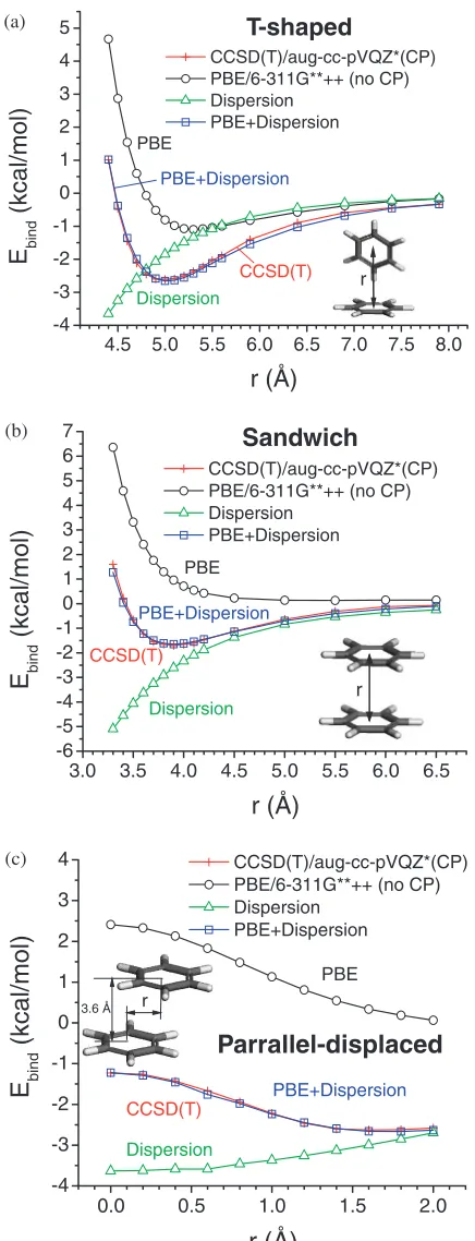
Rare gas diatomic molecules are bound through pure dispersive interactions, serving ideal benchmark systems for studying dispersive interactions with least ambiguity. We first calculated the binding energies of rare gas diatomic molecules including He, Ne, Ar, Kr, and Xe using HF, B3LYP,29) _{and PBE}30) _{methods implemented in Jaguar}31) package. Unrestricted HF and DFT methods were used with 6-311G**++ basis set and fine grid for numerical integra-tions. The basis set superposition error (BSSE) was corrected with Boys and Bernardi’s counterpoise (CP) method.32)_The large basis set and BSSE correction are necessary to minimize the numerical uncertainty in the study of these weakly bound systems. The pseudospectrum method in Jaguar was not used in order to make our parameters transferable to work with other QM packages. The calculated QM binding energies (BE) as a function of atom separation are plotted in Fig. 2 in comparison with experimental values.33,34)_{The calculated equilibrium distances and binding} energy minima are tabulated in A1 of Appendix. We found that both HF and B3LYP led to positive energy curves, indicating that there are no energy minima on the PES. PBE yielded weak bindings, but still severely underestimated the experimental BE except for Ne-Ne. On the other hand, PBE predicted too large equilibrium distance.

We optimized both the universal damping function and dispersion parameters in order to reproduce the experimental BE curves. The resulting dispersion energies (Edisp) and DFT-D energies (EDFT-D) are plotted in Fig. 2. By adding dispersion corrections, DFT-D binding energies are in very good agreement with experimental values at a wide range of separations for various rare gas dimers. The optimized parameters used in these dispersion corrections are tabulated in A2 of Appendix.

3.2 Benzene dimer

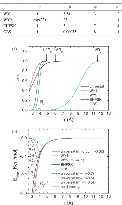
Benzene dimer is the simplest prototype system for studying aromatic – interactions that play an important role in biological systems (e.g. DNA base pairs). Benzene dimers have several typical configurations, namely, T-shaped, sandwich, and parallel-displaced configurations. The schematic illustrations of these configurations are shown in the inserts of Fig. 3. The high-levelab initioCCSD(T)35) calculations were carried out for these benzene dimers with aug-cc-pVQZ* basis set and counterpoise correction. Cou-pled-cluster theory takes into account electron correlation, thus it is capable of describing dispersive interaction accurately. These CCSD(T) results serve as references for Table 1 Parameters used in the universal damping functions that represent

various damping functions in literatures including WY1,20Þ _WY2,20Þ EHFSK,24Þ_{and OBS}25Þ_functions.

a b m n

WY1 1 3.54 3 2

WY2 expð23Þ 23 1 1

EHFSK 1 3 7 4

OBS 1 0.00075 8 1

3 4 5 6 7 8 9 10 11 12 13 0.0

0.2 0.4 0.6 0.8 1.0 1.2

r (Å) R₀

3R₀ 1.5R₀

f damp

universal WY1 WY2 EHFSK OBS 1.2R0

(a)

3 4 5 6 7 8 9 10 11 12 13 -0.3

-0.2 -0.1 0.0

0.33 0.5 0.6 0.7

Edisp

(Kcal/mol)

r (Å)

universal (m=0.33,n=-0.32) WY1

WY2 (m=-n=1) EHFSK OBS

universal (m=-n=0.7) universal (m=-n=0.6) universal (m=-n=0.5) no damping C₆/r6

1

(b)

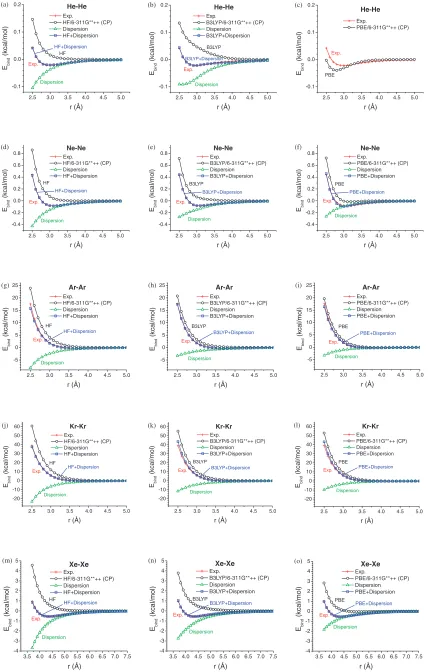
Fig. 1 (a) Optimized universal damping function [eq. (8)] and (b) dispersive correction developed in this work as well as those in literatures including WY120) _{[eq. (3)], WY2}20) _{[eq. (4)], EHFSK}24) _{[eq. (6)], and}

OBS25)_{[eq. (7)]. The same C-C equilibrium bond distanceR}

0¼3:851A˚

andC6¼425:765kcal/mol A˚6are used in all dispersion corrections for

2.5 3.0 3.5 4.0 4.5 5.0 -0.1 0.0 0.1 0.2 Dispersion Exp. HF+Dispersion Ebind (kcal/mol) r (Å) Exp. HF/6-311G**++ (CP) Dispersion HF+Dispersion He-He HF (a)

2.5 3.0 3.5 4.0 4.5 5.0

-0.1 0.0 0.1 0.2 Dispersion Exp. B3LYP+Dispersion Ebind (kcal/mol) r (Å) Exp. B3LYP/6-311G**++ (CP) Dispersion B3LYP+Dispersion He-He B3LYP (b)

2.5 3.0 3.5 4.0 4.5 5.0

-0.1 0.0 0.1 0.2 Exp. Ebind (kcal/mol) r (Å) Exp. PBE/6-311G**++ (CP) He-He PBE (c)

2.5 3.0 3.5 4.0 4.5 5.0

-0.4 -0.2 0.0 0.2 0.4 0.6 0.8 Dispersion Exp. HF+Dispersion Ebind (kcal/mol) r (Å) Exp. HF/6-311G**++ (CP) Dispersion HF+Dispersion Ne-Ne HF (d)

2.5 3.0 3.5 4.0 4.5 5.0

-0.4 -0.2 0.0 0.2 0.4 0.6 0.8 Dispersion Exp. B3LYP+Dispersion Ebind (kcal/mol) r (Å) Exp. B3LYP/6-311G**++ (CP) Dispersion B3LYP+Dispersion Ne-Ne B3LYP (e)

2.5 3.0 3.5 4.0 4.5 5.0

-0.4 -0.2 0.0 0.2 0.4 0.6 0.8 Dispersion Exp. PBE+Dispersion Ebind (kcal/mol) r (Å) Exp. PBE/6-311G**++ (CP) Dispersion PBE+Dispersion Ne-Ne PBE (f)

2.5 3.0 3.5 4.0 4.5 5.0

-5 0 5 10 15 20 25 Dispersion Exp. HF+Dispersion Ebind (kcal/mol) r (Å) Exp. HF/6-311G**++ (CP) Dispersion HF+Dispersion Ar-Ar HF (g)

2.5 3.0 3.5 4.0 4.5 5.0

-5 0 5 10 15 20 25 Dispersion Exp. B3LYP+Dispersion Ebind (kcal/mol) r (Å) Exp. B3LYP/6-311G**++ (CP) Dispersion B3LYP+Dispersion Ar-Ar B3LYP (h)

2.5 3.0 3.5 4.0 4.5 5.0

-5 0 5 10 15 20 25 Dispersion Exp. PBE+Dispersion Ebind (kcal/mol) r (Å) Exp. PBE/6-311G**++ (CP) Dispersion PBE+Dispersion Ar-Ar PBE (i)

2.5 3.0 3.5 4.0 4.5 5.0

-20 -10 0 10 20 30 40 50 60 Dispersion Exp. HF+Dispersion Ebind (kcal/mol) r (Å) Exp. HF/6-311G**++ (CP) Dispersion HF+Dispersion Kr-Kr HF (j)

2.5 3.0 3.5 4.0 4.5 5.0

-20 -10 0 10 20 30 40 50 60 Dispersion Exp. B3LYP+Dispersion Ebind (kcal/mol) r (Å) Exp. B3LYP/6-311G**++ (CP) Dispersion B3LYP+Dispersion Kr-Kr B3LYP (k)

2.5 3.0 3.5 4.0 4.5 5.0

-20 -10 0 10 20 30 40 50 60 Dispersion Exp. PBE+Dispersion Ebind (kcal/mol) r (Å) Exp. PBE/6-311G**++ (CP) Dispersion PBE+Dispersion Kr-Kr PBE (l)

3.5 4.0 4.5 5.0 5.5 6.0 6.5 7.0 7.5 -4 -3 -2 -1 0 1 2 3 4 5 Dispersion Exp. HF+Dispersion Ebind (kcal/mol) r (Å) Exp. HF/6-311G**++ (CP) Dispersion HF+Dispersion Xe-Xe HF (m)

3.5 4.0 4.5 5.0 5.5 6.0 6.5 7.0 7.5 -4 -3 -2 -1 0 1 2 3 4 5 Dispersion Exp. B3LYP+Dispersion Ebind (kcal/mol) r (Å) Exp. B3LYP/6-311G**++ (CP) Dispersion B3LYP+Dispersion Xe-Xe B3LYP (n)

3.5 4.0 4.5 5.0 5.5 6.0 6.5 7.0 7.5 -4 -3 -2 -1 0 1 2 3 4 5 Dispersion Exp. PBE+Dispersion Ebind (kcal/mol) r (Å) Exp. PBE/6-311G**++ (CP) Dispersion PBE+Dispersion Xe-Xe PBE (o)

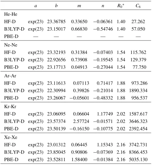
our dispersion corrections. The CCSD(T) calculations found that the parallel-displaced and the T-shaped configurations were almost energetically degenerate, and more stable than the sandwich configuration by 0.93 and 0.91 kcal/mol, respectively (see Table 2). This can be understood since the C-H electrostatic interactions dominate in the T-shaped

configuration, whereas the weaker dispersive interactions dominate in the sandwich configuration. The electrostatic and the dispersive interactions coexist in the parallel-displaced configuration.

We calculated the binding energies of benzene dimers for all three configurations using DFT-PBE method implement-ed in Jaguar since our calculations on rare gas diatomic molecules show that PBE performances the best in describing dispersion among the studied methods. The 6-311G**++ basis set and fine grid were used in the PBE calculations. Counterpoise correction was not included in this case because the CP correction is not practical for large systems, and we want our dispersion parameters to be applicable to most routine DFT calculations. The pseudospectrum method inJaguarwas not used for parameter transferability. Figure 3 shows the PBE binding energies together with the CCSD(T) results for comparison. As seen from Table 2, PBE severely underestimated the binding energies for the T-shaped and sandwich configurations compared to the CCSD(T) results. The equilibrium distances calculated by PBE were too long. No energy minimum was found on the PES of the parallel-displaced configuration.

With a single set of parameters in the dispersion corrections, our PBE-D reproduced the CCSD(T) results well for three different configurations at a wide range of separations as shown in Fig. 3 and Table 2. These config-urations of benzene dimers exhibit distinct binding character-istics changing from dispersive to electrostatic interactions, thus they serve as good test cases to examine the trans-ferability of the dispersion parameters. Table 3 lists the optimized parameters used in the dispersion corrections with the universal damping functions.

During the least square fitting process we started from the WY2 damping function [a¼expð23Þ, b¼23, m¼1 and n¼1], and optimized six parameters simultaneously, name-ly, a,b,m,n andC6 forC andH. The resulting optimized

damping parameters are a¼expð23Þ, b¼23:01434, m¼

0:33360andn¼ 0:31952. Themandnare about 1/3 of the

initial values, whereasa andbchange little. This optimized universal damping function and corresponding dispersion corrections are plotted in Fig. 1(a) and 1(b) in comparison with those used in literatures. As shown in Fig. 1(a), the optimized universal damping function starts to decay (fdamp¼0:99) atr¼1:5R0. For comparisons, WY1, WY2

and EHFSK functions were designed to decay atr¼1:2 R0.

OBS function starts to decay at r¼3R0. The slope of the

universal damping function is similar to that of OBS function, but smaller than those of WY1, WY2 and EHFSK functions. From Fig. 1(b), we found that the dispersion Table 2 Equilibrium distances (Rmin) and binding energy minima (Emin) of

benzene dimers calculated using PBE methods and its dispersion correction (PBE-D).Rminhas a unit of A˚ ,Eminkcal/mol.

T-shaped sandwich parallel-displaced

Rmin Emin Rmin Emin Rmin Emin

CCSD(T) _{5.0 2:610 3.9 1:700 1.6 2:630}

PBE 5.3 1:100 5.5 0.129 — —

PBE-D 5.0 2:656 3.9 1:644 1.8 2:667

_{ab initioQM data are taken from Ref. 35).}

4.5 5.0 5.5 6.0 6.5 7.0 7.5 8.0

-4 -3 -2 -1 0 1 2 3 4 5

Dispersion

CCSD(T) PBE+Dispersion

E

(kcal/mol)

r (Å)

CCSD(T)/aug-cc-pVQZ*(CP) PBE/6-311G**++ (no CP) Dispersion

PBE+Dispersion

T-shaped

PBE

r

(a)

3.0 3.5 4.0 4.5 5.0 5.5 6.0 6.5

-6 -5 -4 -3 -2 -1 0 1 2 3 4 5 6 7

Dispersion CCSD(T)

PBE+Dispersion

E

(kcal/mol)

r (Å)

CCSD(T)/aug-cc-pVQZ*(CP) PBE/6-311G**++ (no CP) Dispersion

PBE+Dispersion

Sandwich

PBE

r

(b)

0.0 0.5 1.0 1.5 2.0

-4 -3 -2 -1 0 1 2 3 4

Dispersion CCSD(T)

PBE+Dispersion

E

(kcal/mol)

r (Å)

CCSD(T)/aug-cc-pVQZ*(CP) PBE/6-311G**++ (no CP) Dispersion

PBE+Dispersion

Parrallel-displaced

3.6 Å r (c)

correction using the universal damping function behaves similarly to that using WY1 function, even though the fitting started initially from the very different WY2 function. To conform the possibility of this transition, we examined the behaviors of universal damping functions by varying m (¼ n) from 0.7, 0.6, to 0.5 while fixing a¼expð23Þ and b¼23. These universal damping functions are plotted as dashed lines in Fig. 1(b). We indeed observed the gradual changes from WY2 to the universal function when m decreases. Our optimization results are consistent with the conclusion of Wu and Yang20)_{that the soft damping WY1} is better than the hard damping WY2. Our optimized damping function has a different function form but a similar effect as WY1 on dispersion corrections at the studied range. Wu and Yang found the better damping function by comparing two fixed functions. In this work, we obtained the similarly behaved damping function naturally through optimization.

4. Conclusions

Designing a good damping function is critical in develop-ing a successful empirical dispersion corrected DFT method. We here propose a universal damping function that unifies different damping functions that have been used in liter-atures. By implementing the single universal function, one can examine and compare the performances of various existing DFT-D methods at an equal footing. Moreover, the flexibility of the universal function allows further optimization of damping functions, e.g., a smooth change of the softness of damping. The optimization of damping function is not only a mathematical obligation but also an estimation of missing dispersive interactions in DFT methods. It is possible to design a variant of the universal damping function by imposing additional physical con-straints. Applying dispersion corrections on DFT using the optimized universal damping functions, we can describe dispersive interactions accurately for rare gas diatomic molecules and benzene dimers. It is straightforward to develop parameters for other atom types in different chemical environments.

Acknowledgments

We acknowledge the supports from ARO (W911NF-05-1-0345) and ONR (N00014-05-1-0778).

REFERENCES

1) P. Hohenberg and W. Kohn: Phys. Rev. B136(1964) B864. 2) W. Kohn and L. J. Sham: Phys. Rev.140(1965) 1133. 3) S. Kristyan and P. Pulay: Chem. Phys. Lett.229(1994) 175. 4) J. M. Perezjorda and A. D. Becke: Chem. Phys. Lett.233(1995) 134. 5) M. P. Waller, A. Robertazzi, J. A. Platts, D. E. Hibbs and P. A.

Williams: J. Comput. Chem.27(2006) 491.

6) P. Hobza, J. Sponer and T. Reschel: J. Comput. Chem.16(1995) 1315. 7) H. Y. Jeong and Y. K. Han: Chem. Phys. Lett.263(1996) 345. 8) E. J. Meijer and M. Sprik: J. Chem. Phys.105(1996) 8684. 9) W. Kohn, Y. Meir and D. E. Makarov: Phys. Rev. Lett.80(1998)

4153.

10) A. Hesselmann and G. Jansen: Chem. Phys. Lett.367(2003) 778. 11) Y. Zhao and D. G. Truhlar: Phys. Chem. Chem. Phys.7(2005) 2701. 12) X. Xu and W. A. Goddard: Proc. National Academy Sci. U.S.101

(2004) 2673.

13) A. D. Becke and E. R. Johnson: J. Chem. Phys.127(2007) 154108. 14) Y. Zhang, X. Xu and W. A. Goddard: Proc. National Academy Sci.

U.S.106(2009) 4963.

15) M. Dion, H. Rydberg, E. Schroder, D. C. Langreth and B. I. Lundqvist: Phys. Rev. Lett.92(2004) 246401.

16) A. Puzder, M. Dion and D. C. Langreth: J. Chem. Phys.124(2006) 164105.

17) O. A. von Lilienfeld, I. Tavernelli, U. Rothlisberger and D. Sebastiani: Phys. Rev. Lett.93(2004) 153004.

18) A. Tkatchenko and O. A. von Lilienfeld: Phys. Rev. B 73(2006) 153406.

19) R. Ahlrichs, R. Penco and G. Scoles: Chem. Phys.19(1977) 119. 20) Q. Wu and W. T. Yang: J. Chem. Phys.116(2002) 515.

21) J. Antony and S. Grimme: Phys. Chem. Chem. Phys.8(2006) 5287. 22) S. Grimme, J. Antony, T. Schwabe and C. Muck-Lichtenfeld: Org.

Biomol. Chem.5(2007) 741.

23) P. Jurecka, J. Cerny, P. Hobza and D. R. Salahub: J. Comput. Chem.28 (2007) 555.

24) M. Elstner, P. Hobza, T. Frauenheim, S. Suhai and E. Kaxiras: J. Chem. Phys.114(2001) 5149.

25) F. Ortmann, F. Bechstedt and W. G. Schmidt: Phys. Rev. B73(2006) 205101.

26) U. Zimmerli, M. Parrinello and P. Koumoutsakos: J. Chem. Phys.120 (2004) 2693.

27) F. London: Z. Phys. Chem. Abt.B11(1930) 22.

28) M. J. Buehler, A. C. T. van Duin and W. A. Goddard: Phys. Rev. Lett. 96(2006) 95505.

29) A. D. Becke: J. Chem. Phys.98(1993) 5648.

30) J. P. Perdew, K. Burke and M. Ernzerhof: Phys. Rev. Lett.77(1996) 3865.

31) Jaguar, version 7.0, Schrodinger, LLC, New York, NY, (2007). 32) S. F. Boys and F. Bernardi: Mol. Phys.19(1970) 553. 33) J. F. Ogilvie and F. Y. H. Wang: J. Mol. Stru.273(1992) 277. 34) J. F. Ogilvie and F. Y. H. Wang: J. Mol. Stru.291(1993) 313. 35) M. O. Sinnokrot and C. D. Sherrill: J. Phys. Chem. A108(2004) 10200. 36) A. K. Rappe, C. J. Casewit, K. S. Colwell, W. A. Goddard and W. M.

Skiff: J. Am. Chem. Soc.114(1992) 10024. 37) A. Bondi: J. Chem. Phys.68(1964) 441.

Table 3 Parameters used in the dispersion corrections for benzene dimers in this work. PBE-D represents dispersion corrections on a PBE method.R0has a unit of A˚ ,C6kcal/mol A˚6.a,b,mandnare dimensionless.

C H

a b m n R0 C6 R0 C6

PBE-D expð23Þ 23.01434 0.33360 0:31952 1.9255 425.747 1.4400 5.487

Appendix Table A2 Parameters used in the dispersion corrections for rare gas diatomic molecules (He, Ne, Ar, Kr and Xe) in this work. HF-D, B3LYP-D and PBE-B3LYP-D represent dispersion corrections on HF, B3LYP and PBE methods. R0 has a unit of A˚ , C6 kcal/mol A˚6. a, b, m and n are

dimensionless.

a b m n R0 C6

He-He

HF-D expð23Þ 23.36785 0.33650 0:06361 1.40 27.262 B3LYP-D expð23Þ 23.15017 0.66830 0:54746 1.40 57.050

PBE-D — — — — — —

Ne-Ne

HF-D expð23Þ 23.32193 0.31384 0:07403 1.54 115.762 B3LYP-D expð23Þ 22.92656 0.73908 0:19545 1.54 129.379 PBE-D expð23Þ 23.17713 0.04913 0:27044 1.54 77.750

Ar-Ar

HF-D expð23Þ 23.11613 0.07113 0.71417 1.88 973.286 B3LYP-D expð23Þ 22.30994 0.39826 0:21014 1.88 1890.334 PBE-D expð23Þ 23.26067 0:05601 0:48332 1.88 956.537

Kr-Kr

HF-D expð23Þ 23.06095 0.06604 1.17749 2.02 1587.617 B3LYP-D expð23Þ 23.57374 2.57724 0:01571 2.02 3646.323 PBE-D expð23Þ 23.50139 0:16150 0:10775 2.02 2392.454

Xe-Xe

HF-D expð23Þ 23.01312 0.06445 1.15343 2.16 3742.731 B3LYP-D expð23Þ 23.85045 0.90806 0:07369 2.16 8366.453 PBE-D expð23Þ 23.52811 1.58400 0:01384 2.16 5035.130

_{vdW radii are taken from Ref. 37).} Table A1 Equilibrium distances (Rmin) and binding energy minima (Emin)

of rare gas diatomic molecules (He, Ne, Ar, Kr and Xe) calculated using HF, B3LYP and PBE methods as well as their corresponding dispersion corrections (HF-D, B3LYP-D, and PBE-D).Rmin has a unit of A˚ ,Emin

kcal/mol.

He-He Ne-Ne Ar-Ar Kr-Kr Xe-Xe

Rmin Emin Rmin Emin Rmin Emin Rmin Emin Rmin Emin

Exp. _{3.0 0:022 3.10:084 3.8 0:283 4.0 0:400 4.4 0:559}

HF — — — — — — — — — —

HF-D 3.0 0:021 3.10:086 3.8 0:281 4.0 0:391 4.4 0:549

B3LYP — — — — — — — — — —

B3LYP-D 2.9 0:022 3.10:083 3.7 0:284 4.0 0:397 4.3 0:557

PBE 2.8 0:040 3.20:015 4.1 0:088 4.7 0:033 5.10:046

PBE-D — — 3.00:095 3.8 0:297 4.0 0:394 4.40:553