THr AEnoNAUTTcAL ]ounxnr
Apru12001
ABSTRACT
A m e t h o d i s p r o p o s e d by which a direct numerical simulation of the c o m p r e s s i b l e N a v i e r - S t o k e s equations may be embeddecl within a more general aeronautical cFD code. The methocl rray be applied to a n y c o d e w h i c h s o l v c s the Euler eqLrations or the Favre-averagecl N a v i e r - S t o k e s e q u a t i c l n s . A f b r m a l d e c o m p o s i t i o n of the flowfielil is L r s e d t o d e r i v e m o d i f i e d equations tor use with direct numerical sim-L r l a t i o n s o l v e r s . S o m e p r e l i m i n a r y applications fbr model flows with t r a n s i t i o n a l s e p a r a t i o n bubbles are given.
1 . 0 IN T R O D U C T I O N
Applied careful ly. aeronauticul cornpr-rtational f-luicl dynamics (cFD)
codes can deliver usefirl predictions of flow aroun<J aircrafi. The
r.nethods generally work well when the f-low is fLrlly tLrrbulent ancl
rcmains attached to the surface. The standard rnethods work much
less well when transition to turbulcnce must be taken into accollnr or
when the turbulenr flow is subjected to rapicl changes in the imposed
strain field. The rnodels are particularly challengecl in regions where
I'low scperration or reattachment takes place. By contrasl direct
nr_r-merical simLrlations (DNS). whereby the governing equations are
solved in full, are too expensive fbr complete calcujations of flows
with aeronar-rtical application, but can deliver accurate solutions of
simpler problems withoLrt modelling errors. The range of problems
that can be tackled by DNS is increasing as the po*.r of computers
increases and DNS and the relatecr approach o1'large-edcly
simula-tion (LES) are bein-e applied to more ancr more complex -eeomerries
and f-low fieldstr-r). The ob,jective of the current research is to link
the two apprcaches by providing a framework whereby an
aeronauti-cal cFD code can provide the context fbr a iletailed DNS. which in
turn can automatically f'eedback improved physical modellin-r of
Iocal phenomena to improve the quality of the overall prediction.
As a model problern we consider thc case of a separation bLrbble.
irritially laminar. but undergoing transition to turbulence ancl
reattaching as a turbulent boundary layer. In high lift confi-surations
sLrch bubbles rnay form on the slat and a failure of the flow to
reattach ultirnately causes stall of the configuration. prediction of the
conect flow with conventional cFD is irnpossible as typically a
tran-sition point must be flxed close to the location where separation
takes place, in order to get a convergecl resr-rlt. However this fix
r93
Embedded
direct numerical
simulation
for
aeronautical
CFD
N . D . S a n d h a m , M . A l a m a n d S. Morin S c h o o l o f E n g i n e e r i n g S c i e n c e s U niversity of Southampton S o u t h a m p t o n , U K
precludes calculation of the maximum lifi coefficient. a quantity
fbr-which accurate predictions at'e essential i1'clesign is to be optirnised.
Several direct simulations of complete separation bubbles hlve
been carried out recently. These simulations include the larninar
sep-aration, transition process. turbulent reattachment. and relaxation o1,
the turbulent boundary layer downstrearn of reattachment. Spalart
and Streletstat specified a fiee stream normal velocity profile and
simr-rlated a bubble with a length of approxirnately 300 tirnes the
momentum thickness at separation. Alam and Sandhllnr5r 11secl o
sirnilar Inethod fbr prescribing the fl'ee stream velocity distribLrtion
but focLrsed on shorter br-rbbles with lengths of the order of 40 times
the momentum thickness at separation. The bubble phenomena
reproduced in these simulations closely match earlier experintental
work. Besides providin_u data firr understanding flow instability
mechanisms (Alam and Sandham). comparisons with aergnaLrticiil
codes (Spalart and Strelets) and turbLrlence rnodelling (Hatlzic alti
Hanjalictot, Howard et ultl)) the simr-rlations also demonstratc the
f-ea-sibility of simr-rlating flow phenomena at realistic Reynolds numbers
on modern computers. It is therefbre f-easible computationally to
consider a direct simulation of a slat separation bubble (which may
only occupy lc/c of chord) and a simultaneous CFD simulation of the
rest of the f'low. The problern which we attempt to adclress in the
present work concerns the details involved in coirplin-u the twcr
approaches. In Section 2.0 we present the governing equation ancl their
Favre-averaged counterparts. such as mery be usecl in cFD cocles. In
Section 3.0 we introduce a f-low decomposition techniqtre using thc
Euler equations and the Favre-averaged equatior-rs as examples. This
technique is then applied in Section 5.0, usin-e clirect simulation
numerical methods given in Section 4.0. Finally in Section 6.0 we
present results fiom a calculation using a Favre-averagecl base f1ow.
All the equations and exanrple are presentecl fbr compressible 1low.
2.0 GOVERNING
EQUATIONS
2.1 Instantaneous
equations
The governing equations fbr mass, momentllnt and energy conserva_
tion ntay be written in Cartesian tensor notation as:
February 2000, accepted l8 Januarv 2001.
194
THE AenoNAUTrcAL lounNar- A p r u 1 2 0 0 1( l o t
t l l r
( l2 )
( r 3 )
( 1 4 )
l p t ( p r r , ) n 6t i.r,
r 1 ( p r r , ) ,
? ( P u 1 t , )
_ C p
;
-8t d.t, 6,t,
t ) = ( y - l ) p e
with y the ratio of specfic i s N e w t o n i a r n a n d f o l l o w s
( l )
Arii
d t ,
heats. Aclditionally we asslrme that,n. tj,1Li
Fourier's law for heat conduction:
d r , 2 A D , ' *
)
- r - - - - | ) i i
I
0 r , 3 0 r ^ " )
( 2 )
_ | C u ,
T , , : L l l
r l . l l
\ c'{i
a n d w e h a v e a s s u m e d th a t
I E , c [ ( 6 , + p ) t r , ] ? q , , ? ( ' c , , t t , )
T
-Ar Ar d-r, 6-r,
where Er = p @ + t/zLt1t), e bein-e the irlternill energy. The fluid is
assumed to fbllorv the perf'ect gas law with constant snecific heats
( 3 )
. . . ( b )
where pt is the viscosity, -uiven by apower law tirnctictn of
tempera-ture, ancl r is the thermal condr-rctivity. The Euler eqr-rations arise
when the terms involving viscclsity and thermal condr"rctivity are
dropped fiom the right hand sides of Equations (2) and (3).
2.2 F avre-averaged equations
In Navier-Stokes calculations with a turbulence rnoclel a flow
decomposition into an average and a f-luctuuting conrptlnent is used.
For the compressible equations considered here. a convenient tbrrn
which preserves the original structure of the ecluations is thc Favre
method of mass-wei-qhted variables defined according to
u = i , + t t ' , ' p = p + p '
T - - 7
+ 7 "
t : - f - + F - ' " r " I
p = p + p '
w h e r e i , = p u , / p a n d w e c a n a l s o w r i t e E , = p E w i t h E = E + E " .
lt shoLrld be noted that fbr anv function l:
F o r l o w M a c h n u m b e r f l o w s t h e F a v r e d e c o m p o s i t i o n r e d u c e s to t h e L r s u a l R e y n o l d s - a v e r a g e c l f o r m o f t h e e q u a t i o n s .
T h e F a v r e - a v e r a s e d m a s s c o n s e r v a t i o n e u u r " r t i o n i s
I
T h e m o m e n t L l l n e q u a t i o n s a r e :
T I r c l e r r n s , i . pu,, ,'t.p,qr1, ,,td pi,- .,,,, hc rnodelletl
by vr. ui. \,-r (e u,le.r,). \,r tiA/i.r, ) and v r (ieli.r,;
respectively (see Vy'i lcoxtst).
3.0 A DECOMPOSITION
APPROACH
The basic idea of the present contribLrtion is to perfirrm a direct
numericitl simulation fclr phenonrena such as transition and
turbu-lence r-rsing as base flows solutions nhich mar arise fiom standard
aeronautical CFD calculations of cornpressiblc flow. A conceptr-rally
sirnple way of arran-uin-e this is to consider tlie total flow to be a
superposition of a known base flow and an unknou n tinte-dependent
perturbation fiomthis to be deterntined bv direct nunterical
simula-tion. In the fbllowing subsections we derir e the relevant eqLrations
for a base flow which satisfies either the ELrler equations or the
Favre-averaged eclr-rations firr turbulent flori. Sintilal br-rt sirnpler
ecluations can be derived fbr incompressible f-lou.
3.1 Euler base flow decomposition
As a first example of the techniqr-re we consider a clecorlpositit'rn
into an Er-rler component p,'.tii', Ei: which is iisslrrned to have been
computed from a separate Euler solver, and a der iation li'ont this
which we label pt,.t/1. Ef). Insertin-e this clecornprosition into the
-rov-ernin-9 equations and subtracting the ELrlcr solution of the equations
l e a d s t o t h e fo l l o w i n g e c l u a t i o n s . F o r c o n t i n u i t y u c h a r e :
T h e e n e r g y e q u a t i o n b e c o m e s
- F - ^ . , 7
i E , , i l ( E , + F ) n l * a E
-?t
e,r,
cl:.r
a ( , - , , | , , , , , \ ( ^ ( p t " t t " ) * ; _
[ 4 , , , , , * u i p u i u -
) P u , u I t - ' l
^
- - , r \ / . l ( . \
T h e m o m e n t u r n e q u a t i o n b e c o m e s :
i ) .
t (
_ - r - L P r r i | | r cI cxi
t E r D l T l '
. t ' , , o . t t t t i t ' l ) " ' t i i ( ' r ( D t l ' , - D ' / i , ) ' = i F
-| '
,^,,, t-:r, ,tt, i:v,
i l t r l t
r
-i.r
(-5 )
/ ^ \
l ? u c l t , 2 ? . u ^ I
T - r r l ' - !
r , , - l r | | v I
" I l r i . v , I i . r , " )
\ / r ^ /
( ' l 4 i = - l ( ^
cti
I li,'
( 7 )
( u )
t = o l
7 = o l
a p l ( p D l ) n
SaNnsav ET AL
and the energy equation is:
A r D A
? * .
[ 1 6 r ' + p o 1 u ,
ot oxi
6 r l , t '
, 0 1 r l u , )
r
-Ar,
tr,
where
+ ( E f + p E ) u l 1 =
Evngnoen DIRECT NUMERICAL sIMULATIoN FoR AERoNAUTTcAI cFD
195
,
( e,,,o attl 2 cri - )
T u = f . l l 1 + . - ^ ^ : 0 , , 1
\ c.r, c_ri J a.rr )
p o = ( p r ' - p o r u ) ( y - l )
. . r i \
, r [ r t t , t t , t t o t , ? " . I
, u = ; l n ' - p o ( e u
* T ' , - r t r t t i l i + , , i , , !
l l
3.2 Favre base flow decomposition
A similar procedure leads to equations fbr the f'low-fielcl p,t.,,,,'. Elt
computed as a perturbation fiom a Favre-averaged base flow pi',r|. E.f. . For the continuity equation we have:
4 . 0 N U M E R I C A L
M E T H O D
F O R D N S
The new formulations of the governing equations for mass,
momen-tum and energy given in Section 3.0 are solved numerically using
techniques that are suitable fbr efficient calculation of f'lows with a
wide range of length and time scales. Time discretisation is achieved
with an explicit low-storage third-order Runge-Kutta scheme. The
time step is fixed to be well within the stability limit to ensure
tem-poral stability. Spatial discretisation is by means of compact
pacld-type high order schemes with ave-point stencil on the right hand side
and a three point stencil on the lefi hand side. These rnethocls require
only a tridiagonal matrix solver. They achieve sixth order accuracy in the inner part of the domain, reducing to third order at boundaries
and have good wave resolution properties (Leleror;.
Non-ref'lecting characteristic boundary conditions are useiJ at the
in f-low and outf-low boundaries. The methods used at the outf'low
were originally proposed by Thompson (19137) and invorve
criagonal-ising the Euler equations and zeroing out the rows containing
char-acteristic velocities that are pointing inwards into the computational
domain. At the in flow boundary we use a modification to this
approach fiom Sandhu and Sandham(tot whereby the basic inflow is
fixed but with the outgoing characteristic added by integrating it
along with the rest of the Navier-Stokes equations. This provides a
rnethod of fixing an inflow condition while allowing souncl waves to
pass smoothly through the inflow boundary. For Navier-Stokes
cal-culations a boundary-layer profile is needed at the infrow. This is
found fiom a similarity solution of the compressibre raminar
bound-ary-layer equations.
No slip conditions are used fbr the lower boundary to simulate a
smooth surf'ace. A mixed set of boundary conditions are used at the
upper boundary to maintain the flow fleld. A non-reflecting
charac-teristic boundary condition is used for density and a zero vorticity
boundary condition is implemented by settin-q
; l ) ^ I )
c't I - c\J"
o.y' d,r
and we set
u D = 0
. (24)
r ? 5 r
It should be noted that the boundary conditions specil'ied here need
not be the same as those used fbr the base flow calculation which is
one of the strengths of the decomposition method. In the examples in
this paper we use Dirichlet conditions fbr the base f-row and mixed Neumann-Dirichlet conditions fbr the full simulation. Alternative ways of specitying the upper boundary are currently under review to
fully utilise the flexibility off-ered by the decomposition approach.
For all the simulations presented in the fbllowing two sections the
computational box lengths are l0b* in the wall-normal direction and
120b" in the streamwise direction where 6" represents the
displace-ment thickness of the incoming boundary layer. The grid is stretched
in the wall-normal direction to cluster more points in the boundary layer. The number of grid points used were 140 in the wail-normal
direction and 100 in the streamwise direction. For viscous
calcula-tions the Reynolds number was fixed to be -500. the prandtl number
to 0.72, and viscosity varied i1s 1,1 - f t)67.
5 . 0 E U L E R - D N S
S I M U L A T I O N
O F A
SEPARATION
BUBBLE
The first step in producing a simulation is to compute an Euler
solu-tion. In the anticipated applications this would conre from a standard
aeronautical Euler solver. Here we consider simpler rnodel problerns
to demonstrate the techniqr-res. An external velocity profile which
can be used to produce a separation bubble is
. ( t 6 )
. . . ( 1 8 )
. (20)
a ,r)
c'P c' , rr
- - + . ( p r r i + p ' u !
7 = g
CI C-T,
The momentum equation is:
a / l ) ,
. ' ( p r l , ) C I _ ^
#
CI+ - " - lptr,D
C.T,l t r l + , , i i l +
a F . ^ n t D n l - - - - i - i i t " ' ( 1 9 )
@tt?
+ po,,o,
' ') !!.- = - ry- *!- *
o\Ptt'tr'
)
A-r., 6-t, 0-,, 6, ,
and the energy equation becomes:
+.3
6 t d r , "t,r.' + pD
t)tt,
+ (Ef + pF
)u?1=
t D ^
o0, c
- ; : 1 - "
f t l u
, + 'i u l )
c.r, o.ri^ t - - r - - t F
n
n , l- t , , t t " , + u , p t t ' , u " , I - p u ' . i r " , u " , + y p e " i ' ,f
where
n ? u ! C u l 2 ? u ! T ; = F ( . + ^ - ; ^ - - d , , )(--r,
c.I; J r:r{
p ' = ( p u ' - p , u o ' X y - l )
')l
n o
= ! l u " - o'( ,
p L
\
' ' ' ( 2 1 1
r ) ) r
. (23)
, , / D I )
f - I t , I t i ) t l u ; u , n + l - n ' I
196
U(.r) = A - B TanhlC(.r - D)l (26\
w h e r e A . B , C a n d D a r e c o n s t a n t s . w h i c h c a n b e f i x e d t o d e t c r n l i n e t h e r a t c a n c l s i z e o f t h e d r o p i n l r e e s t r e a n t v e l o c i t y . F o r t h e s i m t t l a -t i o n s i n -t h i s s e c -t i o n w e L -t s c A = 0 ' 9 1 . B = 0 0 9 . C = 0 ' 0 u a n d D = 4 0 . w h i c h l e a c l s t o a f l ' e e s t r e a m d r o p o f 1 8 % c o n f i n e d w i t h i n t h e d o m a i n .
W e c o m p u t e t h e b a s e E , u l e r f ' l o w f o r t h i s s i r n p l e c a s e b y s o l v i n g t h e f u l l c o m p r e s s i b l e p o t e n t i a l e q u a t i o n
, t , - , , . ' . ' , r r - ' - l d - Q , ' - Q _ I l f c Q ), ' - Q I t a I r ' Q I
^ . - r ^ - - " l { - ^ l ^ ' - l - l ^ - 1
( y - ( ' y - r t - [ \ r l r l ( i r - \ r ' y l , ' y - _ ]
. . . ( ) l l
2 eb
a0 a-0
f t ^ ^
-ct- ox cy cxcy
r , v h c r e t h e s o r , r n d s p e e d a i s f i x e d r e l a t i v e t o s t l t g n r t i t t l t c o n d i t i o n s a . b y
2 C 4 C b
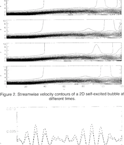
Streamwise velocity contours of a 2D self-excited bubble at
different times.
[image:4.612.332.575.87.371.2] [image:4.612.52.299.560.732.2]T i m e
Figure 3. Time history oJ a wall normal velocity at various heights
s h o w i n g u n s t e a d y s h e d d i n g .
There havc been susl-ricions in the past that shedtlirtg tttav be
trig--Uerc-d nunterically so it is rtsel'ltl to havc pt'eclictiotls ol' tltc slttllc
phcnotlena witlr c()ntpLlter progrilnrs that use clil'lcrcrtt rttcthttcls.
Fig-ture rl shows the tinre avcraged bLrbble. Scpanttetl I'lori is fttttttcl fitr
- 5 0 < . r < 7 0 .
6.0 EXAMPLE
OF FAVRE-DNS
SIMULATION
F o r t h e s i n r u l l t i o r - r s in t l - r i s s c c t i o n \ \ c u \ L - . 1 = ( ) ' t ) - 1 . l l = 0 ' 0 ( t . C = 0 . 0 U a n d l ) = : 1 0 . w h i c h l e a d s t o a f t ' c - c \ t r c r t r l l d r o p o l ' l l % c o n -f i n c d w i t h i n t h e d o m a i n . T h i s r e s u l t s in a n u r g i n r L l l r - s c p u r u t e c l f l o u ' a n d w c a p p l y t i r r c i u - u a t t h e i n l - l o $ ' t o t r i g g c l ' t h c \ o t ' t e r s l l e d d i n g i n a c l e t e r m i n i s t i c w a y . T h e f o r c i n - s is g i v e n b r
s ' = 4 , . 1 ( . r ' ) S i n ( t ' r r ) . . . ( 1 9 )
w l r e r c /(r') is it norrlalisccl f'r-rnciton o f .r uitlt rt Ittrlritt'tttt.tt r a l t t c o f u n i t y a r , d a p e a k i l t - \ ' = I w i t h t h e c t ' r l l s t a t l t \ \ e l . l \ , , = ( ) ' 0 1 - 5 a t l c l t ' r =
0 . 1 2 .
T o g e n c r a t e a F a v r e b a s c l ' l o w u ' e f i r : t o 1 ' r i l l n r n r L n E L t l e t ' c l e c o t t . t -p o s i t i o n c a l c u l a t i o n t i r r t l t e -p r e s c r i b c c l [ l ( ) t c n t r i . r ] I ' l r r r t . [l c : t t l t s l k r r t t t h i s c a l c r r l l t t i t l n a r e s h o w n o l l F i g ' 5 ' A g a i r l u c ' ] l ' t t ' \ ( ) l . l c \ s h e t l d i n g ' b u t t h i s t i n t e i t i s r c g u l a r a n c l p r e c l i c t a b l c . l - h c r . c . t L l l . t r ( ) n t tl t i s s i t t t t t -l a t i t -l t -l a r e t h e t -l a v c r a g e c -l o v e r o l l e c v c l c t l l ' t l l e 1 r ; 1 ' i . , r ' 1 1 ' s h c t l c l i t l g t t l c l c t e n t r i n e tl r e I - - a v r c - l r v e r a g e c l n t e a n l n c l l ' l L t e t t L . t l t , ) n t a l ' l l \ . r \ t t h i s -p o i n t w ' c h a v c t h e s t a t i s t i c l l l e r l u i v r t l e n t o l ' i t . r L l . L t l . r l i l t t i r l t l l c F a r " r c
-Tu l, AEnoNAUTICAI Tounxal Aprul 2001
F i g u r e 2 .
( ao
)'l
T l ^ I 1
\ d v l ]
0 - - - t l ^ ( 2 8 )
A t t h e s u b s o n i c M a c h n u m b e r s u s e d h e r e t h e r i g h t h a n c l s i d e o f E q u a t i o n ( 2 7 ) i s s u f f i c i e n t l y s r - n a l l t h a t i t e r a t i r , ' c n u t l e r i c u l m e t h o c l s s L r i t a b l e f o r L a p l a c e ' s e c l u u t i o n s t i l l c t t n v e r ' - u c . W e t t s e a s t r a i Q h t f b r -w a r d G a u s s - S e i d e l p r o c c d u r e b a s e d o n s e c t t n c l - o r d e r f i n i t e d i t t c r -c n -c e s . T h e s o l u t i o n i s t h e n i n t e r p o l a t e -c l o n t o t h e a -c t l l a l m e s h t t l b e L r s e d i n t h e d i r e c t n u m c r i c a l s i m u l a t i o n s .
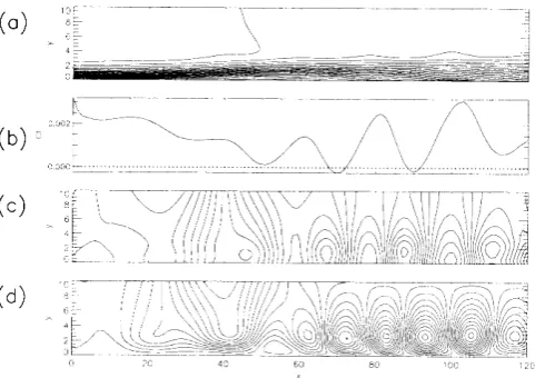
T h e s i m u l a t i o n u s i n g t h e E u l e r b a s e 1 ' l o w d e c o t n p o s i t i o n l l ' o t l l S e c t i o n 2 . 1 w a s r l l n u p t < t t i t n e / = , 5 0 0 . I n s t a n t a n e t ) L l s s n a P \ h ( ) t s () f t h e t c r t a l v e l o c i t l , f i e l d ( i . e . u = u t ) + r r l l ) ti r r t t a n c l t' a r e s h t l w n o n F i g . I ( a ) a n d ( d ) t o - s e t h e r w i t h t h e s t r e u m w i s e v a r i a t i o n o f s k i n l l ' i c t i o n ( b ) and the pressure field (c). It can be seen that there is an Llnsteady s e p a r a t i o n b L r b b l e w i t h w e a k n a t t t t ' a l v o r t e x s h e d d i n - e fr o r n b e h i n d t h e b u b b l e . A t i r n e s e r i e s o f t h e s l i e d d i n g . a s i t a p p e a r s in t h e s t r e i l n l -w i s e v e l o c i t y f i e l d i s s h o -w n o n F i - s . 2 . T h e r e s l t l t t h a t t h e r e i s v o t ' t e x s l r e d d i n g f i r r t h i s o w c o n c l i t i o n i s c o n s i s t c n t w i t h t l i e e a r l i e r s i t n u l i i -t i o n o l ' R i s -t e r r 1 1 ( l l ) . A d d i t i o n a l l y t i n r e s e r i e s n r e i - r s L r r c n r c n t s f r o t - t - t w i t h i n t l i e s h e d d i n g r e - e i o n (F i - s . 3 ) s h o w i t s h e c l d i n g in t l . r e f i r r r t l o f w a v e p a c k e t s w h i c h i s a l s o c o n s i s t e n t w i t h t h e p r e v i o t - t s fi n c l i n g s .
( o l
( b )
( . )
( d )
F i g u r e ' 1 . A 2 D s h e d d i n g b u b b l e . F i g u r e s t o p to b o t t o m s h o w i n g : ( a )
contours of streamwise velocity, (b) skin-friction, (c) contours of
pressure and (d) wall-normal velocity.
( y - 1 ) [ f u o ) '
-
, Lt&,
\ l
I
/
Saxnunur ET AL
( a ) c o n t o u r s o f s t r e a m w i s e v e l o c i t y and (b) s k i n - f r i c t i o n .
i l
l =
197
less empiricism than is possible at present. It should be noted that the
techniques apply equally well to large-eddy simularion (LES) as to
the direct simr-rlation approach nsed as an example here. Provided the
sub-grid models and LES techniqr-res are validated for the cornplex
ow phenomena. this represent a cost-effective way of uetting
sintula-tion techniques into ereronautical applications.
Another techr-rique which links simulation with conventional
mod-ellin-e approaches is the detached eddy simLrlarion (DES) approach
proposed by Spalarttll). The idea of this approach is to have a
sintu-lation techniqLre (LES) which reduces to a turbulence model as the
wall is approached. As an example if we have fully separatecl flow
the LES would be used for cornputing all the vortex events awi.ry
fion-r the surl-ace, while the conventional one- or two-eqLlation
turbu-lence models would pnrvicle reascxrablc wall bounclary conditions fbr
the LES. In many ways this techniclue is the oppositc of that
pro-posed here. where we propose to Llse DNS/LES near tlre wall in
dif-f'icult regiclns. and use conventional methods clsewhere. Ranges of
validity of the two approached rentain tcl be identified in tutr-rre
work.
In principle the tcchniques -{iven here cor"rld be applicd to other
re-gions of flow. An example might bc to trailin-e-edge f-lows. where
the f-easibility of simulations has already been demonstrated(r). An
additional problem here relates to the need to specify turbulent
inflow conditions. A sirnr-rlation approach is ofien used when
accu-rate in flow data is required.but there is a need fbr cheap methods of
prescribin-e tirre-dependent turbLrlent boundary laryer data over a
range of Reynolds numbcrs and upstrearn strain histories.
ACKNOWLEDGEMENTS
The authors are grateful for financial support fbr this pro.ject frorn
the Engineering and Physical Sciences Research CoLrncil. under
grant GR/M 21516. They woLrld also like to acknowledge hclpful
cornr.nents fiorn Mr Alan Gould of BAE Systents. Sowerbv
Research Centre.
R E F E R E N C E S
l . M o l N . P . a n d M , \ H E S H . D i r e c t n u t ' u e r i c a l s i n r u l a t i o n : a t o o l i n t u r b u l e n c e research. Atut Rev F'luitl Mecltrurr..i, 1998. 30.pp 539--5713.
2 . A t l , t N { s . N . A . D i r e c t n u t ' t ' t c t ' i c a l s i t n u l a t i o r . r o f t u l b n l e n l c o m p r e s s r o n rarnp flow. Tlteoretitul utttl Cotrtlttrlttliotrul f-lrtid Dyrttttirrr'.r. 1998. l2 ( 3 ) . p p I O L ) - 1 2 9 .
3 . Y . A . o . Y . , S l N n H , r l r . N . D . . T u c l H t , r s . T . G . a n d W r r _ r _ r , q n r s . J . J . R . S t u d y o l ' t u r b r - r l e n t t r a i l i n - l - e c l g e f l o w u s i n - u d i l e c t n n r n c r i c a l s i m u l a t i o n . P r o c In t
Evsgonno DrREC'r NUMERTcAI. sTMULATToN FOR AERoNAUTICAI. cFD
( o )
t c /
( d )
6 0 8 C l C C
X O
O
3
L)
(rj\\
a 2 c
F i g u r e 4 . M e a n b u b b l e :
( o )
( b )
-t c ,
( d )
a v e r a g e d e q l l a t i o n s u s i n g a p e r f ' e c t t u r b u l e n c e model. This is then s t o r c d a n d u s e d a s t h c b a s e f l o w f b r a sintr_rlation with the F a v r c / D N S d e c o r l p o s i t i o n e q u a t i o n \ , ( I f i 2 - r t .
R e s u l t s f r o m t h e F a v r e / D N S s i m u l a t i o n are shown on Fig. 6. As e x p e c t e d t h e f l o w p h e n o m e n o n o f s h e d d i n - e i n r e s p o n s e to L r p s t r e a n t f b r c i n g i s r e p r o d u c e d b y t h i s r n e t h o d .
B o u n d a r y c o n d i t i o n s a r e t h e m a i n area that requires further work. I d e a l l y b o r " r n d a r i e s w i l l a l l o w s p e c i f i c a t i o n o f s t e a d y i n f k r w p r o f i l e s . w h i l s t s i m u l t a n e o u s l v a l l o w i n - s w a v e s g e n e r a t e d within the simula-t i o n simula-t o l e a v e s m o o simula-t h l y . T h e p r e s e n simula-t c h a r a c simula-t e r i s simula-t i c - b a s e d nsimula-tesimula-thocls l e a d t o a s l i g h t d r i f t i n t h e m e a n f l o w e u r d w e ilre expcrinrenting with n e w b o u n d a r y c o n d i t i c l n s to o v e r c o m c t h i s p r o b l e r n .
7 . 0 D I S C U S S I O N
A N D C O N C L U S I O N S
We have prescnted a new decomposition approach to solvin-g
acro-nautical CFD problents. The philosophy of the merhod is ro apply
the ri-cht rnethods to the right parts of the f1ow. using conventional
Er-rler and Favre-averaged-Reynolds-averaged methods firr relatively
simple parts of the flow. bLrt inserting a time-dependent simulation
when the l1ow phenomena are complex. In the exantple shown here
we consider the case o1' leading-edge separation br_rbbles where the
idea is firr thc simulation techniqLre to treat the immediate vicinity of
the bubble, f'eeding back infbrr.niltion to the Favre-averaged tlow
cal-culation o1'the rest of the confi-uuration. It is hopecl in the firture to
[image:5.612.318.559.79.249.2]1 9 8 Tue AEnoNAUTTcAL
lounNar-C o n f o n T u r b u l e n c e a n d S h e a r F l o w P h e n o m e n a . S a n t a B a r b a r a , 1 9 9 9 . St',,\r-,ARr. P.R. and SrREr-n'rs. M.K. Direct and Reynolds-averaged nu-merical simulation of a transitional separation bubble. J Fluitl Mer:h, 2000. 403. pp 329-349.
Alav. M. and SnNoH,A.Na. N.D. Direct numerical simulation of 'short' laminar separation bubbles with turbLrlent reattachment. J Fluid Mec.h, 2 0 0 0 , 4 1 0 . p p 1 - 2 8 .
HRozrc, and HnN:alrc. K. Separation-induced transition to turbulence; second-moment closure modelling. J Flotr, Turbulenc'e tnd C o r n b u s r i o n . 2 0 0 0 . 6 3 , p p 1 5 3 - 1 7 3 .
H o w e n o , R . J . A . , A l e . l r , M . a n d S a N o s a n r , N . D . Trvo-equation turbulence rnodelling of a transitional separation bubble, J Floyt, Turbulenc:e and Combustion, 2000.63, pp I 7-5- l9l .
W t t . c o x . D . C . T u r b u l e n c e m o d e l l i n g f b r C F D . 1 9 9 4 . D C W I n d u s t r i e s . LEI-E. S.K. Compact finite diff'erence schemes with spectral-like resolu-tion, -/ Computtttionol Physic's, 1992,28. pp 16-42.
S R N o H u , H . S . a n d S n N o H e u , N . D . S i m u l a t i o n s o f l e a d i n g - e d g e r e c e p -tivity to fiee-stream disturbances, 1996. lnternal Report EP-lll0 Faculty of E,ngineering, Queen Mary and Westfield College. University of Lclndon.
RIsr', U. Nonlinear ettects of 2D and 3D disturbances on laminar sepa-ration bubbles, Proc IUTAM Symposium on nonlinear instability of non-parallel flows. New York, 1993.
Spnla.nr. P.R. Strategies tbr turbulence modelling and simulations, 4th I n t S y m p E n g T u r b M o d e l l i n g a n d M e a s u r e m e n t s , C o r s i c a , M a y 1 9 9 9 .
Aprur
2001
4 .
7 .