The minimum SER linear combiner decision feedback equalizer

(1)

Minimum-SER linear-combiner decision feedback

equaliser

S.Chen and B.Mulgrew

Abstract: The paper considers the conventional decision feedback equaliser (DFE) that employs a linear combination of the channel observations and past decisions. An expression of the symbol error rate (SER) is derived for the linear-combiner DFE with the general M-PAM constellation by utilising a geometric translation property of decision feedback. A method is developed to optimise the coefficients of the linear-combiner DFE to achieve the minimum-SER (MSER) solution. The performance of this MSER linear-combiner DFE is superior to the usual minimum mean square error (MMSE) solution.

1 . Introduction

Equalisation is a powerful technique for combating distor- tion and interference in communication links [ I , 21 and high-density data storage systems [3, 41. The conventional DFE, in particular, is widely used in practice as it provides a good balance between performance and complexity. The conventional DFE [l] is based on a symbol-decision structure that employs a linear combination of the channel observations and past decisions. We will refer to this DFE as the linear-combiner DFE to distinguish it from other DFE structures that use nonlinear combinations of the channel observations and past decisions [5-lo]. The Wiener or MMSE solution [1 11 is often said to provide the optimal solution for the linear-combiner DFE. However, the MMSE solution is not the MSER solution, the SER being the ultimate performance criterion of equalisation.

It is known that decision feedback in a DFE performs a space translation [6, 121. Previous study [13, 141 has further developed this geometric translation property and derived the explicit recursive formula for performing the space translation. In the translated observation space, a DFE is reduced to a transversal equaliser and, furthermore, the subsets of the translated channel states related to different decisions are always linearly separable. In the asymptotic case of large signal to noise ratio (SNR), the hyperplanes of the Wiener decision boundary are orthogonal to the last axis of the translated observation space [14], which clearly illustrates why the MMSE solution does not achieve the full performance potential of the linear-combiner DFE structure.

A new contribution of this paper is the derivation of an SER expression of the linear-combiner DFE for the general M-PAM constellation by using the geometric translation

0 IEE, 1999

IEE Proceedhgs online no. 19990772

DOL 10. 1049/ipcom: 19990772

Paper fmt received 23rd July 1998 and in revised form 25th March 1999 S . Chen is with the Communications Group, Department of Electronics & Computer Science, University of Southampton, Highfield, Southampton SO17 lBJ, UK

B. Mulgrew is with the Department of Electronics and Electrical Enginering, University of Edinburgh, King's Buildmgs, Edinburgh EH9 3JL, UK

approach. This allows an algorithm to be developed to obtain the MSER solution by minimising this SER criterion. Simulation results show that the MSER solution can offer a substantial SER reduction over the MMSE solution. A drawback of the MSER linear-combiner DFE is that the computational complexity increases significantly for high order signalling, compared with the MMSE solution.

In a recent work [15], an approximate MSER solution of the linear equaliser was derived for the special case of equalisable channels. Equalisability corresponds to the linear separability of channel states related to the different decisions. It is well known that linear separability is not guaranteed when a linear equaliser is used [16]. In contrast,

our MSER solution is exact and is not restricted to equalisable channels, as the decision feedback always makes channel states linearly separable. For the linear equaliser with equalisable channels, our solution is also valid. The approach of [15], however, does have an advantage that it can be implemented adaptively.

We will assume that the channel and the symbol constellation are real-valued. For the complex-valued channel and modulation schemes, the results of this study are still valid. Specifically, the channel is modelled as a finite impulse response filter with an additive noise source, and the received signal at sample k is

n,-1

r ( k ) = ~ ( k )

+

e ( k ) =

C

a , s ( k -

i)

+

e ( k ) (1) where U(k) denotes the noiseless channel observation; i z , is the channel length and U, are the channel tap weights; the Gaussian white noise e(k) has a zero mean and variance

E[$(k)] =

02,

and the symbol sequence {s(k)} is independ- ently identically distributed and has an M-PAM constellation defined by the set

The SNR of the system is defined as t=0

s , = 2 i - M - l 1 5 a s M ( 2 )

% - - l

SNR = E[F2(k)]/E[e2(k)] = 0;

(c

a:)

/

0,"

2=0

(3) where q2 = E[&k)] is the symbol variance.

I 341

(2)

2

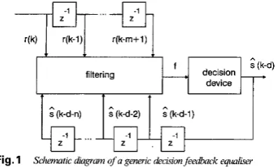
The generic DFE, depicted in Fig. 1, uses the information present in the channel observation vector

Space translation and linear separability

r ( k ) = [ r ( k ) . . . r ( k -

m

+

l)IT

(4)

and the past detected symbol vector

& ( k ) = [ . ? ( k - d - 1 ) . . . . ? ( k - d - n ) l T (5)

to produce an estimate J^(k -

d)

of s(k -

d).

The integers d,

m and n will be referred to as the decision delay, the feedforward and feedback orders, respectively. Without loss of generality, d = n, - 1, m = It, and n = nu - I wdl be used, as

t h ~ s choice of the DFE structure parameters is sufficient to guarantee the linear separability of the subsets of the channel states related to the different decisions (see lemma 1 in this Section).

filtering r(k)

I

r(k-l)l r(k-m+l)

1

;

(k-d)

decision device

i

t t 1 -

I

g(k-d-n)

I

g(k-d-2)

I

;(k-d-I)

I

Fig. 1 Schematic a’mgrm of a generk deckwn@e&k equalker

Applying the channel model, eqn. 1, to each element of the observation vector, eqn. 4, yields

where e(k) = [e@) ... e(k - m

+

1)]*, s(k) = [sfT(k)sbT(k)]* with

r ( k ) = F s ( k )

+

e ( k ) (6)

Sf(k) = [ s ( k ) . * . s ( k - d ) ] T

s b ( k ) = [ s ( k - d - l ) . ’ . s ( k - d - n ) l T (7)

and the rn x (d

+ 1 +

n) matrix F has the form

F = [ P I F 2 1 ( 8 )

with the m x (d

+

1) matrix Fl and m x n matrix F2 defined

...

by

1”

u1 una

1

and

r o

0

. . .

0

1

respectively. Under the assumption of correct decision feedback, that is, $&) = s&),

r ( k ) = F l s f ( k )

+

F2.%(k)

+

e ( k ) (11) Thus the decision feedback translates the original space v(k) into a new space ~’(k):

(12)

n

r ’ ( k ) = r ( k ) - F&(k)

348

This property was recogmsed in [6, 121. Previous research [13, 141 further pointed out that the elements of r’(k) can be computed recursively according to:

~ ’ ( k - i) = z - l r ’ ( k - i

+

1) - ~ , ~ ~ - i b ( k - d - 1)

i

= m - 1,

...,

2 , l r ’ ( k ) =

r ( k )

where z-l is interpreted as the unit delay operator.

t(k-I) r’(k-2) t(k-m+l)

filtering

decision device

s (k-d) S (k-d-I)

Fig. 2 Schenzatic diagram of trmlated deckwn feedback equaliser

Based on this interpretation of decision feedback, an alternative DFE structure is depicted in Fig. 2. Since a DFE is reduced to a transversal equaliser in the translated space, properties of the DFE can be studied more easily in the translated space. We have the following result of linear separability for the DFE.

Lemma

I:

Let the Nf = Md+’ sequences or states of sf(k) be

sfj, 1 s j s

Nf

The set of noiseless channel states in the translated space is defined by

A

R’ = { T ; = F i ~ f , j , 1

5 j

5

N f } (14) This set can be partitioned into A4 subsets conditioned on s(k - d) = si, 1 s i s M ,

e

{ T i E R’ls(k - d ) = Si} ₁

I

_i

I

_M

(15)

Idi), 1 s i s M , are linearly separable.

The proof of t h s lemma can be found in [14]. Lemma 1 shows that the mapping Fl: r’ = Fpf maps linearly separable sets in the sf space onto linearly separable sets in the v‘-space. This is in contrast to the case of an equaliser without decision feedback, where the mapping F: Y = Fs maps a large space s onto a smaller space Y. States which are linearly separable in the s-space will not necessanly be linearly separable in the u-space (see Appendix of [16]). Notice that we do not specify how r(k) and s^&) are combined here and, therefore, the results are valid for any DFE. It should be emphasised that, even though

R@,

1 s i s M , are linearly separable, the optimal decision boundary will generally be nonlinear (the Bayesian DFE

[q).

However, linear separability of the channel states related to the dfierent decisions is a highly desirable property to have because equalisation performance in this case is generally much better than that of the nonlinear separable case.

A simple example taken from [14] is used to illustrate the space translation property of decision feedback. Consider the two-tap channel

a = [UO u1IT = [0.5 1.OIT with 2-PAM symbols (16)

[image:2.613.95.294.219.338.2]

(3)

and the DFE with d = 1, m = 2 and n = 1. The set of 8-channel states in the original observation space u(k) is

depicted in Fig. 3. The decision feedback s(k - 2) corresponds to a space translation, the effect of whch is illustrated in Fig. 3. It can be seen that decision feedback effectively ‘merges’ channel states, and t h s simpMies the decision process. This space translation property was adopted in [17] to derive a concise version of the Bayesian DFE. Iltis [lS] has developed an importance sampling technique for evaluating the performance of the Bayesian equaliser, valid only for the case of linearly separable channel states. Lemma 1 shows that this importance sampling technique can readily be applied to evaluate the performance of the Bayesian DFE [Note 11.

2

-2

, ..

1 .

~(k-2) = 1

translated

0

~ ( k - 2 ) =-I

-2 -1 0 1 2

r(k) + r‘(k)

Fig.3

for channel Illustrutwn a = [0.5 1.01 of e p t with of U 2-PAM o!eckwnfeedbak s(k conrtellutwn - 2) on channel states

3 Linear-combiner DFE

The linear-combiner DFE is based on a linear filtering of

v(k) and i b ( k ) given by

f ( T ( k ) , g b ( k ) ) = WT,(k)

+

bT&,(k) (17)

where

w = [WO ’ * ’ W m - 1 I T

b = [bl

.

. . b,IT ₍₁₈₎

are the coefficients of the feedfonvard and feedback filters, respectively. Since the linear-combiner DFE is a special case of the generic DFE depicted in Fig. 1, by performing the translation eqn. 12, it is reduced to the equivalent linear equaliser:

The decision boundary of t h s equivalent equaliser consists of M - 1 parallel hyperplanes defined by: {U’: wTv’ =

2i

-

M } , 1 s i s M - 1. These hyperplanes can always be designed properly to separate the M subsets of the translated channel states R(n, 1 s i 5 M . One of the hyperplanes,

{Y’: wTr’ = 0}, passes through the origin of the r’(k)-space. Obviously, there must exist an MSER solution wopr for the structure in eqn. 19. The usual MMSE linear-combiner DFE, however, is not this MSER solution.

3.1

MMSE linear-combiner DFE

The Wiener solution for the linear-combiner DFE is well known (e.g. [Ill). Let fi and

8

be the MMSE solutions of

w and b. It can readily be shown that

f ’ ( T ’ ( k ) ) = W T T ’ ( k ) (19)

[:

I

=

[-&I

Note 1: CHEN, S.: ‘Importance sampling simulation for evaluating the lower-

bound BER of the Bayesian DFE‘, submitted to IEEE Trm. Comnnm., 1998 IEE Proc.-Commun., Vol. 146, No. 6, December 1999

with

y q =

Eap-+:tn:h(ll

O < q < r n - l

(24) and s(q) is the discrete Dirac delta function.

Since

fiTF2 =

-bT, we have

GT‘r(k)

+

L T S b ( k ) = h T ‘ r ’ ( k ) ₍₂₅₎ It merely confirms the space translation nature of decision feedback. Thus, when examining the MMSE linear-combiner DFE, we can simply study the feedforward part of the solution. In the asymptotic case of SNR

-

03, we have the following result for fi.

Lemma 2: In the noise-free case,

W Z

[

0 0 . . . 0

‘IT

a0 (26)

This result can be derived by setting 0,‘-+ 0 in eqn. 20, but an alternative proof is given in [14]. In the limit case of

SNR

-

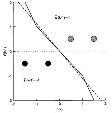
a, the hyperplanes of the MMSE solution are always orthogonal to the last axis of the v’(k)-space, which cannot be the optimal solution of eqn. 19 for any channel. Consider the example given in Fig. 3. The decision bound- ary of the Wiener solution for S N R -+ 60 is depicted in [image:3.616.316.511.481.678.2]

Fig. 4. The best possible h e a r decision boundary can easily be constructed for this example, which is very different from the MMSE solution. The true optimal Bayesian decision boundary in the asymptotic case is also illustrated in Fig. 4.

G(k-l)=l

s (k-I)=-1

‘I

A

\ \

-2 I I I I

-2 -1 0 1 2

r’ (k)

Fi . 4 Asymptotic decirion b o d r k s corresponding to h g e SNRfor chun- ne?a = [0,5 I.0IT with a 2-PAM constellation mddec&-wnfeedback

~ optimal Bayesian

_ _ _ best h e a r approximation

_ _ _ _ Wiener solution

(4)

When the noise is added, the hyperplanes of the MMSE linear decision boundary will rotate and are no longer orthogonal to the axis u'(k -

4.

Consider the example of Fig. 4 again. When SNR

-

0, the Wiener decision boundary will rotate towards the line with a slope -2 ($;idGI = 2), and there is no difference between the MMSE and MSER solutions. However, for meaningful SNRs, the difference between the MMSE decision boundary and the best linear boundary can be large. For example, given SNR = 15dB, the Wiener decision boundary is the line with a slope of -0.28, but the best linear decision boundary obtained by minimising the SER has a slope of -1.03. In general the MMSE solution is different from the MSER solution, and searching for the latter is worthwhile at least for certain channels.

3.2

MSER

linear-combiner

DFE

For the given channel model a = [a0 ... aiTc,-l]T and the noise variance

02,

the following lemma shows how to compute the SER of the linear-combiner DFE.

Lemma 3: Let 1 = MI2

+

1. The SER P d w ) of the linear- combiner DFE, with the weight vector w subject to the constraint

m-1

i=O is given by

where

00

1

Q ( x ) =

/

- exp

(-g)

dx

(30)

G

2

- v)Twl

llwll (31)

2

P3,1

+

P A 2 = -

llwll P3J =

and v can be any point in the hyperplane wTr' = 0. Since this hyperplane passes through the origin of the r'(k) space, we can always choose v = 0.

The derivation of this SER expression is given in the Appendix (Section 7.1). R(0 is the subset of channel states related to s(k -

d)

= sI = 1, and the number of states in R(0 is NfIM = M ' l u - l . Obviously, the MMSE solution does not

minimise

PAW).

Notice that the elements of w are not linearly independent. The constraint eqn. 27 is introduced to express the SER neatly in the form of eqn. 28, and it does not change the SER. It is worth pointing out that the low noise Wiener solution, eqn. 26, satisfies the constraint eqn. 27. The following algorithm can be employed to obtain the optimal weight vector wept for the MSER linear- combiner DFE.

Algorithm:

Step 1. Use a channel estimator to obtain a channel model and an estimate of the noise variance.

Step 2. Compute the subset of translated channel states R(0 and use the low noise Wiener solution, eqn. 26, as the initial value of w.

350

Step 3. Solve the optimisation problem,

m i n P E ( w ) , subject to wTareV = 1 ( 3 2 )

W to obtain a wept.

In the above algorithm, only step 1 involves channel observations. Once estimates of the channel model and noise variance are obtained, the optimisation eqn. 32 is car- ried out without involving any channel observation. This off-line optimisation problem can be solved, for example, using the augmented Lagrangian method [19], and an algorithm is given in the Appendix (Section 7.2). Computa- tional complexity of this MSER linear-combiner DFE is much more than that of the standard MMSE linear-combiner DFE. However, the performance gain can justify the increase in computation. Some of the channel states r20 are far away from the decision hyperplanes and contribute little to the SER. Computational requirements can be reduced by neglecting these states from the optimisation procedure with little performance degradation. For example, consider the case of Fig. 4. By just using the single state at (0.5, 0.5) in the optimisation, little performance degradation will occur, compared with using the full subset

R(*)

of the two states.

4 Numerical examples

Three examples were used to compare the MSER and MMSE solutions of the linear-combiner DFE. The optimal weight vector wept for the linear-combiner DFE was obtained using the algorithm described in the preceding Section. All the SERs were evaluated with detected sym-

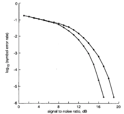
bols being fed back. The first example was the two-tap channel with 2-PAM symbols defined in eqn. 16. Fig. 5

compares the SERs of the MSER linear-combiner DFE with those of the MMSE linear-combiner DFE for a range of SNR conditions. For t h s example, the MSER linear- combiner DFE is superior and, at the SER of lo4, it has an SNR gain of -2dB over the Wiener solution.

-1 -

8

-2 -

L

-

2 -3

E 2

z

g -4

-

- -

-5

-

-6 I I I I I I I I I I

0 4 a 12 16 20

signal to noise ratio, dB Fi .5

bo

f

with detected symbols t%g,fed buck

MMSEIMSER: MMSWMSER linear-combiner DFEs

-0- MMSE

-f- MSER

P e f o m c e corn misonfor c h w l a = [ O S I.OIT (Md2-PAMsyn-

The second example was a 5-tap channel with the 2- PAM constellation:

a = [0.227 0.466 0.688 0.466 0.227IT

with 2-PAM symbols ( 3 3 )

[image:4.612.331.540.423.615.2]

(5)

The structure of the DFE was chosen to be d =

4,

rn = 5

and n = 4. The SERs of the MSER and MMSE linear- combiner DFEs with detected symbols being fed back are plotted in Fig. 6, where it can be seen that the performance of the MSER linear-combiner DFE is sigmfkantly better than that of the MMSE solution. At the SER of lo4, the MSER solution has an SNR gain of -1 dB over the MMSE solution.

-1

h

2 -2

E

e

b 0 -3 n

L

-

5

1

z

8 -4

-

-5

.

’

-6 I I

8 10 12 14 16 18 20 22

signal to noise ratio, dB

Fig.6

O.227lT mud 2-PAM syinhof

\th

kected syinhols beingfed buck

MMSWMSER: MMSEiMSER linear-combiner DFEs -0- MMSE

-+-

MSER

Perjormunce coin atison or clumnel a = 10.227 0.466 0.658 0.466

The third example was a 3-tap channel with the 4-PAM constellation:

a = [0.3482 0.8704 0.3482IT

with 4-PAM symbols (34)

The structural parameters of the DFE were set to d = 2, rn

= 3 and n = 2. The SERs of the MSER and MMSE linear- combiner DFEs with detected symbols being fed back are depicted in Fig. 7. Again, the MSER solution is superior and has an SNR gain over 1dB at the SER of l p , compared with the MMSE solution.

-

16 18 20 22 24 26 28

2 . 7 Peflomuuiw cornpurison jbr c l m l a = (0.3482 0.8704 0.3482IT signal to noise ratio, dB

C P A M symbols with rktecied synrbols bemg fed buck

MMSEJMSER: MMSUMSER linear-combiner DFEs -0- MMSE

-+- MSER

IEE Proc.-Commun., Vol. 146, No. 6, Deceniher 1999

5 Conclusions

We have derived an SER expression of the linear-combiner DFE for the general M-PAM constellation. This is made possible by utilising a geometric translation property of the decision feedback in the DFE structure. Basically, the decision feedback performs a space translation that maps the DFE onto an equivalent transversal equaliser in the translated observation space and, furthermore, the subsets of translated channel states corresponding to the different decisions are always linearly separable. In particular, viewed from the translated observation space, the linear- combiner DFE is reduced to a linear equaliser and, moreo- ver, the hyperplanes of the Wiener solution under very low noise conditions are orthogonal to the last axis of the translated space. This shows that the MMSE solution does not achieve the full performance potential of the linear-combiner DFE structure. An algorithm is proposed to obtain the MSER solution by minimising the SER criterion. Numerical examples have been included to illustrate the better performance of the MSER linear-combiner DFE over the MMSE solution for certain channels. A drawback of this MSER solution is a significant increase in computational complexity compared with the Wiener solution.

The algorithm presented in this paper for obtaining the MSER solution is an off-line algorithm. For communication links, practical application of this algorithm is limited to the initial set-up of the DFE. This MSER linear-combiner DFE in its present form is more suited for data storage systems, as in many commercial disk drives the equalisers are trained at the factory floor and then are ‘frozen’ before shipping. Ongoing research will investigate how to implement this MSER linear-combiner DFE adaptively, so that it can be applied to fast time-varying channels.

6

1

2

3

4

5

6

7

8

9

References

QURESHI, S.U.H.: ‘Adaptive equalization’, Proc. IEEE, 1985, 73,

(9), pp. 1349-1387

PROAKIS, J.G.: ‘Digital commnnications’ (McGraw-Hill, New York, 1995, 3rd edn.)

MOON, J.: ‘The role of SP in data-storage systems’, IEEE Signul Process. Mug., 1998, 15, (4), pp. 54-72

PROAKIS, J.G.: ‘Equalization techniques for high-density magnetic recording’, IEEE Signul Process. Mag., 1998, 15, (4), pp. 72-82

SIU, S., GIBSON, G.J., and COWAN, C.F.N.: ‘Decision feedback equalisation using neural network structures and performance compar- ison with the standard architecture’, IEE Proc. I, Cotnmzm. Speech Vis., 1990, 137, (4), pp. 221-225

WILLIAMSON, D., KENNEDY, R.A., and PULFORD, G.W.: Block decision feedback equalization’, IEEE Truns. Comtmm, 1992, 40, (2), pp. 255-264

CHEN, S., MULGREW, B., and McLAUGHLN, S.: ‘Adaptive Bayesian equaliser with decision feedback’, IEEE Truns. Signal Proc- ess., 1993, 41, (9), pp. 2918-2927

CHEN, S., McLAUGHLIN, S., and MULGREW, B.: ‘Complex-valued radial basis function network, Part 11: application to digital communications channel equalisation’, EURASIP Signul Procem. J., 1994,

36, pp. 175-188

CHEN, S., McLAUGHLIN, S., MULGREW, B., and GRANT, P.M.: ‘Adaptive Bayesian decision feedback equaliser for dispersive mobile radio channels’, IEEE Truns. Conlmun., 1995, 43, (5), pp. 1937-1 946

I O CHA, I., and KASSAM, S.A.: ‘Channel equalization using adaptive complex radial basis function networks’, IEEE J. Se/. Areus Commun.,

1995, 13, (l), pp. 122-131

11 CIOFFI, J.M., DUDEVOIR, G.P., EYUBOGLU, M.V., and FOR- NEY, G.D.: ‘MMSE decision-feedback equalizers and coding - part

1: equalization results’, IEEE Trcins. Coniinun., 1995, 43, (lo), pp. 2582-2594

12 CLARK, A.P., LEE, L.H., and MARSHALL, R.S.: ‘Developments of the conventional non-linear equaliser’, IEE Proc F, Commun. Rudur Signul Process., 1982, 129, (2), pp. 85-94

13 CHEN, S . , CHNG, E.S., MULGREW, B., and GIBSON, G.: ‘Mini- mum-BER linear-combiner D F E . Proceedings of ICC‘96, Dallas, TX,

1996, Vol. 2, pp. 1173-1177

(6)

14 CHEN, S., MULGREW, B., CHNG, E.S., and GIBSON, G.: 'Space translation properties and the minimum-BER linearcombiner D F E ,

IEE Proc. Commun.. 1998, 145, (5), pp. 316-322

15 YEH, C.C., and BARRY, J.R.: 'Approximate minimum bit-error rate equalization for pulse-amplitude and quadrature-amplitude modulation'. Proceedings of lCC'98, Atlanta, USA, 1998, Vol. 1, pp. 16-20 16 GIBSON, G.J., SIU, S., and COWAN, C.F.N.: 'The application of

nonlinear structures to the reconstruction of binary signals', IEEE Trans. Signal Process., 1991, 39, (8), pp. 1877-1884

17 CHEN, S., McLAUGHLIN, S., MULGREW, B., and GRANT,

P.M.: 'Bayesian decision feedback equaliser for overcoming co-channel interference', IEE Proc. Commun., 1996, 143, (4), pp. 219-225 18 ILTIS, R.A.: 'A randomized bias technique for the importance sam-

pling simulation of Bayesian equalizers', IEEE Tram Commun., 1995, 43, (2/3/4), pp. 1107-1 115

19 BAZARAA, M.S., SHERALI, H.D., and S H E W , C.M.: 'Nonlin- ear programming: Theory and algorithms (John Wdey, New York, 1993)

7 Appendixes

7.

I

Derivation of

SER

expression

Consider the hear-combiner DFE, eqn. 19. The M - 1 hyperplanes {U': wTv' = 2i - M } , 1 s i s M - 1, partition the m-dimensional v'-space into M regions:

z(2)

i2

{r' :

8(5

- d ) = Si} 1

5

i

5

M

( 3 5 )

The SER

of

the linear-combiner DFE is a function of w and can be expressed as

M

3 r ' 3 Z ( * )

where p,'(v'lv,(n) is the probability density function of

v'(k)

conditional on the received channel state being v-3, f i ( l 1 is

the a priori probability of P,@ and 3 denotes 'not in'. Taking into account the fact of symmetry and equiproba- ble states, eqn. 36 is reduced to

t=1 r ( t ) E R ( % )

(36)

where

p,

(

r ( 4

)

n

-

/

prl

( T ' I T ~ ~ ) )

dr' ₍₃₈₎

r ' 3 2 ( ' )

is the conditional error probability when the received channel state is vj'" E R(Q.

I

'0'

Fig. 8 Computation of conditionul error probability

Consider the subset of channel states R(o, where 1 = MI2

+

1. RO is separated from other subsets by two hyperplanes wTv' = 0 and wTv' = 2. Referring to Fig. 8, an orthogonal transformation x =

Lv'

can be constructed whch rotates the bases so that one of the transformed bases, say xo, is parallel to w, the normal of the decision hyperplanes. Since

352

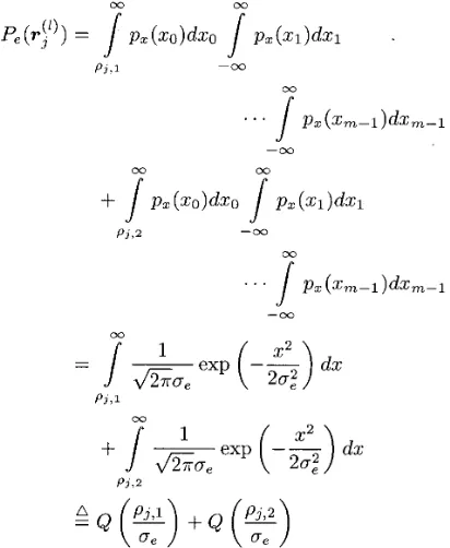
LLT = I and the whte noise e(k) has a Gaussian distribu- tion, the conditional error probability Pe(r)o) can be computed as

00 00

P,(r:l))

=

/

pz(zo)dzo

/

P z ( z l ) d z l

+

/

pz(z0)dzo

/

P z ( z l ) d z l

P3,I -00

. . .

7

pz ( z m - 1 )dxm-l -00

00 03

P 3 > 2 -00

00

-

/

&exp

(-z)

dx

20:

P 3 > 1

00

1 exp

(-5)

2a,2

dx

P 3 . 2

Q

(

F)

+

Q

(

F)

(39) where pj,l and pj,2 are the Euclidean distances between

vjo

and the hyperplanes wTv' = 0 and wTv' = 2, respectively. It can easily be seen that

I(?-?)

- Z))TwI (40) 2

llwll Pj,l

+

P j , 2 = -

l l 4 l

P j , l =

and v can be any point in the hyperplane wTr' = 0.

R('+') is a translation of R(Q:

From eqns. 9, 14 and 15, it is obvious that the subset

R(Z+l) =

di)

+

( s z + 1 - Si)[U,,-l

.

f * U l U O ] T

= R(i)

+

2arev (41) where urev = [ana-l

...

alaolT. Notice that the elements of w

are linearly dependent. Specfiically, if we impose the following constraint:

m - 1

i=O

the (i

+

1)th hyperplane is the translation of the ith hyperplane by the amount 2urev. As illustrated in Fig. 8, it becomes evident that

and

(44)

Thus the SER of the linear-combiner DFE is given by

PE

('UI)

(45)

[image:6.613.335.541.80.331.2]

(7)

The feedforward weights of the equaliser are subject to the constraint eqn. 42.

7.2 Algorithm for solving the optimisation problem

Define the augmented Lagrangian function

~ E ( w ? A ? = p E ( w )

+

A ( W T a r e u - 1)

+

CL(wTa,ev - (46)

The following algorithm [19] can be used to solve the optimisation problem, eqn. 32.

Initialisation. Choose A, p > 0 and w(0); give a termination scalar E > 0; set t = 1.

Loop. Solve the unconstrained optimisation problem

w(t) = min W PE(w,

A,

p ) (47)

If ~wT(t)ur,, - 11 < E : goto stop;

goto Loop;

2p(Wqt)u,,, - l), t = t

+

1, goto Loop.

Else if $vT(t)ure,, - 11 > 0.251wT(t - I)ure, - 11 : p = 1O.Op,

Else if IwT(t)u,,,, - 11 I 0.251wT(t ~ l)ure, - 11 :

A

= A

+

Stop. w(t) is the solution.

The unconstrained optimisation problem, eqn. 47, is solved using a simplified conjugate gradient method. For convenience, drop A and p in

BE,

and define the gradient vector

= VPE(w)+Aa,e,+2p(wTa,e, - 1 ) a r e v

(48)

Initialisation. Choose a small step size a > 0 and a termination scalar

p

> 0; given w(1) and d(1) = -VPE(w(1)); s e t j = 1.

Loop. If IlVPE(w(j)>ll <

p

: goto stop.

WO'

+

1) = W O ]

+

CY&),

@ =

ll~~~~(i+1))112~11~~Ei~03)112

d(j

+

1) = @@j] - Vpdwg'

+

1 ) ) , j = J

+

I , goto Loop.

The derivatives of P d w ) with respect to wj, 0 5 i 5 m ~ 1,

Stop. wfj] is the solution.

are

a p E ('U))

d W i

(49)

with

(50)

and

(51) where I = MI2

+

1, s a ( . ) is the signum function, v, and r,;,(o are the ith elements of v and r>o, respectively, v is any point in the hyperplane wTiJ = 0, and pJ,l and pJ,2 are defined in

eqn. 31.