A High Order Accurate MultiGrid Pressure Correction Algorithm for Incompressible Navier-Stokes Equations

(1)

A High Order Accurate MultiGrid Pressure

Correction Algorithm for Incompressible

Navier-Stokes Equations

V. Mandikas, E. Mathioudakis, E. Papadopoulou and N. Kampanis

Abstract—A fourth-order accurate finite-difference compact numerical scheme coupled with a geometric MultiGrid tech-nique is introduced for an efficient incompressible Navier-Stokes solver on staggered meshes. Incompressibility condition is enforced iteratively by solving a Poisson-type equation performing global pressure correction. Its application is the most computationally demanding part of the algorithm and in order to save computation cost a MultiGrid technique is applied to accelerate the iterative procedure of pressure updates at each time step. Appropriate boundary closure formulas are developed in case of the cell-centered approximations which implement the boundary conditions. Geometric MultiGrid techniques are not straightforward in this case, because the coarse grids do not constitute part of the fine grids. Suitable classical restriction and extension operators are modified for the efficient application of MultiGrid procedure. The performance investigation of realistic applications on non-high performance computing environments resulted that the MultiGrid technique can accelerate significantly the numerical solution process, holding at the same time the high accuracy of the numerical method even for high Reynolds numbers.

Index Terms—Incompressible Navier-Stokes equations, Com-pact Finite Differences schemes, staggered grids, Geometric MultiGrid techniques.

I. INTRODUCTION

I

N many practical applications, high resolution and fast solvers for incompressible Navier-Stokes equations are needed, such as in fine structured engineering on flows with high Reynolds number, where detailed flowfield in-formation is required. The incompressibility constraint can be applied through various procedures, [1], [2]. In [3] it was proposed an iteratively procedure at each time step, until velocities computed satisfy the continuity equation to machine precision. A traditional approach is that of cell-by-cell pressure corrections applied iteratively until velocity practically satisfies the continuity equation, [4]. Numerical experiments showed that by increasing the Reynolds number, the number of iterations required by the local pressure cor-rection method per time increase fast, making the associated computational cost intolerable. An alternative approach is

Manuscript received February 20, 2013; revised April 16, 2013. Corresponding author’s e-mail: [email protected].

This research was supported in part by the special grant GZF030/2009-10 for Scholar’s Association of Alexander S. Onassis Public Benefit Founda-tion.

V. Mandikas, E. Mathioudakis and E. Papadopoulou are with the Department of Sciences, Division of Mathematics, Technical University of Crete, University Campus, 73132 Chania, Crete, Greece email: [email protected], [email protected] and [email protected]

N. Kampanis is with the Institute of Applied and Computational Mathe-matics, Foundation for Research and Technology - Hellas, 70013 Heraklion, Greece email:[email protected]

to solve the Poisson equation satisfied by the pressure cor-rections which are obtained from the momentum equations, and obtain the pressure field distribution in terms of the velocities. Pressure correction computation using the Poisson equation is employed in several effective methods proposed for the numerical solution of the incompressible Navier-Stokes equations, [5], [6], [7]. An important observation for the pressure correction computation, using the Poisson equation is that, for high Reynolds number, the number of iterations required for incompressibility remains lower, [8], than that for the cell-by-cell pressure correction procedure. The application of the Poisson-type pressure correction pro-cedure produces a large and sparse linear system of algebraic equations, suggesting the use of iterative solvers to save computational cost. Execution time for the solution of the linear system remains a forbidding factor for realistic appli-cations on non-high performance computing environments. But significant convergence acceleration can achieved with the incorporation of geometric MultiGrid techniques into the iterative solver [9], [10], [11], [12], [13], [14].

We develop an algorithm based on a high order accurate finite difference method, more specifically on the fourth-order compact numerical scheme, which subsequently is applied to a cell-centered grid and the resulting algorithm is implemented for the pressure correction procedure in two di-mensions as an extension of the numerical method introduced in [8]. In the proposed scheme a major innovation amounts to the treatment of realistic boundary conditions, since we focus to actual applications in fluid mechanics. Boundary closure formulas, for Dirichlet boundary conditions valid on the physical boundary, are derived and presented here in. In order to accelerate the pressure correction procedure a MultiGrid technique is applied and appropriate intergrid transfer operators with special treatments for boundary clo-sures are constructed for this purpose. This paper is organized as follows: In Section 2, the overall numerical method based on a fourth order cell-centered compact difference scheme, for the pressure correction based on the Poisson-type equation is described. In Section 3, the MultiGrid technique is considered for accelerating the update pressure-correction procedure. Finally, Sections 4 and 5, present the numerical results and the performance investigation of the algorithm implementation and the conclusions respectively.

II. THE INCOMPRESSIBLENAVIER-STOKES SOLVER

(2)

The incompressible Navier-Stokes equations in Cartesian (x, y)coordinates can be expressed as:

∂u

∂x +

∂v

∂y = 0, (1)

∂u

∂t +

∂F

∂x +

∂G

∂y =−∇p+

1

Re

∂F_v

∂x +

∂Gv

∂y

,(2)

whereu= [u, v,]T andp are the velocity vector and pres-sure, respectively, and Re=U L/ν is the Reynolds number based on a characteristic velocity U and a characteristic lengthL. Furthermore,FandGare the inviscid flux vectors, while Fv andGv are the viscous fluxes given by

F= [u2, uv]T, G= [vu, v2]T,

Fv=

h∂u

∂x,

∂v ∂x

iT

, Gv=

h∂u

∂y,

∂v ∂y

iT

.

Using appropriate finite compact centered schemes on stag-gered grids, a fourth-order accuracy in space was obtained in [8]. The overall fourth order accurate numerical method, is not able to model properly incompressible flows at high Reynolds numbers, due to the increase of the computational cost for incompressibility condition. This limitation can be overcame by using MultiGrid techniques in order to accel-erate the numerical solution of the Poisson-type equation discretized by high order finite difference methods. Specif-ically, a fourth order compact scheme is used to discretize the Poisson-type equation. The use of compact descritizations additionally serves the treatment of boundary conditions with one layer of fictitious cells in outward along the boundary. Unlike compact methods, classical finite differences require wider fictitious layer making the use in curvilinear domains inappropriate. The explicit Runge-Kutta [15], time-marching scheme fourth-order accuracy is employed for the time semidiscretization. This amounts to the time stepping through the following intermediate steps:

Un,1=Un, Pn,1=Pn (3)

Un,2=Un+∆t 2 R

n,1_, ₍₄₎

Un,3=Un+∆t 2 R

n,2_, ₍₅₎

Un,4=Un+ ∆tRn,3, (6)

Un+1=Un+∆t 6 (R

n,1_{+ 2}_Rn,2_{+ 2}_Rn,3₊_Rn,4₎

(7)

withtn₌_n_∆_t_,_tn,1₌_tn_,_tn,2₌_tn,3₌_tn_{+ ∆}_t/₂_,_tn,4₌

tn_{+ ∆}_t_{, and} _Rn,` ₌ _R₍_Un,`_{, P}n,`_;_tn,`₎_{, for} _` _{= 2}_,₃_,₄_, whereR(U,P;t) is the right-hand side of (2).

The quantities Pn,`_, _` _{= 2}_,₃_,₄ _and_Pn+1_{, appearing in}

(3)-(7), are determined by enforcing the incompressibility on the velocity vectors Un,`_, _` _{= 2}_,₃_,₄ _and _Un+1_.

In-compressibility is enforced on the velocity vectors Un,`,

` = 2,3,4, and Un+1 by the pressure update procedures described below.

The velocities vectors Un+1(as well as the intermediate stages Un,`, ` = 2,3,4) do not (necessarily) satisfy the incompressibility condition (1). The computed velocity field at each time step (and the intermediate stages) should be corrected to satisfy (1) usually iteratively through suitable

-6

0

Y

Ly

X Lx

r r r r

b b b b b b

b b

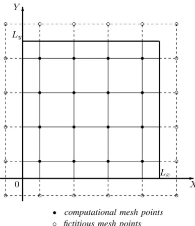
[image:2.595.338.532.52.276.2]

r computational mesh points b fictitious mesh points

Fig. 1. The pressure correction computational grid.

pressure updates. Pressure updates at each time step may be corrected for all cells simultaneously obtained by computing pressures corrections for all cells locally computed in a cell by cell advancing procedure. This however results in a low order, lowly convergence procedure with poor effectiveness especially at higher Reynolds numbers where flow patterns are significantly complex. As a consequence, the Poisson-type equation must be solved several times making the application of a MultiGrid technique necessary. The spatial derivatives appearing in the continuity equation during the pressure update procedures, are computed using fourth-order accurate compact formulas.

As an alternative, [8], the following Poisson-type equa-tion for the pressure correcequa-tion ∆p defined globally on Ω ≡ [0, Lx]×[0, Ly], and valid at the cell centers Mij,

i= 1, ..., Nx,j= 1, ...Ny:

_∂2_(∆_p₎

∂x2

ij +

_∂2_(∆_p₎

∂y2

ij

=fij (8)

withfij =f(Mij) = _a 1

`,`−1∆t(∇ ·u

n,` old).

The boundary conditions for the pressure correction ∆p

and pressure are associated. For Dirichlet boundary condi-tions,pis constant, therefore∆p= 0. For Neumann bound-ary conditions, ∂p/∂n = 0, that implies ∂(∆p)/∂n = 0, with n the outward normal on the boundary. The solution ∆p(x, y) and the right-hand side function f(x, y) are as-sumed to be sufficiently smooth and have the required con-tinuous partial derivatives. The fourth order finite difference compact numerical method is seeking for an approximation of pressure corrections solution at the center node of each computational cell of Ω, since our computational grid is a staggered one. There are n= NxNy centered mesh points (xi−1/2, yi−1/2),i= 0,1, . . . , Nx+ 1,j= 0,1, . . . , Ny+ 1 insideΩ, and they can be assumed as grid points of a new shifted computational grid (xi, yi), i = 0,1, . . . , Nx + 1,

(3)

and j = 0, Ny + 1 are the fictitious mesh points, Fig. 2. The fourth order compact approximation scheme, which is mathematically equivalent to [16], can be expressed as

d(∆pi+1,j+1+ ∆pi+1,j−1+ ∆pi−1,j+1+ ∆pi−1,j−1)

+c(∆pi+1,j+ ∆pi−1,j) +b(∆pi,j+1+ ∆pi,j−1)

−a∆pi,j

= ∆x

2

2 (8fi,j+fi+1,j+fi−1,j+fi,j+1+fi,j−1), (9)

witha= 10(1 +γ2), b= 5−γ2, c= 5γ2−1, d= (1 +γ2₎_/₂ _and_γ_{= ∆}_x/_∆_y _{the mesh ratio.}

Since the new shifted computational grid coincides with the center nodes of the staggered grid, the incorporation of the actual boundary conditions is not straightforward. To this end, the following treatment procedure of boundary conditions is introduced by the authors. Following [17], the interpolation formula

φi+1

2 +αφi+ 3

2 =aφi+bφi+1+cφi+2+dφi+3, (10)

withα=f ree, a= ₁₆5 − a

16,b= 15 16 +

9a

16,c=− 5 16 +

9a

16

andd= ₁₆1 − a

16, is used. This procedure relates values on

the original structure grid (i+ 1, i+ 2, i+ 3) with values on the new shifted grid (i+ 1/2, i+ 3/2), and is used for the implementation of Dirichlet boundary conditions.

Accordingly, [17],

φ0_i₊1 2+αφ

0 i+3

2 =aφi+bφi+1+cφi+2+dφi+3+eφi+4, (11)

with α = f ree, a = −22

24 +

a

24, b = 17 24 −

9a

8, c = 3 8 + 9a

8, d = − 5 24 −

a

24 and e = 1

24, is used for the case of

Neumann boundary conditions. The above formulas (10) and (11) simplify to

φi=

16

5 φi+12 −3φi+1+φi+2−

1

5φi+3 (12)

φi=−

12 11φ

0 i+1

2 +

17 22φi+1+

9 22φi+2−

5 22φi+3+

1 22φi+4

(13) for α= 0.

The zebra coloring scheme for numbering unknowns and equations is adopted for the linear system in (9) , which guarantees a desirable potential high degree of parallelism and scalability [18], [19], [20]. This type of coloring scheme produces the coefficient matrixA∈_Rn×n_{of the fourth order} cell-centered compact difference scheme in the following block form

A =



               

A1A2 O . . . O O O A3A4 O . . . O O O

O A5 O . . . O O O A6A6 O . . . O O O

O O A5. . . O O O O A6A6. . . O O O

. . .

. . . . ..

. . .

. . . . ..

. . .

O O O . . . A5 O O O O O . . . A6 O O

O O O . . . O A5 O O O O . . . A6A6 O

O O O . . . O O A5 O O O . . . O A6A6

A6A6 O . . . O O O A5 O O . . . O O O

O A6A6. . . O O O O A5 O . . . O O O

O O A6. . . O O O O O A5. . . O O O

. . .

. . . . ..

. . .

. . . . ..

. . .

O O O . . . A6A6 O O O O . . . A5 O O

O O O . . . O A6A6 O O O . . . O A5 O

O O O . . . O A4A3 O O O . . . O A2A1



               

,

(14)

-6

0 X

Nx

d d d d

s s s s s s s s s s s s s s s s s s s s s s s s s s s s s s s s s s s s s s s s s s s s s s s s s s s s s s s s s s s s s s s s

d_−→ _vH

i,j , s−→ vi,jh

Fig. 2. Fine and Coarse grid discretization and residual nodes.

with the order of submatricesAi for i= 1, . . . ,4 beenNx. Robin or mixed boundary conditions can be treated similarly, eliminating the fictitious nodes combining the approximation formulas (12) and (13).

III. MULTIGRID SOLVER FOR PRESSURE CORRECTION

(4)

v₂h_i,₂_j =₁₆1(9vH_i,j+ 3v_iH₊₁_,j+ 3v_i,jH₊₁+vH_i₊₁_,j₊₁)

vh

2i+1,2j =

1 16(3v

H

i,j+ 9vHi+1,j+vi,jH+1+ 3vHi+1,j+1)

v₂h_i,₂_j₊₁ =₁₆1(3vH_i,j+v_iH₊₁_,j+ 9vH_i,j₊₁+ 3vH_i₊₁_,j₊₁)

vh

2i+1,2j+1= 1 16(v

H

i,j+ 3viH+1,j+ 3vi,jH+1+ 9vHi+1,j+1)

(15)

for i = 1, ...,Nx

2 −1 and j = 1, ...,

Ny

2 −1 and is called

bilinear interpolation (IH

h ) operator. For all components of

vh _{corresponding to points close to the boundary, fictitious} coarse points values are involved lying outside the boundary area. These values can be eliminated using the boundary con-ditions. For the case of Dirichlet with zero valued function and Neumann boundary condition cases the components of fine vector close to they= 0 boundary are giver by

vh

2i+1,1= 1 8(v

H

i,1+ 3vHi+1,1), vh2i,1= 1 8(3v

H

i,1+viH+1,1)

(16) and

vh

2i+1,1= 1 4(v

H

i,1+ 3vHi+1,1), vh2i,1= 1 4(3v

H

i,1+viH+1,1)

(17) respectively, for 1 ≤i≤ Nx

2 −1. Other points close to the

boundary are similarly treated.

Choosing as a restriction operatorIH

h the one that satisfies the relation

IHh =

1 4I

H

h ,

then in stencil notation it is defined as

I_Hh = 1

64 

  

1 3 3 1

3 9 9 3

1 3 3 1



  

. (18)

In the MultiGrid algorithm the V-cycle scheme is chosen which can decrypted with the following compact recursive algorithm

V-cycle algorithm

∆pm_k+1=mgvcycle(k,∆pmk, Ak, fk, v1, v2) Presmoothing:

∆pmk =smoothv1(∆pmk, Ak, fk) Restriction:

fm

k−1=Ikk−1(fk−Ak∆pkm) Recursion:

ifk= 1use a fast iterative solver forAk−1∆pmk−1=f m k−1 ifk >1 ∆pmk−1=mgvcycle(k−1,0, Ak−1, fkm−1, v1, v2) Interpolation:

∆pm

k = ∆pmk +Ik −1 k ∆p

m k−1 Postsmoothing:

∆pm_k+1=smoothv2_(∆_pm k, Ak, fk)

The above algorithm calculates the new approximation ∆pm_k+1 at iteration stepm+ 1of the linear system solution ∆pk from the previous one∆pmk . The subscriptk indicates the grid level with k = 1 corresponding to finest grid. In the description of the V-cycle algorithm, performing v

smoothing steps with an iterative solver e.g Gauss-Seidel [21], [11], [14], [12], applied to any discrete problem of the formAk∆pk=fkwith initial approximation∆pkis denoted by thesmoothv _{procedure. Usually the number of pre- and} postsmoothing iterations in the descent and ascent phase of V-cycle are both equal to2. For the multigrid levels of V-cycle, the matricesAk at the coarse levels are determined by discretizing the Poisson-type equation on the corresponding coarse grid. The smoother Gauss-Seidel iterative solver is based on the following slitting of the coefficient matrix

A=DA−LA−UA where

DA :=

                

A1A2 O . . . O O O O O O . . . O O O

O A5 O . . . O O O O O O . . . O O O

O O A5. . . O O O O O O . . . O O O

. . . . . . . . . . .. . . . . . . . . . . . . . . . . . . . .. . . . . . . . . .

O O O . . . A5 O O O O O . . . O O O

O O O . . . O A5 O O O O . . . O O O

O O O . . . O O A5 O O O . . . O O O

O O O . . . O O O A5 O O . . . O O O

O O O . . . O O O O A5 O . . . O O O

O O O . . . O O O O O A5. . . O O O

. . . . . . . . . . .. . . . . . . . . . . . . . . . . . . . .. . . . . . . . . .

O O O . . . O O O O O O . . . A5 O O

O O O . . . O O O O O O . . . O A5 O

O O O . . . O O O O O O . . . O A2A1

                 ,

−LA :=                 

O O O . . . O O O O O O . . . O O O O O O . . . O O O O O O . . . O O O O O O . . . O O O O O O . . . O O O

. . . . . . . . . . .. . . . . . . . . . . . . . . . . . . . .. . . . . . . . . .

O O O . . . O O O O O O . . . O O O O O O . . . O O O O O O . . . O O O O O O . . . O O O O O O . . . O O O A6A6 O . . . O O O O O O . . . O O O

O A6A6. . . O O O O O O . . . O O O

O O A6. . . O O O O O O . . . O O O

. . . . . . . . . . .. . . . . . . . . . . . . . . . . . . . .. . . . . . . . . .

O O O . . . A6A6 O O O O . . . O O O

O O O . . . O A6A6O O O . . . O O O

O O O . . . O A4A3O O O . . . O O O

                 and

−UA :=                 

O O O . . . O O O A3A4 O . . . O O O

O O O . . . O O O A6A6 O . . . O O O

O O O . . . O O O O A6A6. . . O O O

. . . . . . . . . . .. . . . . . . . . . . . . . . . . . . . .. . . . . . . . . .

O O O . . . O O O O O O . . . A6 O O

O O O . . . O O O O O O . . . A6A6 O

O O O . . . O O O O O O . . . O A6A6

. . . . . . . . . . .. . . . . . . . . . . . . . . . . . . . .. . . . . . . . . .

                 .

IV. NUMERICALEXPERIMENTS

(5)

Fig. 3. Spatial accuracy against the analytical solution for the Taylor Vortex problem with Re=100, 1000 and 10000.

Problem 1:Taylor vortex.

In order to confirm the spatial accuracy of the algo-rithm implementation for every choice of Reynolds number, we solved the Taylor vortex problem [22] on the domain [−1,1]×[−1,1] with Dirichlet boundary conditions. The initial condition is based on the exact solution:

u= (−cos(πx) sin(πy)i+ sin(πx) cos(πy)j) exp

₋₂_π2_t

Re

p=−1

4(cos(2πx) + cos(2πy)) exp

₋₂_π2_t

Re

(19)

where Re=1/v been the Reynolds number and considered as Re ∈ {10,102_,₁₀3_}_{. The time step size} _∆_t _{= 10}−5

was chosen to satisfy the CFL condition and to ensure that the dominant error was the spatial error. The results are summarized in Fig. 3. The convergence rate of L2 _norm

for velocity and pressure error evaluated at the final time measurement T=5, is 4 for all choices of Re.

Problem 2:Driven cavity flow.

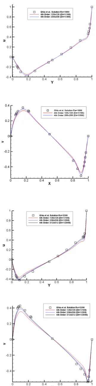
We also considered the steady-state driven cavity flow problem with well-defined boundary conditions on the unit square. Numerical solutions were obtained at different Reynolds numbers and compared with the computations of

[image:5.595.82.237.80.386.2] [image:5.595.303.557.364.415.2]

Ref. [23]. Fig. 4 presents the agreement with the solution approximation of Ghia et al forRe= 1000andRe= 3200. On a 256×256 grid or finer for Re = 1000 the solution can be approximated sufficiently. Nonetheless, increasing the Reynolds numbers to 3200 a finer grid must be applied as shown on the two bottom plots. Tables 1 and 2 present the total number of Poisson-type equations required to be solved in all stages of Runge-Kutta time marching procedure, until time reaches the end in order to enforce incompressibility condition iteratively. Additionally, the average cpu time in seconds for approximating the solution of every Poisson-type equation is shown. These time measurements are also presented for the corresponding method proposed in [8] . As shown, our New method’s algorithm has reduced sig-nificantly the number of Poisson-type equations required to be solved in all cases. An important outcome of this performance investigation is that every Poisson-equation is solved faster as the Reynolds number increases for the new algorithm. This is due to the application of the fourth order compact scheme with the multigrid technique, because high Reynolds numbers produce more oscillatory solutions corresponding to more oscillatory errors. It is well-known that a multigrid technique quickly eliminates the oscillatory error components.

Table 1

Total number of Poisson-type equations forRe= 1000and T=35.

grid size Method in [8] New Method

No. Poisson Time/Poisson No. Poisson Time/Poisson

64 224710 0.015 121705 0.006

128 613226 0.147 131124 0.025

[image:5.595.302.557.459.517.2]

256 1756002 1.513 219869 0.105

Table 2

Total number of Poisson-type equations forRe= 3200and T=75.

grid size _{No. Poisson}Method in [8]_Time/Poisson _{No. Poisson}New Method_Time/Poisson

64 300150 0.015 155817 0.006

128 709023 0.149 265375 0.015

256 1600310 1.515 430163 0.062

512 - - 996746 0.318

V. CONCLUSION

(6)

[image:6.595.70.232.86.732.2]

Fig. 4. Comparison of the horizontal and vertical velocity compo-nents computed with the reference solution by Ghia et al.

REFERENCES

[1] A. Chorin, “A numerical method for solving incompressible, viscous flow problems,”J. Comp. Physics, vol. 2(1), pp. 12–26, 1967. [2] C. Merkle and M. Athavale, “Time-accurate unsteady incompressible

flow algorithms based on artificial compressibility,”AIAA Paper, pp. 87–1137, 1987.

[3] J. D. Anderson,Computational Fluid Dynamics. New York: Mc-GrawHill, 1995.

[4] C. Hirt, B. Nichols, and N. Romero, “SOLA: a numerical solution algorithm for transient fluid flows,” inLos Alamos Report LA-5852, 1975.

[5] A. Chorin, “Numerical solution of the Navier-Stokes equations,”Math. Comput., vol. 22, pp. 745–762, 1968.

[6] R. Issa, “Solution of the implicitly discretised fluid flow equations by operator-splitting,”J. Comp. Physics, vol. 65, pp. 40–65, 1985. [7] S. Patankar,Numerical Heat Transfer and Fluid Flow. Washington,

DC: Hemisphere Publishing Co., 1980.

[8] N. Kampanis and J. Ekaterinaris, “A staggered grid, high-order accu-rate method for the incompressible Navier-Stokes equations,”J. Comp. Physics, vol. 215, pp. 589–613, 2006.

[9] A. Brandt, “Multi-level adaptive solutions to boundary value prob-lems,”Mathematics of Computation, vol. 31, pp. 333–390, 1997. [10] A.Brandt, “A guide to multigrid development in multigrid methods,”

W.Hackbusch and U. Trottenberg, Eds. Berlin: Springer Verlag, 1982, pp. 220–312.

[11] W. L. Briggs, V. E. Henson, and S. McCormick,A Multigrid Tutorial. Philadelphia: SIAM, 2000.

[12] U. Trottenberg, C. Oosterlee, and A. Schu¨ller,Multigrid. New York: Elsevier Academic Press, 2001.

[13] P. Wesseling,An Introduction to Multigrid Methods. Chichester, U.K.: J. Wiley and Sons, 1992.

[14] S. McCormick,Multigrid Methods. Philadelphia: SIAM, 1987. [15] J. Butcher,The Numerical Analysis of Ordinary Differential Equations:

Runge-Kutta Methods and General Linear Methods. Chichester: J. Wiley and Sons, 1987.

[16] J. Zhang, “Multigrid method and fourth-order compact scheme for 2D Poisson equation with unequal mesh-size discretization,”J. Comp. Physics, vol. 179, pp. 170–179, 2002.

[17] D. Gaitonde and M. Visbal, “High order schemes for Navier-Stokes equations: Algorithm and implementation into FDL3DI,” in NASA, AFRL-VA-WP-TR-1998-3060, 1998.

[18] E. Mathioudakis, E. Papadopoulou, and Y. Saridakis, “Iterative solu-tion of elliptic collocasolu-tion systems on a cognitive parallel computer,”

Computers and Maths with Appl., vol. 48, pp. 951–970, 2004. [19] Y. Saad,Iterative methods for sparse linear systems. Philadelphia:

SIAM, 2003.

[20] J. Dongarra, I. Duff, D. Sorensen, and H. van der Vorst,Numerical Linear Algebra for high-performance computers. Philadelphia: SIAM, 1998.

[21] R. Varga,Matrix Iterative Analysis. New York: Springer Verlag, 2000. [22] C. R. E. K. Shahbazi, P. F Fischer, “A high-order discontinuous galerkin method for the unsteady incompressible navierstokes equa-tions.”J. Comput. Physics, vol. 222, 2007.

[23] G. K. N. Ghia, U. and C. T. Shin, “High-re solutions for incompress-ible flow using the navier-stokes equations and a multigrid method,”