Experiments in Cavity QED: Exploring the Interaction of Quantized Light with a Single Trapped Atom

Exploring the Interaction of Quantized Light with

a Single Trapped Atom

Thesis by

Andreea Boca

In Partial Fulfillment of the Requirements for the Degree of

Doctor of Philosophy

California Institute of Technology Pasadena, California

2005

c

2005

Acknowledgements

Abstract

The experiments discussed in this thesis focus on the interaction of a single trapped atom with the single mode of a high-finesse optical cavity, in the regime of strong coupling.

Chapter 1 gives a brief introduction, after which Chapter 2 describes our recent measurements of the transmission spectrum of the atom-cavity system. The spectrum exhibits a clearly resolved vacuum-Rabi splitting, in good quantitative agreement with theoretical predictions. A new Raman scheme for cooling atomic motion along the cavity axis enables a complete spectrum to be recorded for an individual atom trapped within the cavity mode, in contrast to all previous measurements of this type that have required averaging over 103₋₁₀5 _atoms.

Chapter 3 discusses our observations of photon blockade for the transmitted light in the presence of one trapped atom. Excitation of the atom-cavity system by a first photon blocks the transmission of a second one, thereby converting an incident Pois-sonian stream of photons into a sub-PoisPois-sonian, anti-bunched stream, as confirmed by measurements of the photon statistics of the transmitted field. The intensity cor-relations of the cavity transmission also reveal the energy distribution for oscillatory motion of the trapped atom.

Contents

Acknowledgements iii

Abstract iv

1 Introduction 1

1.1 Brief overview of the experiment . . . 1

1.2 Recent progress: A summary . . . 3

2 Vacuum-Rabi experiment 8 2.1 Jaynes-Cummings Hamiltonian . . . 8

2.2 Master equation and the weak driving limit . . . 11

2.3 Lab numbers: What to expect . . . 15

2.4 Experimental details . . . 19

2.5 Observation of the vacuum-Rabi spectrum for one trapped atom . . . 23

3 Dark-mode up-goers and photon blockade 33 3.1 Master equation, revisited . . . 33

3.2 Turning coincidences into g(2)_{(τ) . . . . 38}

3.3 Experimental protocol . . . 49

3.4 Up-goer data as a motion detector for the atom . . . 55

3.5 C code for analyzing dark-mode data . . . 64

3.6 Photon blockade in an optical cavity with one trapped atom . . . 79

4.2 Cavity mode waist . . . 92

4.3 Cavity linewidth . . . 94

4.4 Mirror transmission and losses . . . 97

4.5 Ground state AC Stark shifts . . . 100

4.6 Cavity birefringence . . . 103

4.7 Detection efficiency . . . 107

A Current MOT setup 111 A.1 Brief note on magneto-optical traps . . . 111

A.2 Injection locking . . . 113

List of Figures

1.1 Cartoon representation of our experiment, showing the atom and the cavity, as well as the various laser beams illuminating them. . . 2

2.1 Jaynes-Cummings ladder of states. . . 10 2.2 Vacuum-Rabi spectrum in the weak driving limit, plotted for g = 2π×

34 MHz, κ= 2π×4 MHz, γ = 2π×2.6 MHz, and δCA = 0. . . 13 2.3 Vacuum-Rabi spectrum in the weak driving limit, plotted for g = 2π×

34 MHz, κ= 2π×4 MHz, γ = 2π×2.6 MHz, and δCA = 2π×25 MHz. 14 2.4 Cesium level structure for the D2 line. . . 15 2.5 Ground and excited state trap depth, relative to the ground state’s, as

a function of the mF quantum number. . . 16 2.6 Axial registration: due to different mode numbers, the FORT and the

cavity QED pancake structures in the cavity do not normally overlap. . 17 2.7 Measured probability of counting a “stop”, given a trigger, for the P7888

data acquisition card, as a function of the input RF frequency. . . 18 2.8 Electronics setup for digitizing the probe frequency in situ. . . 19 2.9 Normalization curve for detected probe power, as a function of detuning

from atomic resonance. . . 20 2.10 Timing diagram for the vacuum-Rabi experiment. . . 21 2.11 Empty cavity data acquired with the probe scanning protocol of Sec.

2.5. Fit yields κ= 2π×4.1 MHz. . . 22 2.12 Schematic of the vacuum-Rabi experimental setup. . . 25 2.13 Transmission spectrumT₁(ωp) for six randomly drawn atoms, and

2.14 Individual transmission spectraT₁(ωp) (dots), their average ¯T1(ωp) (thick trace), and the steady-state solution to the master equation (thin trace). 29 2.15 Theoretical plots forT₁(ωp): (a) zero temperature, spectrum dependence

on probe-FORT registration; (b) perfect registration, dependence on temperature. . . 31

3.1 g(2)(0) as a function of probe detuning from the atomic resonance. . . . 36 3.2 Second-order normalized intensity correlation function for (a) a constant

signal; (b) a square pulse. . . 38 3.3 g(2)_{(τ) on a long time scale for dark-mode up-goer data, where the}

asymptotic value is used as a check of the normalization method. . . . 45 3.4 g(2)_{(τ) on a long time scale, for flashlight data, with the asymptotic}

value used as a check of the normalization method. . . 46 3.5 Cartoon representation of: (a) cavity eigenmode polarizations; (b)

out-put polarizer axes; (c) beam polarizations at the cavity inout-put. . . 49 3.6 Typical timing diagram for a dark-mode up-goer experiment. . . 51 3.7 Histogram of counts per bright-mode probing pulse for (a) low and (b)

high loading rate. . . 53 3.8 Clicks recorded by the P7888 card for channels A and B, given a laser

pulse input for the fiber coupler. . . 54 3.9 Modulation of the CQED coupling strength due to the (a) axial and (b)

radial motion in the trapping potential. . . 57 3.10 Fourier transform of the cavity transmission, showing modulation due

to the (a) axial motion, near νax

0 ; and (b) radial motion, near 2ν0rad. . . 58

3.11 Un-normalized correlation function on three different time scales, show-ing (a) radial motion; (b) axial motion; (c) photon antibunchshow-ing. . . . 59 3.12 Fourier transform of the correlation function, showing a peak

corre-sponding to axial motion for (a) full; (b) half FORT depth. . . 60 3.13 Fourier transform of the correlation function, showing a peak

3.14 Fourier transform of the correlation function, showing the axial vibra-tional peak with and without cooling. . . 62 3.15 Level diagram for (a) a two-state atom and (b) the 4 → 5 transition

in Cesium, coupled to a single cavity mode; (c) simple schematic of the experiment. . . 81 3.16 Theoretical results for the transmission spectrum and intensity

corre-lation functions: (a) T(ωp), g(2)(0); (b) Tzz(ωp), g(2)zz(0) (dashed) and

Tyz(ωp), gyz(2)(0). . . 83 3.17 Intensity correlation function (a) zoomed in on nonclassical features;

(b) zoomed out to show the modulation due to axial motion; (c) Fourier transform. . . 86

4.1 Measured cavity resonances and their respective mode orders . . . 91 4.2 Cavity transmission as a function of the locking laser detuning from its

value on resonance. Fit yields κ= 2π×3.3 MHz. . . 94 4.3 Normalization curve for cavity transmission. . . 95 4.4 Lorentzian fit to the calibrated cavity transmission as a function of probe

detuning, yielding κ= 2π×3.6 MHz. . . 96 4.5 Setup for measuring the ratio of absorption to transmission for our

physics cavity mirrors. . . 98 4.6 Relevant dipole transitions for the Cesium ground state; wavelengths

shown for the FORT and locking laser, for comparison (not to scale). . 101 4.7 Setup for measuring birefringence by injecting linearly polarized light to

the cavity. . . 104 4.8 Example of a probe spectrum obtained for linearly polarized light at the

cavity input. . . 105 4.9 Example of a probe spectrum obtained for circularly polarized light at

the cavity input. . . 106

List of Tables

Chapter 1

Introduction

1.1

Brief overview of the experiment

The cavity QED system consists of an atom coupled to a single mode of the elec-tromagnetic field in a cavity. This system is interesting for a number of reasons. To start with, it is a simple quantum mechanical entity, reduced to elementary con-stituents: atoms and photons; thus, it is often possible to predict its behavior with an easily manageable theoretical model. Also, in the regime of strong coupling, the rate of interaction between the atom and the field is the dominant parameter in the problem, meaning that dissipative mechanisms do not wash out the coherent evolu-tion of the system. In addievolu-tion, the cavity output consists of a well-defined, single spatial mode, allowing the photon detection efficiency to be far superior to that in free-space, hence making cavity QED an ideal platform for the study of quantum optics. This system also lends itself well to the conversion of stationary qubits of quantum information, as encoded in long-lived atomic states, into “flying” qubits, represented by easily-transported photonic states. This makes it an attractive setup for the implementation of quantum networking and of other quantum information science protocols.

lattice beams lattice beams

output mirror

input mirror to APDs

probe, Raman, locking, & FORT beams

Figure 1.1: Cartoon representation of our experiment, showing the atom and the cavity, as well as the various laser beams illuminating them.

(FORT) beam, essentially forming “optical tweezers” for the atom. The geometry of the cavity, the quality of its dielectric mirrors, and the FORT parameters are such that the rate g of coherent interaction between the atom and the cavity field far exceeds all relevant loss rates due to dissipation. These losses are the cavity decay rate κ, the spontaneous emission rateγ, and the atom loss rate 1/T due to a finite trapping lifetime. For our experiment, typical values are g = 2π×34 MHz,κ = 2π×4 MHz,

γ = 2π×2.6 MHz, and T = 2−3 s, thus g (κ, γ,1/T). This parameter regime is known as strong coupling.

atom is loaded in the FORT, we use lasers to drive the cavity QED system in order to study the atom-field interaction, as inferred from the output photon stream. The driving field can address either the atom, by illuminating the system from the side with lattice or linearly polarized beams, or the cavity, usually by way of a linearly polarized probe beam coupled to one of the longitudinal cavity modes, and near-resonant with a Cesium transition (usually at 852 nm). Scattering the driving field photons typically heats the atom, so in order to maintain a long trapping lifetime, we counteract this effect with various cooling beams. Radial cooling is achieved by the lattice beams, whereas axial cooling is done in a Raman sideband configuration involving a separate beam coupled off-resonantly to the same longitudinal cavity mode as the FORT. The light emerging from the cavity as a Gaussian beam is coupled into a fiber beam splitter, which leads to two single photon avalanche photo-detectors (APDs). The APD pulses signalling photon detection events are time-stamped and recorded by a computer data acquisition card. The experimental timing is set with the help of a computer-controlled programmable multi-channel TTL pulse generator. For more details on the lab setup, please see Ref. [1], Chapter 2, and references within.

1.2

Recent progress: A summary

hence of measuring the ambient magnetic fields in situ. We also loaded a running-wave optical trap from a MOT and saw significant atom-survival probabilities after a few seconds. In addition, we were able to load a MOT from the background gas in one vacuum chamber, then push the atoms up against gravity with a resonant beam into a different chamber at much lower pressure, where they were caught into a second MOT. This setup was intended for loading a long-lifetime optical trap, in which Raman sideband cooling would eventually be studied.

In the meantime, however, people in one of the two cavity QED labs in our group had been working hard trying to improve the lifetime of their intra-cavity FORT. The breakthrough [2] came when Jason McKeever and Joe Buck switched to a wavelength that provides nearly equal trapping potentials for the ground and excited state of the cavity QED transition, and that is not plagued by heating mechanisms associated with high cavity finesse. The first experiment they did using this long-lifetime, state-insensitive trap involved continuously probing the atom-cavity system near resonance, and inferring the number of atoms in the trap from the detected probe transmission [3]. It was around this time that Joe graduated, Dave joined the cavity QED experiment as a theorist, data analysis guru, and all-around big-picture guy, and I became Jason’s apprentice in the cavity lab. We proceeded to implement the one-atom laser in the strong coupling regime [4]. This experiment consisted of driving the atom and observing the photon stream emerging from the cavity, which exhibited thresholdless emission and non-classical statistics. We were then joined by Russ Miller in the lab, and together used a pulsed pumping scheme for driving the atom, which enabled deterministic single-photon generation with near-unit inferred production efficiency [5]. For more information on these experiments, please refer to Jason’s thesis [1].

the cavity. When continuously driving the atom, the radial cooling beams would significantly decrease the trapping lifetime, and we did not know whether this was due to a residual magnetic field adversely affecting the Sisyphus cooling, or to axial heating. We had never obtained a convincing signature of the atomic motion within the trap, nor had we tried to cool the axial temperature, or to measure the atomic energy distribution. Finally, we had no way of telling “which well” the atom was loaded in, i.e., what the strength of the cavity QED interaction was at the atomic location.

We were joined at this point by Kevin Birnbaum, who left his own cavity lab to become a theorist and take over much of the numerical modeling for our experiment. In the lab, with Jason away writing his thesis, we started working on a scheme de-signed by Dave, which was promising to solve most, if not all, of the above-mentioned problems.

This latter capability enabled us to do the vacuum-Rabi experiment [7], which consisted of driving the cavity with a probe of varying detuning from the atomic transition, and recording the resulting transmission spectrum for each atom. This measurement allowed us to determine the atom-cavity coupling strength g on an atom-by-atom basis, which means that, for that particular experimental protocol, we have solved the “which-well” problem. The data indicate that we can select those atoms which are well coupled to the cavity QED field, and which populate only the bottom tenth of the trapping well. Chapter 2 elaborates on this topic.

interaction with the cavity mode.

Chapter 2

Vacuum-Rabi experiment

This chapter includes a couple of very basic theoretical models relevant to the vacuum-Rabi spectrum of a strongly coupled atom-cavity system, as well a discussion of the experiment we did for measuring this spectrum on an atom-by-atom basis.

2.1

Jaynes-Cummings Hamiltonian

A two-level stationary atom interacting with a single mode of the electromagnetic field is described by the Jaynes-Cummings Hamiltonian [13] (after setting= 1, and in the rotating wave approximation):

H =ωAσ+σ−+ωCa†a+g(a†σ−+aσ+). (2.1)

The atomic raising and lowering operators are

σ₊ = 1

2(σx+iσy) = |eg| and σ− = 1

2(σx−iσy) =|ge|, (2.2) where |gand |eare the atomic states, separated by ωA, and σx,y are the Pauli spin matrices,

The field, thought of as a single mode of an ideal cavity, is taken to be at frequency

ωC, and its raising and lowering operators area†anda, with matrix elements between Fock states given by

n−1|a|n=√n and n+ 1|a†|n=√n+ 1. (2.4)

The first term of the Hamiltonian in (2.1) represents the atomic internal energy, the second term describes the energy in the field excitation, and the third term governs the interaction between the atom and the cavity field, with strength given by the coupling constant g.

Let us choose a basis made up of tensor products of atomic and Fock states, {|g,0,|g,1,|e,0,|g,2,|e,1, . . .}, which diagonalizes the uncoupled Hamiltonian, obtainable from (2.1) by setting g = 0. The coupled Hamiltonian with g > 0 is block-diagonal in this basis, being made up of 2×2 blocks (except for the 1×1 block corresponding to g,0|H|g,0) along the diagonal of H, of the type:

Hn =

ωCn g √

n g√n ωA+ωC(n−1)

, (2.5)

and with zeros everywhere else. The Hn block corresponds to n total excitations shared by the atom and the field, i.e., to the states {|g, n,|e, n−1}, and can be easily diagonalized, yielding eigenvalues and corresponding eigenvectors

En± = 1 2

2nωC −δCA ±

4g2_n+δ2

CA

|±n ∝

δCA ±

4g2_n+δ2

CA

|g, n+ 2g√n|e, n−1, (2.6)

which are all eigenenergies and respectively eigenstates of the original Hamiltonian

H as well; here we defined the detuning between the field and the atom to beδCA =

ωC −ωA. For n = 1, depending on the sign of δCA, one of the |±1 dressed states

Figure 2.1: Jaynes-Cummings ladder of states.

|e,0component, making it the “atom-like” state, with most of the excitation stored in the atom’s internal state.

If the cavity is tuned to the atomic resonance ωC =ωA=ω, so thatδCA = 0, we get the Jaynes-Cummings ladder shown in Fig. 2.1, with energies and states given by

En± = nω±g √

n

|±n = √1

2(|g, n ± |e, n−1) . (2.7)

Note that this ladder is anharmonic, in the sense that neither {|+n}nor {|−n} are evenly spaced sets of states, since levels En± are separated from the harmonic ladder level corresponding ton uncoupled excitations by±g√n. If we limit ourselves just to the first excitation, the separation between the dressed states is 2g, known as the vacuum-Rabi splitting.

drive is not yet included in the Hamiltonian. Namely, we would expect the cavity to show high transmission when driven near a resonance, i.e., near an eigenstate of H. Thus we expect that in the absence of coupling to an atom, the probe transmission will be high near the uncoupled states at ωP = ωC, whereas in the presence of the atom, we should get high transmission near the |±₁ levels at ωP =ωC ±g.

2.2

Master equation and the weak driving limit

One step away from the idealized Jaynes-Cummings picture and closer to reality would be to include the effects of dissipation due to atomic spontaneous emission and to cavity decay, as well as a drive term in the Hamiltonian. This leads us to the master equation for ρ, the density operator of the system [14]:

dρ

dt = −i[H, ρ] +κ(2aρa

†_−a†_aρ−ρa†_{a) +γ(2σ}

−ρσ+−σ+σ−ρ−ρσ+σ−)

= Lρ , (2.8)

where κ is the cavity field decay rate, γ is the amplitude spontaneous emission rate, L is the Liouvillian superoperator governing the density matrix dynamics, and the interaction-picture Hamiltonian is

H =δAPσ+σ−+δCPa†a+g(a†σ−+aσ+) + (Ea†+E∗a). (2.9)

Here the detunings are defined as δAP =ωA−ωP between the atomic resonance and the probe laser, andδCP =ωC−ωP between the cavity field and the probe. As before, the first two terms in (2.9) represent the energy stored within the free atom and field, and the third term represents their interaction. The last term describes the drive of the cavity mode, with E proportional to the amplitude of the coherent-state probe at optical frequency ωP.

lowering operators’ expectation values bea=αandσ₋=β. Then it follows that

˙

α= Tr[aρ˙], and ˙β = Tr[σ₋ρ˙]. (2.10)

One can imagine plugging the expression for ˙ρ from the master equation (2.8) into (2.10), and using the cyclic property of the trace

Tr[ABC] = Tr[BCA] = Tr[CAB], (2.11)

together with the commutator and anticommutator relations

[a, a†] = 1

[a, σ_±] = 0 (2.12)

{σ₊, σ₋} = 1,

to simplify things a bit. However, the resulting expressions for ˙α and ˙β will still be rather complicated, involving the expectation values of operators other than just a

and σ₋. In general, the operator equations of motion will not form a closed system, and one will need to make approximations to obtain a solution.

One such approximation, when the steady-state solution can be found analytically, is the weak driving limit. The assumption in this limit is that there is at most one excitation in the system, thus we can truncate the state space to{|g,0,|g,1,|e,0}. In this basis,

a2 =σ₋2 =aσ₋= 0 , (2.13)

so that the equations of motion become simply:

˙

α = −(κ+iδCP)α−igβ−iE ˙

β = −igα−(γ+iδAP)β . (2.14)

1.0

0.5

0

probe transmission

δAP

empty cavity (g = 0) atom present (g > 0)

-g g

Figure 2.2: Vacuum-Rabi spectrum in the weak driving limit, plotted for g = 2π×

34 MHz, κ= 2π×4 MHz, γ = 2π×2.6 MHz, and δCA = 0.

cavity field amplitude:

αss = −

iE(γ +iδAP)

g2_{+ (γ+iδAP)(κ+iδCP)} . (2.15)

The steady state intracavity photon number expectation value isnss =a†ass, which in the weak driving limit is simply given by|αss|2_{. For fixedω}

C andωA,nssis propor-tional to the cavity-atom system’s transmission spectrum as a function of the probe frequency, which is normalized to 1 for the uncoupled cavity driven on resonance:

T =nss(κ2/|E|2) =

κ2_(γ2_+δ2

AP)

(g2−_{δAPδCP +γκ)}2_{+ (γδCP +κδAP)}2 . (2.16)

1.0

0.5

0

probe transmission

δAP

empty cavity (g = 0) atom present (g > 0)

-g g

Figure 2.3: Vacuum-Rabi spectrum in the weak driving limit, plotted for g = 2π×

34 MHz, κ= 2π×4 MHz, γ = 2π×2.6 MHz, and δCA = 2π×25 MHz.

9.192631770 GHz 151 MHz 201 MHz 251 MHz 852.356 nm

852.335 nm

F = 3 F = 4 F’ = 2’ F’ = 3’ F’ = 4’ F’ = 5’

Figure 2.4: Cesium level structure for the D2 line.

2.3

Lab numbers: What to expect

How do these simple models relate to the situation we have in the lab? There will be several deviations from the two-level atom, single-mode models of Secs. 2.1 and 2.2, many of which are taken into consideration in a rigorous fashion in the simulations presented in Kevin Birnbaum’s thesis [9] and in Sec. 2.5. The present section only attempts to list the necessary extensions to the simplest model, and hopefully to give us some intuitive understanding of what to expect from the lab data.

Take first the two-state atom assumption. The atom we work with is Cesium, which has many more states than just two. If we were to tune our probe and cavity near the F = 4 → F = 5 transition within the D2 line at λD2 = 852 nm (see

Fig. 2.4), we could imagine ignoring any of the levels not directly involved in this transition. Still, if we count in all the Zeeman sublevels, that leaves nine ground states and eleven excited states which should be included in the Hamiltonian and master equation, if a quantitative prediction of the vacuum-Rabi spectrum is to be made.

As for the strong coupling regime, we should start by estimating the rate of coherent interaction set by g, in order to compare it to the known dissipation rates

κ 2π ×4 MHz and γ = 2π ×2.6 MHz. Since g is the strength of the dipole interaction between the atom and the quantized field, one can show that:

g(4, mF →5, mF +q) = 2π× F = 4, mF; 1, q|F = 5, mF +qµ0

2c

₀hV λ , (2.17)

1.2

1.1

1.0

0.9

U/U

G

-5 -3 -1 1 3 5

m_F

F' = 5' F = 4

Figure 2.5: Ground and excited state trap depth, relative to the ground state’s, as a function of the mF quantum number.

q = 0,±1 for field polarization π, σ± respectively, V = πw2

0leff is the mode volume

associated with mode waist w₀ and effective cavity length l_eff (see Secs. 4.1 and 4.2), λ is the electromagnetic field’s wavelength, and µ₀ = 3.167ea₀ is the electric dipole matrix element for the D2 transition, with e the electron charge and a₀ the Bohr radius. The largest Clebsch-Gordan coefficient, hence the biggest g, occurs for circularly polarized light driving a closed transition, with 4,4; 1,1|5,5 = 1 and

g(4,4 → 5,5) = 2π ×33.8 MHz. However, for technical reasons it is convenient to use a linearly polarized probe in the lab, with the highest matrix element being 4,0; 1,0|5,0 =√5/3, and g(4,0→ 5,0) = 2π×25.2 MHz. Either of these values forgsatisfies theg (κ, γ) condition, so our system is well within the strong coupling regime. Therefore, we expect the vacuum-Rabi spectrum to exhibit two well-resolved peaks.

Now let us consider the single-mode assumption. Our cavity is a Fabry-Perot resonator of very high finesse, for which the linewidth κ at λD2 is much smaller

U and g poorly overlapped U and g well registered

z [OFORT] |g(z)|

U(z)

1

0 2 3 4

Figure 2.6: Axial registration: due to different mode numbers, the FORT and the cavity QED pancake structures in the cavity do not normally overlap.

both of which should be accounted for in the model. A master equation calculation [9] will show that even in the absence of a birefringent splitting or of any AC Stark shifts due to the trapping potential, the vacuum-Rabi spectrum of a multi-level atom coupled to two independent cavity modes will be qualitatively quite different from that obtained with a single-mode model. The most significant difference is that the spectrum, though still symmetric about δAP = 0, now has not two, but four peaks. The atomic population is redistributed by the probe among the various sublevels, each of which couples to each of the two cavity modes with a potentially different matrix element, which leads to the more complex spectrum.

An added complication is introduced by the dipole trap. Our FORT wavelength

λF ORT = 936 nm was carefully chosen so that the ground F = 4,6S1/2 and excited

F = 5,6P₃/2 states are nearly equally shifted by the dipole potential. However,

the emphasis here is on “nearly.” Though all the mF sublevels of the ground state experience equal AC Stark shifts in a linearly polarized trap, the excited states do have a residual quadratic dependence on the magnetic quantum number. This dependence was calculated by Jason McKeever et al. in Ref. [2], and is shown in Fig. 2.5. As a consequence, each sublevel will have a different effective atom-cavity detuning

1.0

0.8

0.6

stops recorded per trigger

25 20

15 10

5 0

frequency [MHz]

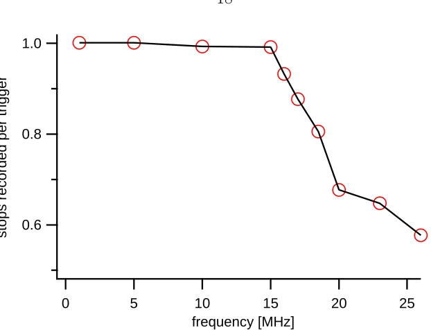
Figure 2.7: Measured probability of counting a “stop”, given a trigger, for the P7888 data acquisition card, as a function of the input RF frequency.

as suggested by Fig. 2.3.

One also needs to consider the effects of the imperfect registration between the FORT and the probe sinusoidal patterns inside the cavity. The mode order at λ_FORT

is even (see Sec. 4.1), so that the spatial dependence of the FORT depth on the axial coordinate z is sin2(2πz/λ_FORT), where we took the cavity center to be located at

z = 0. At λD2 however, the mode order is odd, so that the strength of the CQED

interaction g goes like cos(2πz/λD2), as shown in Fig. 2.6. Thus if the FORT and

DS345 VCO POS-200 ATTEN HAT-2 SPL ZSCJ-2-1 CPL ZDC-15-2 AMP ZHC-1-2W ATTEN HAT-4 SPEC E4411B AOM TEM-200-50 DIV SP8655A LP BLP-21.4 ATTEN HAT-6 & 12

SWITCH ZYSWA-2-50DR

AMP AU-1442

P7888 Ch. 3 & 4 Probe TTL ATTEN HAT-3 TTL ADWIN Sweep TTL

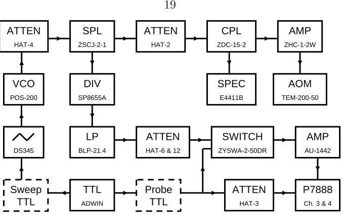
Figure 2.8: Electronics setup for digitizing the probe frequencyin situ.

depending on the temperature (wider for the hotter atoms), which should further broaden the vacuum-Rabi sidebands.

2.4

Experimental details

1.2

1.0

0.8

0.6

0.4

0.2

0.0

calibration factor

-80 -60 -40 -20 0 20 40 60

probe detuning [MHz]

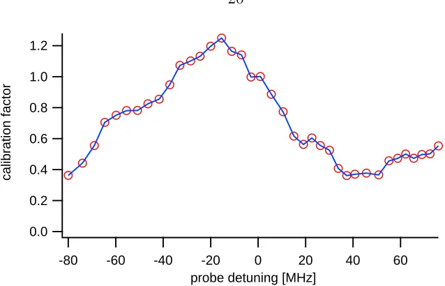
Figure 2.9: Normalization curve for detected probe power, as a function of detuning from atomic resonance.

One remaining technical challenge involved scanning the probe frequency in a controllable way. In order to cover a ∼140 MHz range around the atomic resonance, we needed to scan the RF supply to one of the double-passed AOMs that the probe goes through, in a range roughly from 135 to 205 MHz. Since we wanted the option of doing that scan several times a second, we decided for a POS-200 voltage-controlled oscillator (VCO) as the RF source, because VCOs can cover a large frequency range of 100 MHz or more, and they can do it fast, albeit not quite linearly with the input voltage. We used the P7888 pulse counting card that does our data acquisition to measure the VCO frequency in situ. As shown in Fig. 2.7, when connected to our 2.8 GHz Pentium IV computer, the card can count the pulses in an RF signal of up to 15 MHz with less than 1% error, but it drops a significant fraction of the triggers for larger input frequencies1. To bridge the gap between the VCO frequency and the computer card, we employed a ÷32 frequency divider chip, as shown schematically in Fig. 2.8. Note that we only acquire the divided frequency during those intervals when the probe is on (see Fig. 2.10), which gives the P7888 card enough time in between to write the pulses to the hard drive. Both the physics cavity and the probe are independently locked to Cesium, which means that once the probe AOM frequency

Probe Detuning

[MHz]

1.2 +70

-70 time [s]

0

Probing: probe: 4ĺ5’ repump: 3ĺ4’

0.1 ms

...

...

Cooling: radial: 4ĺ4’ axial: Raman

2.9 ms

...

...

Figure 2.10: Timing diagram for the vacuum-Rabi experiment.

is known, so are the cavity-probe and atom-probe detuning.

Another issue is related to the AOM resonance curve, which makes the input power to the cavity change as the probe frequency is being scanned. In addition, as the frequency changes, so does the probe beam alignment after the AOM, hence its coupling efficiency to the cavity. Both these effects can be however easily taken into account by acquiring a calibration curve, analogous to that from Fig. 4.3, and using it to normalize all probe spectra. At each point, for a particular probe detuning from the D2 line, the cavity is tuned to be in resonance with the light, and its transmission is recorded with the avalanche photodetectors. The calibration curve2 _{we took for}

the vacuum-Rabi experiment is shown in Fig. 2.9.

For acquiring the vacuum-Rabi spectrum3 _{of Sec. 2.5, the probe, the FORT and}

the locking laser all have the same linear polarization, perpendicular to that of the Raman beam, all set by the glan-laser polarizer angle at the cavity input. The probe polarization is close to one of the birefringent axes, namely to the one with the higher resonance frequency (the “blue” mode). The λ/2 waveplate at the cavity output is set so as to maximize the empty cavity (i.e., no atom present) probe transmission on

20

10

0

transmission [arb]

-60 -30 0 30 60

probe detuning [MHz]

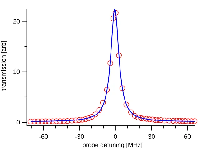
Figure 2.11: Empty cavity data acquired with the probe scanning protocol of Sec. 2.5. Fit yieldsκ = 2π×4.1 MHz.

resonance. After each trap loading attempt, we scan the probe frequency, while at the same time shuttering it on and off, in order to intersperse the cooling intervals. The timing diagram for the experiment is shown schematically in Fig. 2.10, and will be described in more detail in the next section. During each 100µs probing interval, both the probe and its repumper are turned on. We chose the F = 3 → F = 4 transition frequency for the repumper, because it has no dark states, hence it is an effective way to maximize the time the atom spends in the cavity-coupled, hence useful F = 4 state. Shuttering for all beams is done with RF switches at the AOM inputs. The FORT beam is on all the time.

2π×3.3 to 3.6 MHz in Chapter 4, as opposed to 4.1 MHz in Sec. 2.5. The latter value was determined by fitting a Lorentzian to empty cavity data obtained in the same manner as the vacuum-Rabi spectrum data, as shown in Fig. 2.11. More specifically, the probe frequency was scanned linearly over the ∼ 137 MHz range eight times in 1.2 s, and the resulting transmission spectra were averaged, then normalized by the curve shown in Fig. 2.9. The fit givesκ= 2π×(4.08±0.03) MHz for the Lorentzian half-width.

2.5

Observation of the vacuum-Rabi spectrum for

one trapped atom

This section is reproduced almost verbatim from Ref. [7].

A cornerstone of optical physics is the interaction of a single atom with the elec-tromagnetic field of a high quality resonator. Of particular importance is the regime of strong coupling, for which the frequency scalegassociated with reversible evolution for the atom-cavity system exceeds the rates (γ, κ) for irreversible decay of atom and cavity field, respectively [16]. In the domain of strong coupling, a photon emitted by the atom into the cavity mode is likely to be repeatedly absorbed and re-emitted at the single-quantum Rabi frequency 2g before being irreversibly lost into the environ-ment. This oscillatory exchange of excitation between atom and cavity field results from a normal mode splitting in the eigenvalue spectrum of the atom-cavity system [13, 17, 18], and has been dubbed the vacuum-Rabi splitting [17].

[22, 23, 24] and microwave regimes [25]. The combination of laser cooled atoms and large coherent coupling has enabled the vacuum-Rabi spectrum to be obtained from transit signals produced by single atoms [26]. A significant advance has been the trapping of individual atoms in a regime of strong coupling [27, 2], with the vacuum-Rabi splitting first evidenced for single trapped atoms in Ref. [27] and the entire transmission spectra recorded in Ref. [28].

Without exception these prior single atom experiments related to the vacuum-Rabi splitting in cavity QED [22, 25, 23, 24, 26, 27, 2, 28] have required averaging over trials with many atoms to obtain quantitative spectral information, even if individual trials involved only single atoms (e.g., 105 atoms were required to obtain a spectrum in Ref. [25] and > 103 _{atoms were needed in Ref. [28]). By contrast, the implementation}

of complex algorithms in quantum information science requires the capability for repeated manipulation and measurement of an individual quantum system, as has been spectacularly demonstrated with trapped ions [29, 30] and recently with Cooper pair boxes [31, 32].

With this goal in mind, we describe here measurements of the spectral response of single atoms that are trapped and strongly coupled to the field of a high finesse opti-cal resonator. By alternating intervals of probe measurement and of atomic cooling, we record a complete probe spectrum for one and the same atom. The vacuum-Rabi splitting is thereby measured in a quantitative fashion for each atom by way of a protocol that represents a first step towards more complex tasks in quantum infor-mation science. An essential component of our protocol is a new Raman scheme for cooling atomic motion along the cavity axis, that leads to inferred atomic localization ∆z_axial 33 nm, ∆ρ_transverse 5.5 µm.

A simple schematic of our experiment is given in Fig. 2.12 [1], showing a single atom trapped inside our optical cavity in the regime of strong coupling by way of an intracavity far-off-resonance trap (FORT) driven by the fieldE_FORT. The transmission spectrum T₁(ωp) for the atom-cavity system is obtained by varying the frequency

Figure 2.12: Schematic of the vacuum-Rabi experimental setup.

while axial cooling results from Raman transitions driven by the fieldsE_FORT,E_Raman. An additional transverse field Ω₃ acts as a repumper during probe intervals.

After release from a magneto-optical trap (MOT) located several mm above the Fabry-Perot cavity formed by mirrors (M₁, M₂), single Cesium atoms are cooled and loaded into the intracavity FORT and are thereby strongly coupled to a single mode of the cavity. Our experiment employs the 6S₁/2, F = 4 →6P3/2, F = 5 transition of

the D2 line in Cesium atλA= 852.4 nm, for which the maximum single-photon Rabi frequency is 2g₀/2π = 68 MHz for (F = 4, mF = ±4) → (F = 5, mF = ±5). The transverse decay rate for the 6P₃/2 atomic states isγ/2π = 2.6 MHz, while the cavity

field decays at rate κ/2π = 4.1 MHz. Hence our system is in the strong coupling regime of cavity QED g₀ (γ, κ) [16].

trapping potential for these states isU₀/h=−39 MHz for all measurements presented in this section. Zeeman states of the 6P₃/2, F = 5 manifold likewise experience a

trapping potential, albeit with a weak dependence on m_F [2]. Birefringence in the mirrors leads to two nondegenerate cavity modes with orthogonal polarizations ˆl_±and mode splitting ∆νC₁ = 4.4±0.2 MHz at 852 nm. The fields EFORT and ERaman are

linearly polarized and aligned close to the two orthogonal polarizations ˆl₊ and ˆl₋ of the higher, respectively the lower frequency mode. The cavity length is independently stabilized to length l₀ = 42.2 µm such that a T EM₀₀ mode at λC1 is resonant with the free-space atomic transition at λA and another T EM00 mode at λC₂ is resonant at λF. At the cavity center z = 0, the mode waists are wC1,2 = {23.4,24.5} µm at

λC_1,2 ={852.4,935.6}nm.

As illustrated in Fig. 2.12, we record the transmission spectrum T₁(ωp) for a weak external probe Ep of variable frequency ωp incident upon the cavity containing one strongly coupled atom. T₁(ωp) is proportional to the ratio of photon flux transmitted byM₂to the flux|Ep|2_{incident uponM}

1, with normalizationT0(ωp =ωC₁)≡1 for the empty cavity. Our protocol consists of an alternating sequence of probe and cooling intervals. The probe beam is linearly polarized and is matched to the T EM₀₀ mode around λC1. Relative to ˆl±, the linear polarization vector ˆlp for the probe field Ep is aligned along a direction ˆlp = cosθˆl++ sinθˆl−, whereθ = 13◦ for Fig. 2.13; however,

the theoretical model we will discuss below maintains that the spectrum is relatively insensitive to θ for θ 15◦. The probe field Ep illuminates the cavity for ∆t_probe = 100 µs, and the transmitted light is detected by photon counting. The efficiency for photon escape from the cavity is αe2 = 0.6±0.1. The propagation efficiency

from M₂ to detectors (D₁, D₂) is αP = 0.41±.03, with then each detector receiving half of the photons. The avalanche photodiodes (D₁, D₂) have quantum efficiencies

αP = 0.49±0.05. During each probing interval a repumping beam Ω3, transverse to

the cavity axis and resonant with 6S₁/2, F = 3→6P3/2, F = 4, also illuminates the

2 4

-40 0 40

Probe Detuning ω_p (MHz)

-40 0 40

2 4 〈n(_ω

p₎

〉 ×

10

-2

2 4

0.3

0.2

0.1

0.0 0.3

0.2

0.1

0.0

T1

(

ωp

)

0.3

0.2

0.1

0.0

Figure 2.13: Transmission spectrum T₁(ωp) for six randomly drawn atoms, and steady-state solution to the master equation, for comparison.

initiated.

Following each probe interval, we apply light to cool both the radial and axial motion for ∆t_cool = 2.9 ms. Radial cooling is achieved by the Ω₄ beams consisting of pairs of counter-propagating fields in a σ_± configuration perpendicular to the cavity axis, as shown in Fig. 2.12. The Ω₄ beams are detuned ∆₄ 10 MHz to the blue of the 4 → 4 transition to provide blue Sisyphus cooling [15] for motion transverse to the cavity axis.

transitions between the F = 3,4 levels with effective Rabi frequency ΩE ∼ 200 kHz. By tuningδnear the ∆n=−2 motional sideband (i.e.,−2ν₀ ∼δ=−1.0 MHz, where

ν₀ is the axial vibrational frequency at an antinode of the FORT), we implement sideband cooling via the F = 3 → 4 transition, with repumping provided by the Ω₄ beams. The Raman process also acts as a repumper for population pumped to the

F = 3 level by the Ω₄ beams. Each cooling interval is initiated by turning on the fields Ω₄,E_Raman during ∆t_cool and is terminated by gating these fields off before the next probe interval ∆t_probe.

Fig. 2.13 displays normalized transmission spectra T₁ and corresponding intra-cavity photon numbers n(ωp) for six randomly drawn individual atoms, acquired via our protocol of alternating probe and cooling intervals. In each case, T₁(ωp) is obtained for one-and-the-same atom, with the two peaks of the vacuum-Rabi spec-trum clearly evident. The error bars reflect the statistical uncertainties in the number of photocounts. Also shown is the predicted transmission spectrum obtained from the steady-state solution to the master equation for one atom strongly coupled to the cavity, as discussed below. The quantitative correspondence between theory and experiment is evidently quite reasonable for each atom. Note that mF-dependent Stark shifts forF = 5 in conjunction with optical pumping caused by Ep lead to the asymmetry of the peaks in Fig. 2.13 via an effective population-dependent shift of the atomic resonance frequency. The AC-Stark shifts of the (F = 5, m_F) states are given by{m_F, Um_F}={±5,1.18U},{±4,1.06U},{±3,0.97U},{±2,0.90U}, {±1,0.86U}, and {0,0.85U}.

To obtain the data in Fig. 2.13, N_load = 61 atoms were loaded into the FORT in 500 attempts, with the probability that a given successful attempt involved 2 or more atoms estimated to be P_load(N ≥2)0.06. Of the N_load atoms,N_survive = 28 atoms remained trapped for the entire duration ∆t_tot. The six spectra shown in Fig. 2.13 were selected by a random drawing from this set ofN_survive atoms. Our sole selection criterion for presence of an atom makes no consideration of the spectral structure of

T₁(ωp) except that there should be large absorption on line center, T1(ωp = ωC₁) ≤

1 2 3 4

〈

n(

ω

p₎

〉 ×

10

-2

-60 -40 -20 0 20 40 60

Probe Detuning ω_p (MHz) 0.35

0.30

0.25

0.20

0.15

0.10

0.05

0.00

T1

(

ωp

)

individual atoms average of atoms steady state theory, 30 wells, k

B

T

Figure 2.14: Individual transmission spectraT₁(ωp) (dots), their average ¯T1(ωp) (thick trace), and the steady-state solution to the master equation (thin trace).

selection criteria 0.02≤ T_thresh ≤ 0.73. Note that an atom trapped in the FORT in the absence of the cooling and probing light has lifetime τ₀ 3 s, which leads to a survival probability p(∆t_tot) 0.7.

In Fig. 2.14 we collect the results for T₁(ωp) for all Nsurvive = 28 atoms, and

only 40 ms.

We have also acquired transmission spectra T₁(ωp) for operating conditions other than those in Figs. 2.13 and 2.14, including intensities |Ep|2 _{varied by factors of 2,} 1

2,

and 1₄, and atom-cavity detunings ∆AC = ωA−ωC1 = ±13 MHz. We will describe these results elsewhere.

The full curves in Figs. 2.13, 2.14 are obtained from the steady state solution of the master equation including all transitions (F = 4, mF)↔(F = 5, mF) with their respective coupling coefficients g(mF,mF)

0 , as well as the two nearly degenerate modes

of our cavity. For the comparison of theory and experiment, we reemphasize that the parameters (g(mF,mF)

0 , γ, κ,∆AC, ωp −ωA,∆νC1,|Ep|2, U0) are known in absolute

terms without adjustment. However, we have noa priori knowledge of the particular FORT well into which the atom is loaded along the cavity standing wave, nor of the energy of the atom. The FORT shift and coherent coupling rate are both functions of atomic positionr, with

U(r) =U₀sin2(kC₂z) exp(−2ρ2/wC22), (2.18)

g(mF,m_F)_{(r) =g}(mF,m_F)

0 ψ(r), (2.19)

where g₀(mF,mF) = g₀Gm_F,m_F with Gi,f related to the Clebsch-Gordan coefficient for the particular mF ↔mF transition. Here

ψ(r) = cos(kC₁z) exp(−ρ2/w2C₁), (2.20)

0.4 0.3 0.2 0.1 0.0 T1 ( ωp )

-60 -40 -20 0 20 40 60

Probe Detuning ω_p (MHz) k

B

T

-60 -40 -20 0 20 40 60

Probe Detuning ω_p (MHz) # of wells

1 30 60 90 k

B

T

10

0

# of wells

1.0 0.5

0.0

|ψ(r_FORT)| (a)

(b)

Figure 2.15: Theoretical plots forT₁(ωp): (a) zero temperature, spectrum dependence on probe-FORT registration; (b) perfect registration, dependence on temperature.

experiment allows us to infer that our cooling protocol together with the selection criterion T_thresh= 0.2 results in individual atoms that are strongly coupled in one of the “best” FORT wells (i.e., |ψ(r_FORT)| 0.87) with “temperature” ∼ 200 µK. In Figs. 2.13 and 2.14, the discrepancy between experiment and the steady-state theory for ¯T₁(ωp) around ωp ∼0 can be accounted for by a transient solution to the master equation which includes optical pumping effects over the probe interval ∆t_probe. Also, although the spectra are consistent with a thermal distribution, we do not exclude a more complex model involving probe-dependent heating and cooling effects.

predicted by the steady-state solution of the master equation is calculated from an average over various FORT antinodes along the cavity axis, with the inset showing the associated distribution of values for |ψ(r_FORT)|. Extending the average beyond the 30 “best” FORT wells leads to spectra that are inconsistent with our observations in Figs. 2.13 and 2.14. Fig. 2.15 (b) likewise investigates the theoretical dependence ofT₁(ωp) on the temperatureT for an atom at an antinode of the FORT with optimal coupling (i.e., |ψ(r)| = 1). Now T₁(ωp) is computed for various temperatures from an average over atomic positions within the well. For temperatures T 200 µK, the calculated spectra are at variance with the data in Figs. 2.13 and 2.14, from which we infer atomic localization ∆z 33 nm in the axial direction and ∆x= ∆y 3.9 µm in the plane transverse to the cavity axis. Beyond these conclusions, a consistent feature of our measurements is that reasonable correspondence between theory and experiment is only obtained by restricting |ψ(r)|0.8.

Chapter 3

Dark-mode up-goers and photon

blockade

This chapter describes our recent experiment studying the photon statistics of light transmitted by the atom-cavity system when driven on the red vacuum-Rabi side-band. We start by introducing a simple theoretical model justifying the non-classical character of the emitted light field, and then we describe the experimental protocol and data analysis method in detail. We conclude by discussing the experimental re-sults, including the observation of sub-Poissonian and anti-bunched photon statistics, as well as motional effects leading to an estimate of the atomic temperature.

3.1

Master equation, revisited

Let us go back to the simple theoretical model describing a two-level atom strongly coupled to a single cavity mode (see Sec. 2.1 and 2.2). Recalling the Jaynes-Cummings picture in Fig. 2.1, we see that the |±₁ states are separated by 2g, whereas the |±₂ splitting is 2√2g. Now suppose that the probe laser frequency is tuned to resonance with one of the vacuum-Rabi sidebands, say the red one at

ωP = ωA−g. If the system is excited to the |−1 state, then the anharmonicity of

sup-pressed. One can think of this as a “photon blockade,” in the sense that absorption of the first photon from an incoming Poissonian stream will block the absorption of a second one, leading to sub-Poissonian statistics in the output field. It can be shown (see e.g., Ref. [34], Sec. 12.10.3) that if the photon statistics for a light field are sub-Poissonian, the state of that field cannot be described by a classical probability functional. Hence, this state is interesting, from a quantum optics perspective.

For a more quantitative description of what is going on, let us consider the corre-lations between pairs of photons transmitted by the driven atom-cavity system. We will compute here the zero-delay second-order intensity correlation function g(2)_(0),

in the case of weak driving. Obviously the truncated three-state basis of Sec. 2.2 is insufficient for observing coincidences, so we will enlarge the state space to allow for two quanta of energy as well: {|g,0,|g,1,|e,0 |g,2,|e,1}. The Hamiltonian and master equation are still those from Eqns. (2.8) and (2.9), which we used in Chapter 2 to derive the vacuum-Rabi spectrum.

In this five-state basis, the only non-zero matrix elements for the relevant operators are:

g,1|a†σ₋|e,0 =e,0|aσ₊|g,1 = 1 g,2|a†σ₋|e,1 =e,1|aσ₊|g,2 = √2

e,0|σ₊σ₋|e,0 =e,1|σ₊σ₋|e,1 = 1 (3.1) g,1|a†a|g,1 =e,1|a†a|e,1 = 1

g,2|a†a|g,2 = 2.

Also, for weak driving E/κ1, the density operator for the atom-cavity system is of the form

ρ=|ψψ|, (3.2)

that is, despite dissipation, the system can be described by a pure state [35, 36]:

where the single and double excitation components scale linearly and quadratically, respectively, with the drive strength:

a₁, a₂ ∝ E

κ a3, a4 ∝

E κ

₂

, (3.4)

so that |ψ is normalized to first order in the drive strength. We can now use the master equation for ρ to derive equations of motion for the a₁₋₄ coefficients. From the first column of the Liouvillian, keeping only terms to leading order in the drive parameter E/κ, we have:

˙

a₁ = −(κ+iδCP)a1 −iga2−iE

˙

a₂ = −iga₁−(γ+iδAP)a2

˙

a₃ = −i√2Ea₁−2(κ+iδCP)a3−i

√

2ga₄ (3.5)

˙

a₄ = −iEa₂−i√2ga₃−(γ+iδAP)a4−(κ+iδCP)a4.

Note that the first two equations in (3.5), describing the evolution of a₁ and a₂, are identical to Eqns. (2.14) for α =a and β = σ₋, which is not surprising since to first order in E/κ, α=a₁ and β =a₂.

If all we are interested in is computing g(2)_{(0), then we only need the steady state}

solution, which we get by setting the left hand side of all equations in (3.5) to zero:

ass₁ = −iEγ˜

g2_{+ ˜κγ˜}

ass₂ = −Eg

g2_{+ ˜κγ˜}

ass₃ = E

2_(g2 _{−γ˜(˜κ+ ˜γ))}

√

2(g2_{+ ˜κγ˜)(g}2_{+ ˜κ(˜κ+ ˜γ))} (3.6)

ass₄ = iE

2_{g(˜κ+ ˜γ)}

(g2_{+ ˜κγ˜)(g}2_{+ ˜κ(˜κ+ ˜γ))} ,

where we have defined ˜κ ≡ κ+iδCP and ˜γ ≡ γ +iδAP. Note that all a1−4

10-1 100 101 102 103 104

g

(2)

(0)

probe detuning [MHz]

Matlab calculation analytic expression

0

-g g

Figure 3.1: g(2)(0) as a function of probe detuning from the atomic resonance.

operators.

The second-order normalized intensity correlation function at zero delay is by definition given by

g(2)(0) = a

†2_a2

a†a2 , (3.7)

where the expectation value is to be taken in the steady state |ψss _{as set by Eqns.} (3.6). Given the known scaling with the drive parameter from Eqn. (3.4), we find:

g(2)(0) = 2|a ss

3 |2

(|ass

1 |2+ 2|ass3 |2+|ass4 |2)2

2|ass

3 |2

|ass

1 |4

, (3.8)

which for small E is independent of the driving strength.

This derivation was done with the help of Mathematica [37], and in the most part following Refs. [35, 36], which deal with the more general, many-atom case, and with delayed coincidences. These papers also have a different phase convention for a and

a†, and a somewhat less algebra-intensive way of obtaining the steady-state solution, namely by first settingδCP =δAP = 0 in the Hamiltonian, and then only for the final result making the formal substitutionsκ→κ˜and γ →γ˜(note the typo in Eqn. (38) of Ref. [36]).

Now we can evaluateg(2)_{(0), by plugging experimentally relevant parameter values}

detuning from atomic resonance, for g = 2π× 34 MHz, κ = 2π ×4.1 MHz, γ = 2π × 2.6 MHz, and δCP = δAP. Note in the region near δCP = δAP = ±g, the curve dips below the dashed line at unity, i.e., g(2)_{(0) < 1, reaching a minimum of}

g(2)(0) 0.27. This means that if we drive the atom-cavity system on either of the two vacuum-Rabi sidebands (recall Fig. 2.2), the emerging photon stream will exhibit sub-Poissonian statistics. This is precisely what we implied in the intuitive discussion at the beginning of this section.

Fig. 3.1 also shows the result of a numerical Matlab [38, 39] calculation1, using Kevin Birnbaum’s jaynescummings w suffix.m script [9]. The code uses a truncated six-state space {|g,|e} ⊗ {|0,|1,|2}, and a drive strength of E/κ = 0.01 (empty cavity photon number on resonance (E/κ)2 _{= 10}−4_{). Note that the two curves in Fig.}

3.1 represent nearly the same weak-field approximation, so not surprisingly they are very close (almost indistinguishably so in the log-scale figure), differing by at most 5% over the entire range of possible detunings.

The experimental results we present in Sec. 3.6 show that the photon stream emerging from our real-life atom-cavity system also has manifestly non-classical statis-tics near the red vacuum-Rabi sideband, as evidenced by the sub-Poissonian and anti-bunched character of the detected light. The model which quantitatively predicts a value for g(2)_{(0) consistent with what we observe in the lab is rather complicated [9].}

However, our simple model presented above is sufficient to predict the qualitative behavior of the system, namely the non-classical character of the photon statistics at the cavity output.

1_{This curve also appears in Sec. 3.6 Fig. 3.16 (a), for slightly different parameters g = 2π×}

(a) (b)

Figure 3.2: Second-order normalized intensity correlation function for (a) a constant signal; (b) a square pulse.

3.2

Turning coincidences into

g

(

τ

)

The normalized second-order intensity correlation function corresponding to a classi-cal field of intensity I(t) is defined as

g(2)(t, τ) = I(t)I(t+τ)

I(t)I(t+τ), (3.9)

where the brackets denote ensemble averages. Often one deals with stationary processes, for which the ensemble averages do not depend on the origin of time, making g(2)(t, τ) is a function of τ alone. Also, the field is usually ergodic, meaning that ensemble averages can be replaced by averages over all time:

I(t)I(t+τ) = lim T→∞

1

T

T /2

−T /2

I(t)I(t+τ) dt

I(t)=I(t+τ) = lim T→∞

1

T

T /2

−T /2

I(t) dt . (3.10)

For times long compared with the coherence time of the signal, the numerator in Eqn. (3.9) factorizes, so that the normalized intensity correlation function asymptotes to unity:

I(t)I(t+τ)=I(t)I(t+τ) =⇒ g(2)(τ → ∞) = 1. (3.11)

The trouble with this picture is that one cannot sample a signal for all time; rather, one would typically measure it for a finite interval of lengthT₀, and construct signal averages in the following way:

I(t)I(t+τ)T₀ = 1

T₀

T₀/2

−T0/2

I(t)I(t+τ) dt

I(t)T₀ =I(t+τ)T₀ = 1

T₀

T0/2

−T0/2

I(t) dt, (3.12)

where the corresponding normalized correlation function is

g_T(2)

0(τ) =

I(t)I(t+τ)T₀ I(t)2

T0

. (3.13)

Here |τ|< T₀, and I(t) is assumed to be non-zero only in the interval [−T₀/2, T₀/2]. How is thisg(2)_T

0(τ) related to the correlation function for the stationary process that is being sampled, i.e., to g(2)(τ) evaluated in the intervalτ ∈[−T₀, T₀]? The example of constant intensity we considered above now becomes a square pulse, withI(t) = I₀ for |t|< T₀/2, and zero elsewhere. From (3.13), we find that the finite-interval correlation function is

g_T(2)₀(τ) = 1− |τ|/T₀. (3.14) Thus the finite sampling time has the effect of putting a triangular shape on an inherently constant correlation function, as shown in Fig. 3.2. Because of that, one will often compensate for this triangle effect, by multiplying a measured correlation function by the factor T₀/(T₀ − |τ|). The result then has the asymptotic behavior one would expect from a stationary process (see Eqn. 3.11), albeit with increasing fluctuations as we near |τ|=T₀ where the multiplication factor diverges.

j =−N + 1, . . . , N −1. The discretized version of Eqn. (3.12) is:

I(t)I(t+τ)N = 1

N

N

k=1

akak+j

I(t)N =I(t+τ)N = 1

N

N

k=1

ak, (3.15)

with normalized intensity correlation function given by

g_N(2)(τ) = I(t)I(t+τ)N I(t)2

N

. (3.16)

Ideally one single-photon detector would suffice for measuring the autocorrelation of the incoming light field. However, real detectors have non-trivial autocorrelations (see Sec. 2.3.1 of Ref. [1]). First, there is the dead time: after recording a photocount, our detectors take about τDT = 53 ns to recover before they can detect the next photon. This means that if one is interested in correlations for times shorter than the dead time|τ|< τDT, one needs two detectors. Secondly, there is the problem of after-pulsing, whereby about 1.2% of the time, the detector records not one, but two counts per incoming photon. This means that, for accurate field intensity autocorrelation measurements, one should only consider the cross-correlation of the click times coming from two different detectors, and ignore those coincidences corresponding to one and the same detector.

By extension of the single-detector picture, let the number of clicks in the kth

bin coming from each of the two detectors be ak and bk. Then Eqn. (3.15) can be updated for the two-detector, cross-correlation case:

IA(t)IB(t+τ) = 1

N

N

k=1

akbk+j

IA(t) = 1

N

N

k=1

ak (3.17)

IB(t) = 1

N

N

k=1