An elliptic optimal control problem and its two relaxations

An Elliptic Optimal Control Problem and its Two Relaxations

Behrouz Emamizadeh

Faculty of Science and Engineering The University of Nottingham Ningbo, China

[email protected]

Amin Farjudian

Center for Research on Embedded Systems Halmstad University, Sweden

[email protected]

Hayk Mikayelyan

Faculty of Science and Engineering The University of Nottingham Ningbo, China

[email protected]

July, 2016

Abstract

In this note, we consider a control theory problem involving a strictly convex energy functional, which is not Gˆateaux differentiable. The functional came up in the study of a shape optimization problem, and here we focus on the minimization of this functional. We relax the problem in two different ways, and show that the relaxed variants can be solved by applying some recent results on two-phase obstacle like problems of free boundary type. We derive an important qualitative property of the solutions, i. e., we prove that the minimizers are three-valued, a result which significantly reduces the search space for the relevant numerical algorithms.

Key Words:Minimization, Free boundary, Optimality condition, Non-smooth analysis

Mathematics Subject Classification:49J20, 35R35

1

Introduction

We consider the minimization of a functional, which has been studied in the context of two-phase membrane problem by several authors [1–3]. In [1], the relation between the minimization problem and optimal control theory has been mentioned.

The functional is strictly convex, but not Gˆateaux differentiable, and we minimize the functional over suit-able admissible sets. Using the recent results from the theory of free boundary problems, we prove that the solutions satisfy an important qualitative property. Specifically, we prove that the minimizers are three-valued, a result which reduces the search space for any numerical solution of the problem from a large function space to a more manageable space of three-valued functions.

In what follows, we present the formal statement of the main results in Section 2. The tools and preliminary results form the content of Section 3, which is followed by the proofs of the two main theorems of the paper in Sections 4 and 5. Section 6 contains the conclusions.

∗

2

Statement of the Main Results

As already mentioned, this note is concerned with the minimization of a strictly convex energy functional, which fails to be Gˆateaux differentiable. The functional,Φ:W1,2(D)→_R, is defined by:

Φ(u)B 1

2

Z

D

|∇u|2dx+

Z

D

|u|dx− Z

∂Dψu dσ,

in which D ⊆ _RN, andψ ∈ L2(∂D) satisfies R_∂Dψdσ = 0. We will consider the minimization problem over three admissible sets.

First, defineWB

n

u∈W1,2(D) :R_Du dx=0o, and let:

F_1B

(

f ∈L∞(D) :∀x∈D:−1≤ f(x)≤1, Z

D

f dx=0

)

, (2.1)

F_2B

(

f ∈L∞(D) : sup_x∈Df −infx∈Df ≤2,

Z

D

f dx=0

)

. (2.2)

Observe thatF₁⊂ F₂. For each f ∈ F₂, we use the notationS(f) to denote the set of solutions of the following Neumann boundary value problem:

      

−∆u= f inD,

∂u

∂ν =ψ on∂D,

(2.3)

and we define:

      

K_{1 B} S

f∈F1S(f), P(K1) B W∩K1,

      

K_{2 B} S

f∈F2S(f), P(K2) B W∩K2.

Remark 2.1. If we use the divergence theorem on (2.3), we will get the compatibility condition R_D f dx =

−R_∂Dψdσ. As we had already assumed thatR_∂Dψdσ=0, we requiredf to satisfyR_D f dx=0 in the definitions ofF1andF2in (2.1) and (2.2), respectively.

Remark2.2. It is well known that the setG_B{g∈L∞(D) : 0 ≤g ≤1, R

Dg dx=α}is theσ(L

∞_,L1_)-closure

of the set

G0B{χE :Eis a measurable subset ofDand|E|=α},

in whichχE is the characteristic function of the setE, and|E| is itsN-dimensional Lebesgue measure. Here,

σ(L∞,L1) denotes the w∗-topology onL∞(D). A straightforward argument proves that F1 is the σ(L∞,L1 )-closure of the set

F₁0B

(

χE −χEc :Eis a measurable subset ofDand|E|= 1

2|D|

)

.

The functions inF₁0 are{−1,1}-valued. As a result, they are sometimes referred to as ‘bang-bang’ functions. Interestingly, the minimizers of our problems are, in general, not bang-bang functions, and can have three values.

We are interested in the following three minimization problems:

inf

u∈P(K1)

Φ(u), (2.4)

inf

u∈K1

Φ(u), (2.5)

inf

u∈P(K2)

Φ(u). (2.6)

Our main results in this paper are the following two theorems:

Theorem 2.1. The minimization problem(2.5)has a unique solution u₀. Moreover:

(i) ∆u0 =χ{u0>0}−χ{u0<0},

(ii) |{u₀ <0}|=|{u₀>0}|,

where for any X⊆_RN_{, the notation|X|has been used for the N-dimensional Lebesgue measure of X.}

Proof. See Section 4, page 5.

Remark2.4. Note that the assertions (i) and (ii) in Theorem 2.1 imply thatu0 can be neither strictly positive nor strictly negative in the entire domainD.

Theorem 2.2. The minimization problem (2.6) has a unique solution v₀. Moreover, there exists a unique

constant h0∈]−1,1[, such that:

(i) ∆v0 =(1+h0)χ{v0>0}−(1−h0)χ{v0<0},

(ii) (1+h0)|{v0>0}|=(1−h0)|{v0 <0}|.

Proof. See Section 5, page 7.

It should be pointed out that the minimization problem (2.5) isnotan optimal control problem, where one minimizes a functional with respect to an admissible set of controllers and a partial differential state equation. Let us briefly explain this point. Suppose that f ∈ F₁, anduf is the unique solution of the boundary value

problem (2.3) for whichR_Duf dx=0; thus,uf ∈P(K1)⊂K1. As a result, we obtain:

inf

f∈F1

Φ(uf)= inf u∈P(K1)

Φ(u). (2.7)

IfR_Du0dx,0, whereu0is the unique solution of (2.5), then we have:

inf

f∈F1

Φ(uf)= inf u∈P(K1)

Φ(u)> inf

u∈K1 Φ(u).

The authors make theconjecturethat the solutionw₀of the minimization problem (2.4) is the projection ofu₀

ontoW. In other words, ifΦ(u0)=infu∈K1Φ(u), and

w0(x)BP(u0)(x)=u0(x)− 1

|D| Z

D

u0(x)dx,

thenΦ(w0)=infv∈P(K1)Φ(v).

Studying the minimization problems (2.5) and (2.6) was a natural task for us as we were attempting to construct solutions of the so-called two-phase obstacle like problem

∆u=λ₊χ{u>0}−λ−χ{u<0},

where λ± are positive Lipschitz functions, which we needed in our study of a shape optimization problem.

In [1], it has been proven that the free boundary of{u = 0}in a neighborhood of each branch point x ∈∂{u>

0} ∩∂{u < 0} ∩ {∇u= 0}is a union ofC1 graphs (also, see [2, 3]). This result helps us in drawing significant qualitative conclusions about the optimal shapes. An effective numerical method is presented in [4].

In what follows,k · kpdenotes the usualLp-norm,k · kp,∂Ddenotes theLp-norm on the boundary ofD, and

k · k denotes theW1,2-norm. Moreover, the symbolC will indicate various constants at different stages with

3

Preliminaries

In this section, we collect some tools which will help us in proving Theorems 2.1 and 2.2. We begin with the observation thatW = {u ∈ W1,2(D) : hu,1i = 0}, whereh·,·idenotes the inner product inW1,2(D). Hence, we can writeW1,2(D) as the direct sumW1,2(D) = WL_R. As a consequence, the projection P:W1,2(D) →

W1,2(D), with rangeR(P)=Wand null setN(P)=R, is well defined, and we have:

W1,2(D)=R(P)MN(P).

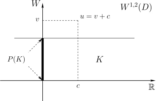
Whence, everyu∈W1,2(D) can be uniquely written asu=v+c, for somev∈Wandc∈_R.

Note that eachK ∈ {K1,K2}is a cylindrical set, in the sense thatK+R= K. This, in turn, implies that the

projectionP(K) ofKis contained inK, andK =P(K)LR. Fig. 1 provides an intuitive picture.

P(K)

_K

W

R

u=v+c v

c

W

(

D

)

Figure 1: The setW1,2(D), and its cylindrical subsetK ∈ {K1,K2}, can be written as the direct sumsW1,2(D)=

WL_RandK =P(K)LR, respectively.

Let us mention two more properties ofK1andK2:

Lemma 3.1. The sets K1, P(K1), K2, and P(K2), are convex and closed in W1,2(D).

Proof. First, note that bothF1andF2are convex sets:

∀f,g∈ F₁(or ∈ F₂), λ∈[0,1] :λf +(1−λ)g∈ F₁(or ∈ F₂).

This entails the convexity of K1 and K2 as for anyu1 ∈ S(f) and u2 ∈ S(g), we have: λu1+ (1−λ)u2 ∈

S(λf+(1−λ)g).

To prove closedness ofK₁, we consider a sequenceun ∈K1such thatun→uinW1,2(D). We need to show

thatu ∈ K1. Note that by definition, there exists a sequence (fn) ⊆ F1such that ∀n : un ∈ S(fn). Hence, the following integral equation holds for eachn:

Z

D

∇un· ∇w dx−

Z

∂Dψw dσ−

Z

D

fnw dx=0, ∀w∈W1,2(D). (3.1)

Since (fn) is bounded inL∞(D)'(L1(D))∗, we deduce that there is a subsequence—still denoted by (fn)—such

that fn →w∗ f in L∞(D). By the Banach-Alaoglu theorem,F₁ isw∗-compact, hencew∗-closed, and thereby

f ∈ F1. Returning to (3.1), and passing to the limit under the integrals, we obtain:

Z

D

∇u· ∇w dx− Z

∂Dψw dσ−

Z

D

f w dx=0, ∀w∈W1,2(D). (3.2)

From (3.2) we deduce thatu∈S(f). Hence,u∈K₁.

Closedness ofK2can be proved similarly. Closedness and convexity ofP(K1) andP(K2) follow from the

For the minimization problem (2.5) to make sense we need to make sure thatΦis bounded from below. In fact, it turns out thatΦis bounded from below throughoutW1,2(D), not just onK1orK2:

Lemma 3.2. The functionalΦis bounded from below on W1,2(D).

Proof. Everyu∈W1,2(D) can be written asu =v+c, for somev∈Wandc∈_R. Now, from the definition of

Φwe obtain:

Φ(u) ≥ 1

2

Z

D

|∇v|2dx− kψk_2,∂Dkvk_2,∂D

(trace embedding) ≥ 1

2

k∇vk2₂−Ckψk2,∂Dkvk

(Poincar´e) ≥ 1

2

k∇vk2₂−Ckψk₂,∂Dk∇vk2

≥ 1

2

k∇vk₂−C

2kψk2,∂D

2

− C

2

8 kψk 2 2,∂D

≥ −C

2

8 kψk 2

2,∂D. (3.3)

Note that the trace embedding that we have used is of type W1,2(D) → L2(∂D) (see, e. g., [5]). Clearly,

inequality (3.3) shows thatΦis bounded from below, as claimed.

4

Proof of Theorem 2.1

Proof. We begin with a minimizing sequence (un) ⊆ K1. Sinceun = vn+cn forvn ∈ P(K1) andcn ∈ R, and

R

∂Dψdσ=0, we have:

Φ(un)= 1 2

Z

D

|∇vn|2dx+

Z

D

|vn+cn|dx− Z

∂Dψvndσ. (4.1)

Note that:

Z

D

|vn+cn|dx ≥

Z

D

|cn|dx−

Z

D

|vn|dx

= |cn| |D| − kvnk₁

(L2,→L1) ≥ |cn| |D| −C1kvnk2

(Poincar´e and

Z

D

vndx=0) ≥ |cn| |D| −C2k∇vnk2, (4.2)

for some constantsC1andC2. Thus, using the trace embedding, Poincar´e inequality, and the fact that

R

Dvndx=

0, from (4.1) and (4.2) we infer:

Φ(un)≥ 1

2k∇vnk 2

2+|cn| |D| −Ck∇vnk2, (4.3)

for some constantC. Inequality (4.3), together with Lemma 3.2, implies that the real sequences (k∇vnk2) and (cn) are bounded. Thus, there existv0 ∈Wandc0∈Rsuch that for a subsequence—still denoted (un)—we have un *u0 =v0+c0inW1,2(D). By Lemma 3.1, the setK1is closed and convex. Thus, it is weakly closed and

u0 ∈K1. Due to the compact embeddingW1,2(D),→L2(D), a subsequence—still denoted by (un)—converges tou₀almost everywhere inD. As a result, we have:

(1) k∇v₀k₂ ≤lim infn→∞k∇vnk2, asW1,2-norm is weakly lower semi-continuous.

(2) R_D|u0|dx≤lim infn→∞ R

(3) limn→∞ R

∂Dψvndσ=

R

∂Dψv0dσ.

From (1), (2), and (3), we infer thatΦ(u₀) ≤ lim infn→∞Φ(un),which implies thatu0 solves the minimization problem (2.5). AsΦis strictly convex,u0is unique.

Interestingly,u0 is also the minimizer ofΦover the whole space W1,2(D). In fact, the solutionu∗ of the

minimization problem

inf

u∈W1,2(D)Φ(

u) (4.4)

is the solution of the so-called two-phase obstacle like problem with Neumann boundary data (see [3]):

      

∆u∗=χ{u∗>0}−χ{u∗<0} inD,

∂u∗

∂ν =ψ on∂D.

(4.5)

The right-hand sides of (4.5) must satisfy the compatibility condition

Z

D f∗dx=

Z

∂Dψdσ=0 (4.6)

for Neumann boundary value problems, where f∗ = −χ{u∗>0}+χ{u∗<0}. Moreover,−1 ≤ f∗ ≤ 1; thus, f∗ ∈ F1 andu∗∈K1. This means thatu∗=u0.

Theorem 2.1 (ii) follows from (4.6).

Remark4.1. The solutionu0 of the minimization problem (2.5) satisfies the differential equation −∆u0 = f0, where−f0=χ{u0>0}−χ{u0<0}is the right-hand side in the differential equation in (4.5). Whence, by local elliptic

regularity theory [6],u0 ∈W_loc2,p(D), for everyp∈]1,∞[. In particular, we deduce that the equation holds almost everywhere inD. By applying Lemma 7.7 in [7], we infer that the function f₀ must vanish on flat sections of the graph ofu0. Thus, f0must vanish on the set{u0=0}. This, in turn, implies that when|{u0=0}|is positive,

f0 cannot be an element of F₁0, as introduced in Remark 2.2. In other words, the function f0 may not be a bang-bang function, but a three-valued one.

Remark4.2. The optimality condition (4.5) can also be derived from 0∈∂Φ(u₀). Let us first decomposeΦas

Φ = Φ1+ Φ2−Φ3, in whichΦ1(u)B 1₂

R

D|∇u|

2_dx,Φ 2(u) B

R

D|u|dx, andΦ3(u)B

R

∂Dψu dσ. The functions Φ1andΦ3are Gˆateaux differentiable:

∂wΦ1(u0)=

Z

D

∇u₀· ∇w dx, ∀w∈W1,2(D), (4.7)

and

∂wΦ3(u0)=

Z

∂Dψw dσ, ∀w∈W

1,2_{(D). (4.8)}

However,Φ2is not globally Gˆateaux differentiable as its directional derivative at any pointuin the direction of

wis:

∂wΦ2(u)=

Z

{u,0}

sgn(u)w dx+

Z

{u=0} |w|dx,

where

sgn(x)B

          

1 (x>0),

0 (x=0),

−1 (x<0).

Hence, at anyu, the functionalΦ2is Gˆateaux differentiable only if|{u = 0}|= 0. Therefore,a priori, it is not known whetherΦ2—and as a resultΦ—will be Gˆateaux differentiable atu0or not.

The functionalΦ2, though not Gˆateaux differentiable, is Lipschitz inW1,2(D), as:

for some constantC. Therefore, the optimality condition satisfied byu0is:

0∈∂Φ(u0)+NK(u0), (4.9)

whereNK(u0) denotes the normal cone atu0 supported onK. Since K is convex (Lemma 3.1), we infer that

NK(u0) coincides with∂ξK(u0), in whichξKdenotes the indicator function supported onK(see, e. g., [8, 9]):

ξK(w)B

      

0, w∈K, +∞, w<K,

and

∂ξK(u0)=

n

g∈W1,2(D) :ξK(u)≥ξK(u0)+hg,u−u0i, ∀u∈W1,2(D)

o

. (4.10)

On the other hand:

∂Φ(u0)⊆∂Φ1(u0)+∂Φ2(u0)−∂Φ3(u0), (4.11)

since−Φ3is convex [8]. Whence, from (4.9) and (4.11) we obtain:

∇Φ1(u0)+γ− ∇Φ3(u0)+g=0 inW−1,2(D), (4.12)

for someγ∈∂Φ2(u0) andg∈∂ξK(u0). From (4.12) we obtain:

h∇Φ₁(u₀),u−u₀i+hγ,u−u₀i

− h∇Φ₃(u₀),u−u₀i+hg,u−u₀i=0, ∀u∈W1,2(D). (4.13)

At this stage, we use the fact that for convex and Lipschitz functionals∂Φcoincides with subdifferential (see Propositions 2.1.5 and 2.2.7 in [8]), to get:

hγ,u−u0i ≤∂u−u0Φ2(u0), ∀u∈W

1,2_{(D). (4.14)}

Now, from (4.13), (4.14), and (4.10), we deduce:

Z

D

∇u0·(∇u− ∇u0)dx−

Z

∂Dψ(u

−u0)dσ

+

Z

{u0,0}

sgn(u0)(u−u0)dx+

Z

{u0=0}

|u−u0|dx≥0, (4.15)

for everyu∈K. Note that in (4.15) we have usedξK(u)=ξK(u0)=0, because bothuandu0are inK. Equation (4.5) can be derived from (4.15), for which we refer the interested reader to [3].

5

Proof of Theorem 2.2

Proof. AsR_Du dx=0 foru∈W, overP(K₂)⊂W, minimization of the functional

Φ(u)= 1 2

Z

D

|∇u|2dx+

Z

D

|u|dx− Z

∂Dψ u dσ

is equivalent to minimization of the functional

Φh(u)B 1

2

Z

D

|∇u|2dx+

Z

D

(|u|+hu)dx− Z

∂Dψu dσ,

whereh∈[−1,1] is a parameter. Furthermore, we observe that the functionalΦhcan be written as:

Φh(u)= 1 2

Z

D

|∇u|2dx+

Z

D

((1+h)u++(1−h)u−)dx− Z

Let us now denote byuhthe unique solution of the minimization problem

inf

u∈W1,2(D)Φh(

u),

which is the solution of the following two-phase obstacle-like problem (see [3]):

      

∆uh=(1+h)χ{uh>0}−(1−h)χ{uh<0} inD, ∂uh

∂ν =ψ on∂D.

(5.2)

In what follows, we will prove three claims, which will lead to the existence of a uniqueh0∈]−1,1[, such thatuh₀ ∈W. This entails thatv0Buh0 is the unique solution of the minimization problem (2.6).

Claim 1. For allx∈D:u1(x)≤0 andu−1(x)≥0.

Proof. The functionu₁is the minimizer of the functional

Φ1(u)= 1 2

Z

D

|∇u|2dx+

Z

D

2u+dx− Z

∂Dψu dσ.

IfMBsupx∈Du1(x)>0, then the function ˜uBu1−Mwill have a smaller energy, i. e.,Φ1( ˜u)<Φ1(u1), which is a contradiction. The proof ofu−1≥0 is similar.

Claim 2. Ifh1>h2, then for allx∈D:uh1(x)≤uh2(x).

Proof. Let us assume thatD∗B{x∈D:uh1(x)>uh2(x)},∅, and take:

      

v1 Bmin(uh1,uh2),

v2 Bmax(uh1,uh2).

We haveΦh1(uh1) < Φh1(v1) andΦh2(uh2) < Φh2(v2). Adding up the two inequalities, and canceling out the

repeating terms on both sides, we obtain:

Z

D∗

(1+h1)u+h1+(1−h1)u

−

h1 +(1+h2)u

+

h2+(1−h2)u

−

h2dx<

Z

D∗

(1+h1)u+h2+(1−h1)u

−

h2 +(1+h2)u

+

h1+(1−h2)u

−

h1dx,

which can be written as:

(h₁−h₂)

Z

D∗

uh1dx=

Z

D∗

(h₁−h₂)(u+_h 1−u

−

h1)dx<

Z

D∗

(h1−h2)(u+h2 −u

−

h2)dx=(h1−h2)

Z

D∗

uh₂dx.

This is a contradiction.

Proof. Assume thathn → h0. Without loss of generality, we can assume thathn is monotone. The uniform convexity, coercivity, and lower semi-continuity of the family of functionals Φhn makes it possible to find a

convergent sub-sequenceun → v. In fact, because of monotonicity by the previous claim, we do not need to

take a sub-sequence.

Evidently,Φh0(uh0)≤Φh0(v)=limn→∞Φhn(un). On the other hand, from continuity ofΦhwith respect toh

andu, it follows that:

Φh0(uh0)≥lim inf_n→∞ Φhn(un)= Φh0(v),

since otherwiseΦh_n(u₀) < Φh_n(un) fornlarge enough. The convexity ofΦh0 and uniqueness of its minimizer

yield thatu0=v.

The three aforementioned claims prove the existence of the minimizer and item (i) of the theorem. Item (ii)

follows from the fact that the integral of∆v0vanishes.

6

Conclusions

Many optimization algorithms rely on the existence of gradient, which in the context of what we have presented in this paper, translates into Gˆateaux differentiability. The functional that we considered lacks this property, which makes any attempt at searching through the entire admissible function space extremely inefficient.

Yet, we proved that searching through the entire space is unnecessary as the solutions are bound to be three-valued. This reduces the search space significantly, and although the traditional gradient methods are not applicable, it is feasible to make use of other optimization methods to tackle the problem numerically.

References

[1] Shahgholian, H., Uraltseva, N., Weiss, G.S.: The two-phase membrane problem—regularity of the free boundaries in higher dimensions. International Mathematics Research Notices2007(2007)

[2] Emamizadeh, B., Prajapat, J.V., Shahgholian, H.: A two phase free boundary problem related to quadrature domains. Potential Analysis34(2), 119–138 (2010)

[3] Petrosyan, A., Shahgholian, H., Uraltseva, N.: Regularity of free boundaries in obstacle-type problems,

Graduate Studies in Mathematics, vol. 136. American Mathematical Society, Providence, RI (2012)

[4] Bozorgnia, F.: Numerical solutions of a two-phase membrane problem. Appl. Numer. Math.61(1), 92–107 (2011)

[5] Adams, R.A., Fournier, J.J.F.: Sobolev spaces, Pure and Applied Mathematics, vol. 140, second edn. Elsevier/Academic Press, Amsterdam (2003)

[6] Agmon, S.: The Lp approach to the Dirichlet problem. Part I : regularity theorems. Annali della Scuola

Normale Superiore di Pisa - Classe di Scienze13(4), 405–448 (1959)

[7] Gilbarg, D., Trudinger, N.S.: Elliptic Partial Differential Equations of Second Order. Springer-Verlag (2001)

[8] Clarke, F.H.: Optimization and Nonsmooth Analysis. Classics in Applied Mathematics. Society for Indus-trial and Applied Mathematics (1990)