StreamSVC: A New Approach To Cluster Large
And High-Dimensional Data Streams
Hasan Saberi, Mohammadali Mehdiaghaei
Abstract—The data stream mining has been studied ex-tensively in recent years. This paper is introducing a novel method to cluster high-dimensional data streams, based on famous SVC method, named StreamSVC. SVC projects the images of the data points in a high–dimensional feature space, to search for the minimal enclosing sphere, then classifies the points with respect to the distance between each point’s image and the central of feature sphere. In StreamSVC, for a single change in the data stream environment, the algorithm redoes the classification part. The algorithm involves only the parts of the data set which are affected during the change of stream and updates the classes in an appropriate time complexity order. Also, in order to update the clusters, in the stream process, we used some new improvements in the labeling piece of original SVC. These improvements are applied to reduce the computational costs for classification part and the cluster’s labeling piece. The experimental results show both time efficiency and high accuracy for large data streams.
Index Terms—Data stream, Clustering, SVC, Labeling piece.
I. INTRODUCTION
T
HE process of grouping a set of data points into classes of similar data is called clustering. Lately, advancing on technology and communication systems, the data sets in stream form are widely generated. They are temporally ordered, fast changing, massive, and potentially infinite. It may be impossible to store an entire data stream or to scan through it multiple times due to its tremendous volume. The critical issues are Data Stream Management Systems and Stream Queries. Such queries and managements requires accurate and time efficient stream analysis. Clustering and cluster analysis are major ways to analysis the data sets. Thus clustering of high dimensional data stream is now a famous concept in mining of data streams.There are some methodologies to deal with massive stream processing and stream systems. In order to handle these data types, some algorithm such as Random sampling, Sliding window or Histogram schemes are provided [1]. All of them get a part of total data set and reduces them into a abstracted data set. To obtain the clusters in a stream process, lots of researches have been performed [2], [3], [4], [5]. In the next section we introduce some of the new clustering approaches for data streams.
In (2001) Ben-Hur et al. [6] introduced SVC which is a kernel-based method for clustering massive and high– dimensional data sets. The algorithm applies a nonlinear projection to the data points to map their image into a high–dimensional data space, then searches for the minimal
H. Saberi is with the Department of ComputerScience, ShahidBeheshti University Of Tehran, Iran, e-mail: (h sabei [email protected]).
M. Mehdiaghaei is with the Department of Computer Engineering, Azad University Of Tehran, Cental Branch, Iran, e-mail: (shabar [email protected]).
enclosing sphere in the feature space. After that, it classifies the points due to their distance from the central of feature sphere. There are two main bottlenecks here, first, pricy computation and second, poor labeling performance in the cluster’s labeling piece. Recently many improvements are applied to solve the bottlenecks [7], [8], [9]. In this paper we applied a improved form of SVC and exchanged it into StreamSVC to achieve a strong and useful method for clustering the data streams.
The improved form of SVC we applied is usingSAalgorithm [8] to obtain an appropriate and time efficient algorithm. In a quick review, StreamSVC applies SVC to initialize the first clusters, then updates the parameters related to SVC, cosequently updates the clusters. In an updating process, only some parts of the data set are affected. It is the strategy to reduce the time complexity order. As can be seen in the end of paper, the experimental results show high accuracy for large and high-dimensional data streams.
What we discuss in this paper: First we introduce SVC, then we discuss about the required issues about stream processing. At the third step we describe the lemmas which are the foundations of StreamSVC algorithm. Forth step is earmarked to the algorithm’s pseudo-code, next to it, the experiential results are probed. The final step is conclusion.
II. RELATED WORKS
O’Chalaghan et al. [2] proposed the STREAM algorithm to cluster data streams. STREAM is a k-means [10] based algorithm for clustering the data streams. The algorithm only makes a single pass over the data stream and uses small space. It requiresO(kN)time andO(Nϵ)space, wherekis
the number of centers,N is the length of data stream, and
ϵ <1.
Aggarwal et al. [11] introduced a new approach to cluster the data streams called HPStream, a fading cluster structure, and the projection based clustering methodology. A fading cluster structure is a (2d+ 1) tuple, where d is number of dimensions, each tuple is an indicator of a micro-cluster. There are two main sections in algorithm (offline process and stream process). In the stream process, the algorithm calculate the dimensions function for X and the micro-clusters, then recisions the clusters and updates them. The offline section uses variant clustering approach to cluster the data set.
time-horizon.
Tang et al. [12] introduced Movstream. The method focused on the cluster’s shapes and the changes via definition of Movement Event include dieout, shrink, expand, and drift events, and operates on clusters which are the candidates to change.
III. SVC METHOD
We look for the smallest sphere in the Hilbert space that encloses the images of the data points [13], [14]. This sphere is mapped back to data space, where it forms a set of contours which enclose the data points. These contours are interpreted as cluster boundaries.
A. Description
Given a nonlinear transformation ϕ for a d-dimensional data point X ∈ Rd as ϕ(X), the distance between the
transformed data point and the center of the sphere at the feature space is defined by:
∥ϕ(Xj)−a∥2≤R2+ξi, j= 1...N, ∀i, ξi≥0. (1)
where ∥ . ∥ is the Euclidean norm, R is the radius, a is the center of the feature sphere mapped by the data points andξi are the slack variables. To solve the Eq.(1) we apply
Lagrangian [14]:
L=R2−∑
j
(R2+ξj− ∥ϕ(Xj)−a∥2)βj (2)
−∑
j
ξjµj+C
∑
j
ξj
where βj ≥ 0 and µj ≥0 are Lagrange multipliers, C is
a constant, and C∑ξj is a penalty term. Setting to zero
the derivative ofLwith respect toR,aandξj, respectively,
leads to
∑
j
βj = 1 (3)
a=∑
j
βjϕ(Xj)
βj =C−µj so 0≤βj≤C,
for j= 1...N.
The KKT complementarity conditions of Fletcher [15] result in
ξiµi= 0 (4)
(R2+ξj− ∥ϕ−a∥2)βj = 0.
To obtain the βjs, we eliminate the the variablesR,a and
µj , turning the Lagrangian into the Wolfe dual form that is
a function of the variablesβj [14]
W = 1−∑
i
∑
j
βiβjK(Xi, Xj), (5)
where K(a, b) = exp(−q ∥ a−b ∥2). K(a, b) is obtained from the inner product of the two ϕs (ϕ(a).ϕ(b)) in the Hilbert space where ϕ(a) = exp(−q ∥ x−a ∥2) [13]. Derivation with respect toβj and considering the condition
of Eq.(3) leads to
[image:2.595.305.550.50.259.2]βn×1= [A]−n×1nBn×1, β= [β1..βn]T, (6)
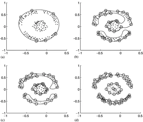
Fig. 1. Clustering of a data set containing 183 points using SVC with C =1. Support vectors are designated by small circles, and cluster assignments are represented by different gray scales of the data points. (a) q=1, (b) q=20, (c) q=24, (d) q=48.
where
Aij =
{
1, i= 1
−2K(Xi, Xj), i̸= 1
, Bi=
{
1, i= 1 0, i̸= 1
At each point X, we define the distance of its image in feature space from the center of sphere as
R2(X) =∥ϕ(X)−a∥2. (7)
In view of quadratic equation and the definition of the kernel [14], the following is got
R2(X) = 1−2∑
j
βjK(Xj, X) (8)
+∑
i
∑
j
βiβjK(Xi, Xj).
The radius of the sphere is R = {R(xj)}, xj is support
vector. The contours enclosed the points in data space are defined by the set{x|R(x) =R}.
B. Cluster Analysis
The number of outlier points are controlled by the pa-rameter C. We have NBSV < 1/C , where NBSV is the
number of Bounded Support Vectors (BSVs) or outliers. As 1/(CN) is an upper bound on the fraction of BSVs, thus 1/(CN) ∈ (0,1]. The value of the parameter C is related to the number of the data points and the willing, how much we want to avoid the outliers. Theqof theK(x, y)is width parameter of Gaussian kernel function. q and C influences the tightness and number of clusters and also the outlier points.
Fig.(1) shows an example of data points clustering with different qs without BSVs (C = 1). The contour of cluster is blur while qincreases, and is fine whileq decreases, but it makes the contour of the cluster affix mutually or break up ifqis over-small or over-large. In Fig.(2a)without BSVs, contour separation does not occur for the two outer rings for any value ofq. When some BSVs are present, the clusters are separated easily Fig.(2b). So the two parametersq and
Fig. 2. Clustering with and without BSVs. The inner cluster is composed of 50 points generated from a Gaussian distribution. The two concentric rings contain 150/300 points, generated from a uniform angular distribution and radial Gaussian distribution. (a) The rings cannot be distinguished when C =1.0 Shown here is q=3.5, the lowest q value that leads to separation of the inner cluster. (b) Outliers allow easy clustering. The parameters are p=0.3 and q=1.0.
IV. STREAM CLUSTERING
A. Stream processing
We consider the problem of clustering a data stream in the sliding window model [16]. The idea behind sliding window is to perform detailed analysis over the most recent data items and over summarized versions of the old ones. Consider n data points Xi1...Xin of a d-dimensional data
space with time stamps Ti1...Tin, the Sliding window (Wi),
contains the last n income data points Xi1...Xin, the new
one overwrites on the oldest one (greatest time stamp) in the array memory of data points [17].
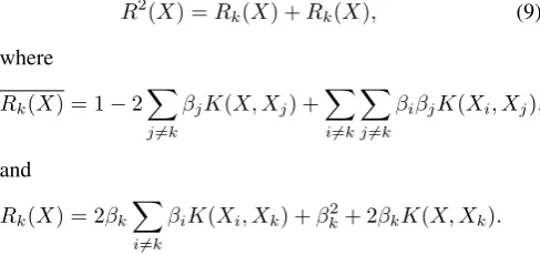
1) Updatingβs: For each pointXwe can write the Eq.(8) as below
R2(X) =Rk(X) +Rk(X), (9)
where
Rk(X) = 1−2
∑
j̸=k
βjK(X, Xj) +
∑
i̸=k
∑
j̸=k
βiβjK(Xi, Xj),
and
Rk(X) = 2βk
∑
i̸=k
βiK(Xi, Xk) +βk2+ 2βkK(X, Xk).
Consider the slide window W at time t0, the points
Xi1...Xin, are clustered by SVC method as Fig.(2) with β1..βn obtained by Eq.(6). If the oldest point Xk is
over-written by a new pointXk′ atkthlocation in memory array
of data points, then for data pointsX(i+1)1...X(i+1)n inW
′ we have
R′2(X) =R′k(X) +R′k(X). (10)
where
R′k(X) = 1−2∑
j̸=k
βj′K(X, Xj) +
∑
i̸=k
∑
i̸=k
βi′βj′K(Xi, Xj),
and
R′k(X) = 2βk′ ∑
i̸=k
βi′K(Xi, Xk′) + (βk′)
2+ 2β′
kK(X, Xk′).
Remark 1: If n be an enough large number, β′k can be obtained as follows
βk′ =λβk′ + (1−λ)βz, (11)
where
βk′ =C∥X ′
k−az∥2
∥v∗−a∗∥2 .
v∗ is a SV point in cluster ∗, with central point a∗, az
is the nearest cluster center point and βz is the lagrangian
coefficient of nearest point toXk′.
β′is the updated value ofβcaused byXk→Xk′ asW→W′.
If the recent change, causes|P| changes in set βjs and |p|
changes in setR2(X
j)s,j=1..n, then we can define the sets
P ={j|βj ≠ βj′} andp={j|R2(Xj)≠ R2(Xj)}.
Lemma 1: All βj′s, j ∈ P can be obtained in O(|P|3), solving a linear system of form
β|P|×1= [A]−|P1|×|P|B|P|×1, β = [βj′∈P]
T. (12)
where
Ai,j= 2(β′kK(Xk′, Xj)−K(Xi, Xj)), i∈p. (13)
Proof:We haven− |p|values of∆R2(Xj) = 0, where
∆R2(X) =R′2(X)−R2(X). Using Eqs.(9, 10, 11), we can expand it as follows
∆R2(X) =−2∑
j∈P
(βj′ −βj)K(X, Xj) (14)
+(βk′)2−(βk)2+ 2(β′kK(Xk′, X)−βkK(Xk, X))
+2βk′ ∑
j∈P
(βj′K(Xj, Xk′)−βjK(Xj, Xk))
+2βk
∑
j∈P−{k}
βj(K(Xj, Xk′)−K(Xj, Xk)).
Using|P|of ∆R2(X)s from set pand factoring the coeffi-cients related toβ′s, we obtain the matrixAandBof linear system (12) and Eq.(13).
Remark 2: To obtain|P|equations for linear system (12) we must have:|P|,|p|< n/2.
As the matrixAis not symmetric, obtainingA−1 is of order
O(|P|3)[18].
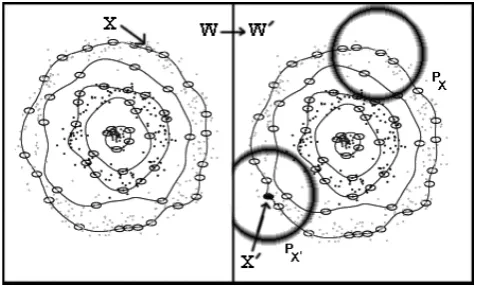
Here, the critical issue is choosing an appropriate set P. Fig.(3) shows an example. As can be seen in the figure, the setP is composed by union of two sets,PX (the circle with
X as cental point) and PX′ (the circle with X′ as cental
point). The updates are only happening around the deleted and added points, thus, we use the points in the two circles as setsPX andPX′. Setting a prefixed radius the circles can
be obtained simply and finally the setP =PX∪PX′.
2) Labeling piece: As mentioned before, labeling piece is a bottleneck in SVC. Ping et al. [8] introduced iSVC a novel approach, whose idea is to cluster the SVs firstly, then construct a classifier based on labeled SVs, finally label other data using the classifier. This algorithm is named as
SAin some books. The steps are as follows
1)Create affinity matrixH with respect to SVs whereH is aV×V matrix withHi,j=K(vi, vj).vi andvj are SVs. 2) Normalize H, using cholesky decomposition [19], into
Hc=D−1/2HD−1/2 , withDii=
∑
[image:3.595.47.291.467.582.2]Fig. 3. As X→X′, W→W′, the data set is changed (including the neighbors ofXandX′), consequently the shape of the related clusters.
3) Find S1..Sκ, the κ largest eigenvectors (κ is specified
by the number of eigenvalues that are larger than 1 [20]) and form Matrix SV×κ = [S1V×1...SκV×1] then normalize
it: Si,j=Si,j2 /(
∑
jSi,j)
1/2.
4) Treating each row of S as a point in Rκ and cluster it into κclusters (using k-means [10]).
5) Labelvi as theithrow’s cluster membership. 6) Label other data in terms of its nearest SV’s label.
Fig.(3) shows the changes of points position, with respect to previous clusters asW→W′.
Consider the setδ={vi′|i∈P∧vi′ is SV}. For data setP, we assume the matrix Hδ
i,j=K(v′i, vj′) with v′i, v′j ∈ δ and
apply above algorithm on it. After 6th step, we have parted
the datasetP, into its clusters.
Lemma 2: ClusterζPX′ inP is a new clusterζ′ inW′ if
and only if
∀ζ in W :ζ∩ζPX′ =∅.
whereζs are the clusters of W andζPX′ is a cluster in set PX′.
Proof: Fig(4.a) shows a data set which contains one cluster and some outlier points. As X→X′ we update the
βs, then some new points are adding to SVs in the set P
(the point in black circles are SVs). Applying SAalgorithm on the Set PX′, two clusters are obtained (ζ
PX′
1 ,ζ
PX′
2 ). As can be seen in Fig(4.b), One of these clusters (ζ1PX′) has no common point with the clusters inW, so it is assigned as new cluster inW′. In order to proof this lemma, this observation can be applied: Suppose the clusterζ1PX′ can not be a new cluster in W′, so it is either a part of cluster ζ in W or a mistaken output ofSAalgorithm. Trusting theSAalgorithm, as the points in ζ1PX′ are outlier in W, clearly it is a new cluster inW′.
Lemma 3: Cluster ζP
X′ in PX′, unions with cluster ζ in W and resize it, and lead it to clusterζ′ inW′ if and only if
(ζ∩ζPX′ ̸=∅)∧(∀ζ in W :ζ∩ζP =∅),
whereζ are the clusters ofW exceptζ.
Proof:In Fig(5.b), setPPX′contains one clusterζPX′.
The same reasoning of previous lemma can be applied to proof. Because of ζPX′ ∩ζ = ∅ the cluster ζ′ can not be
[image:4.595.50.290.52.195.2]joined with ζ.
[image:4.595.305.549.213.334.2]Fig. 4. AsX →X′,W →W′, the data set is changed, addingX′, some outlier points inW are now a new cluster inW′.
Fig. 5. AsX→X′,W→W′, some reshaping in clusters are acquired in the clusterζ.
Lemma 4: Cluster ζ in W, splits into clusters ζ1′...ζS′ in
W′, if and only if there beSclustersζPX
1 ...ζ
PX
S inPX, such
that
(ζ∩ζPX
1 ̸=∅)∧...∧(ζ∩ζ
PX
S ̸=∅).
Proof: Fig(6.a) shows one cluster ζ in W. As can be seen in Fig.(6.b) the setPX parts into two clustersζ1PX and
ζPX
2 . By same observation of previous lemmas, the cluster is splitting inW′ environment.
Lemma 5: Clusters ζ1...ζM in W, merge into cluster ζ′
inW′, if and only if there be one clusterζPX′ inP
X′, such
that
(ζPX′ ∩ζ
1̸=∅)∧...∧(ζPX′ ∩ζM ̸=∅).
Proof: Fig(7.a) shows two clusters ζ1 and ζ2. Adding
X′, setPX′(As can be seen in Fig(7.b)) contains one cluster,
thus the two clusters are merged. Same as previous lemmas this observation can be applied: If the Clusters ζ1 and ζ2, are not merged by adding the new pointX′, then set PX′,
[image:4.595.306.548.644.766.2]can not be contains one cluster. If so, the Algorithm would
Fig. 7. AsX→X′,W→W′, two clustersζ1andζ2 are merged and
composed on cluster.
be outputted a wrong cluster. Although the whole given proofs for the lemmas were intuitive, As the lemmas and the illustrations in examples are very clear, it is no needed for more details and more mathematical definitions.
B. StreamSVC Algorithm
The algorithm of StreamSVC method for a data set N, containing ndata points ofd-dimensional is as follows
(1) using SVC, for sliding windowW, label the clusters as
ζ1...ζκ;
(2) as X→X′, for new sliding windowW′:
(2 - 1) obtain theβ′ for X’, using Eq.(11);
(2 - 2) compose the setsP andp(IV-A1, IV-A1);
(2 - 3) updateβs for setP using lem.(1);
(2 - 4) updateζ1...ζκ toζ1′...ζκ′′:
(2 - 4 - 1)delete the clusters which has no BSVs;
(2 - 4 - 2)compose the new clusters using lem.(2);
(2 - 4 - 3)resize the clusters using lem.(3);
(2 - 4 - 4)split the clusters using lem.(4);
(2 - 4 - 5)merge the clusters using lem.(5);
(3) if the stream is not ending, goto step(2);
The most important issue to increase the algorithm’s accuracy is to compose the sets P and p (Step 2 - 2). Because of the time complexity order of (Step 2 - 3), to achieve overall complexity of O(n), we must choose |P| = √3n. The appropriate points in set P and p, are
the points, such that the points in p have relatively far distance from X and X′. We can suggest variant ways to achieve a good P and p. In the previous examples, simply a radius is prefixed and P is composed by union of PX
andPX′ (see Fig.(3)). For the setp, we can simply choose
p =P. Introducing the other ways to obtain P and p, we can observe following algorithm. Wang et al. [7] obtains a similarity matrix as follows: A link is created between a pair of points, r and s, if and only if r and s have each other in the list of their k1nearest neighbors, wherek1 is a user pre–specified parameter. The strength of a link between two points is expressed by the number of nearest neighbors that are shared by the two points, their similarity is defined as
sim(r, s) =|N N(r)∩N N(s)|,
where N N(r) and N N(s) are the nearest neighbor list of
r and s, respectively. Based on that we can introduce an
TABLE I
THE EXPERIMENTAL RESULTS OF IRIS DATA SET IN STREAM FORM. THE INITIAL PARAMETERS FORSVCAREq= 4.2,C= 0.03AND FOR
OBTAININGβ′kFROMEQ.(11),λ=0.5
Time 0.1 0.2 0.3 0.5 0.7 0.8 0.9 No. Clusters 3 3 3 3 3 3 3
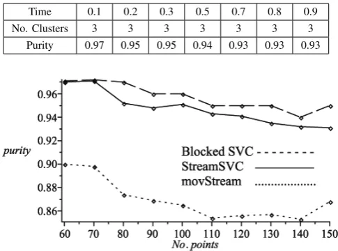
[image:5.595.307.550.98.278.2]Purity 0.97 0.95 0.95 0.94 0.93 0.93 0.93
Fig. 8. Experimental results of iris data set based on purity, from 3 different methods. The Blocked SVC, StreamSVC, movStream with|W|= 60
algorithm as follows: obtaining the similarity matrix, we choose|P|the number of points nearX andX′, the number of ones which have a strength similarity (sim(X, Xi))> α),
whereαis a prefix number and composes setPα.
Now choosing setpis quit simple. We just want the points in
pwhich have relatively far distance fromX andX′, simply we can choosep=Pα.
V. EXPERIMENTALRESULTS
This section evaluates the performance of our algorithm. The following experiments are conducted on Microsoft Windows XP Home Edition, with 1GB main memory and 2.4GHz CPU. The algorithm is tested with two different data sets. First one is iris data set [21] in stream form. The data set contains three clusters, and total 150 points (50 points for each cluster). We initialize the first sliding window by 60 points, 20 points from each cluster, then after each 0.01 second, periodically, a single point from each cluster is added.
Table I showspurityin timeline. Purity is average percentage of the dominant class label in each cluster [1]. In Fig.(7) the results are compared with movStream [12] (with MaxNum-Cluster=3 and MinNumCluster=2) and Blocked SVC with initial values of q and C, same as Table I. Blocked SVC, reapplies the original SVC after every 10 points change. Because of the order of SVC, it cannot be an appropriating method for streams, but as it is good reference to examine the accuracy of StreamSVC, Thus, we compared it with our method. In this experience we choose setP as union ofPX
andPX′, wherePX is the set of point in a circle withX as
central point and radius=1.
TABLE II
THE NUMBER OF EACH CASE IN THE PROBED SLIDING WINDOW.
W 10,001-11,000 80,001-81,000 100001-101000 210001-211000 310,030-311,029 sumrf 1000 0 0 345 0 snmpget 0 0 109 0 396
gsspass 0 8 10 0 0 nmap 0 0 1 0 0 portswp 0 0 12 0 0 satan 0 753 0 0 0 warezm 0 12 33 0 0
Fig. 9. Experimental results of KDD-CUP-99-corrected with Blocked SVC and SVC with the sameCandq. For StreamSVCλ=0.65.
type. To examine the StreamSVC, we used a subset of whole data set named KDD-CUP-99-corrected. The dataset contains 311029 data points, and 42 dimensions. As in OCallaghan et al. (2002) and Aggarwal et al. (2003), all 34 continuous attributes will be used for clustering. We initialized the parameters as follows:|W|=1000,q=2.1,C=1 and the setP
as union of two setsPX andPX′, where setPX contains the
5 nearest point toX, so|P|=10. The initial sliding window, contains two kinds of attacks (186 cases of smurf and 103 cases of snmpgetattack) and the normal connections (711 cases), while from data point 210001 to 211000 we have 345 cases of smurf and 655 cases of normal connections. Table V, shows the number of each case in the probed W. Fig.(9) shows the purity of the clusters in the process and compared it with Blocked SVC. The result shows more than 93% accuracy for the method, and in the most areas, the deviation of its curve relatively to Blocked SVC’s curve, is averagely 5-6%. The results shows that, the accuracy of the algorithm, is mostly equals to the original SVC algorithm for non–stream data sets. As we choose P=10, then total time is highly reduced, while the accuracy is still acceptable.
VI. CONCLUSION
In this paper we introduced StreamSVC, a novel algorithm to cluster high-dimensional data streams based on SVC method. StreamSVC applied SVC, to initialize the first clusters, then based on the changes in data environment, it takes a subsets of the dataset which are affected by the change, and reobtains the SVC’s parameters to updates the clusters. The most critical part is preparing a good subset of the dataset which the complementary of it contains only the parts of dataset which surely are not changed in any of their parameters.
In the experimental result section, some real data sets are applied. The first one was the famous iris data set. As iris data set is a standard benchmark in the pattern recognition
literature, we applied it in stream formatting. The reason was to assay the accuracy of the algorithm, and the second data set, KDD-CUP-99, to test both time efficiency and accuracy of clusters.
The experimental results shows high accuracy and time effi-ciently of the presented method. As the strength of original SVC is guaranteed, for every data sets, the accuracy and time complexity order can be acceptable.
ACKNOWLEDGMENT
With special thanks to Dr. L. Sharif and Prof. S. Kazem who helped the authors to execute the ideas and were great guiders through writing this paper.
REFERENCES
[1] J. Han and M. Kamber, Data Mining: Concepts and Techniques, 2nd ed. San Francisco: Morgan Kaufmann, 2006, ch. 7, pp. 308–466. [2] L. O’Callaghan, N. Mishra, S. G. A. Meyerson, and R. Motwani, “Streaming-data algorithms for high-quality clustering,”ICDE Con-ference, 2002.
[3] C. Aggarwal, J. Han, J. Wang, and P. Yu, “A framework for clus-tering evolving data streams,” inIn Proceedings of the International Conference on Very Large Data Bases (VLDB), 2003, pp. 81–92. [4] D. Abadi, D. Carney, U. Cetintemel, M. Cherniack, C. Convey, S. Lee,
M. Stonebraker, N. Tatbul, and S. Zdonik, “Aurora: a new model and architecture for data stream management,” VLDB Journal, vol. 12, no. 2, pp. 120–139, 2003.
[5] C. Aggarwal,Data Streams: Models and Algorithms. New York: Springer, 2007.
[6] A. BenHur, D. Horn, H. Siegelmann, and V. Vapnik, “Support vector clustering,”Machine Learning Research, vol. 2, pp. 125–137, 2001. [7] J.-S. Wang and J.-C. Chiang, “An efficient data preprocessing
proce-dure for support vector clustering,” Journal of Universal Computer Science, vol. 15, no. 4, pp. 705–721, 2009.
[8] L. Ping, Z. Chun-Guang, and Z. Xu, “Improved support vector clustering,”Engineering Applications of Artificial Intelligence, vol. 23, pp. 552–559, 2010.
[9] J. Lee and D. Lee, “An improved cluster labeling method for support vector clustering,” inTransactions on Pattern Analysis and Machine Intelligence, ser. 3, vol. 27, 2005, pp. 461–464.
[10] R. Dua and P. Hart,Pattern Classification and Scene Analysis. J. Wiley and Sons, 1973.
[11] C. C. Aggarwal, J. Han, J. Wang, and P. S. Yu, “On high dimensional projected clustering of data streams,” Data Mining and Knowledge Discovery, vol. 10, no. 3, pp. 251–273, 2005.
[12] L. Tang, C. J. Tang, L. Duan, C. Li, Y. X. Jiang, C. Q. Zeng, and J. Zhu, “Movstream: An efficient algorithm for monitoring clusters evolving in data streams,” in2008 IEEE International Conference on Granular Computing, GRC, 2008, pp. 582–587.
[13] D. Horn, “Clustering via hilbert space,”Physica A, vol. 302, pp. 70– 79, 2001.
[14] D. Horn, A. BenHur, H. Siegelmann, and V. Vapnik, “A support vector method for clustering,” in Advances in Neural Information ProcessingSystems, ser. Proceedings of the 2000 Conference, T. Leen, T. Dietterich, and V. Tresp, Eds., vol. 13. MIT Press, 2001, pp. 367–373.
[15] R. Fletcher,Practical Methods of Optimization. Chichester: Wiley-Interscience, 1987.
[16] E. Ikonomovska, S. Loskovska, and D. Gjorgjevik, “A survey of stream data mining,” inProceedings of 8th National Conference with International Participation, ETAI, 2007, pp. 19–21.
[17] C. Aggarwal, H. J. wei, W. Jian-yong, and Y. P. S, “A framework for projected clustering of high dimensional data streams,” inProceedings of the 30th International Conference on Very Large Data Bases, Toronto, Canada, 2004, pp. 852–863.
[18] K. S. Miller, “On the inverse of the sum of matrices,” vol. 54, no. 2, pp. 67–72, 1981.
[19] M. Abramowitz and I. A. Stegun,Handbook of Mathematical Func-tions. New York: Dover Publications, 1972.
[20] T. Zheng, L. Xiaobin, and J. Yanwei, “Disturbing analysis on spectrum clustering,”Science in China(SeriesE), vol. 37, no. 4, pp. 527–543, 2007.
[21] R. Fisher, “The use of multiple measurments in taxonomic problems,”