Docking a UAV using a robotic arm and computer vision

and Computer Vision

J.H. (Jort) Baarsma

MSc Report

Committee:

Prof.dr.ir. S. Stramigioli

Dr.ir. F. van der Heijden

Dr.ir. M. Fumagalli

Dr.ir. R.G.K.M. Aarts

March 2015

Summary

The aim of this Thesis is to research the possibility of docking an airborne UAV using a robotic arm and computer vision. In the scope of the SHERPA project on robot collaboration in Alpine rescue scenario‘s a robust and autonomous way of retrieving small scale UAV‘s is required. In a scenario where landing the UAV on a mobile ground station is not possible and landing on the ground could be harmful to the drone, docking the UAV while it is airborne using a robotic arm would be the best solution.

Contents

1 Introduction 1

1.1 Context . . . 1

1.1.1 Alpine search and rescue . . . 1

1.2 Problem statement . . . 3

1.3 Prior work . . . 3

2 Analysis & Design 5 2.1 System introduction . . . 5

2.1.1 Subsystem allocation . . . 5

2.1.2 Definitions and notation . . . 5

2.2 Setpoint generator-subsystem . . . 7

2.2.1 Strategies . . . 7

2.2.2 Follow distance . . . 8

2.2.3 Path generator . . . 8

2.3 Robotic arm-subsystem . . . 10

2.3.1 Kinematic chain . . . 10

2.4 UAV-subsystem . . . 12

2.4.1 Quadcopter . . . 12

2.4.2 IMU . . . 13

2.5 Computer vision-subsystem . . . 14

2.5.1 Feature extraction . . . 14

2.5.2 Marker design . . . 14

2.5.3 Pose estimation . . . 17

2.6 State estimator-subsystem . . . 22

2.6.1 Transformations . . . 22

2.6.2 Kalman filter . . . 23

2.6.3 Extended Kalman filter . . . 24

2.6.4 Extended Kalman filter design . . . 25

3 Implementation and Realisation 27 3.1 Software Implementation : ROS . . . 27

3.1.1 Brain node . . . 29

3.1.2 Robot controller : FRI node . . . 31

3.1.3 Data acquisition : DUAVRACV Logger . . . 33

3.2 Hardware realisation . . . 34

3.2.3 Drone substitute : Xsens IMU . . . 38

3.2.4 Camera . . . 39

4 Results 41 4.1 Measurements . . . 41

4.1.1 Validation . . . 41

4.1.2 Reproducibility . . . 41

4.2 Experiments with Xsense IMU drone substitute . . . 42

4.2.1 General behavior impressions . . . 42

4.2.2 Movement in Y with occlusion . . . 42

4.3 Experiments with Parrot AR.Drone . . . 45

4.3.1 Computational load . . . 45

4.3.2 Qualitative results . . . 45

5 Conclusions & recommendations 47 5.1 Conclusions . . . 47

5.2 Recommendations . . . 47

1 Introduction

1.1 Context

1.1.1 Alpine search and rescue

Introducing robotic platforms in a rescue system is envisioned as a promising solution for sav-ing human lives after an avalanche accident in alpine environments. With the popularity of winter tourism, the winter recreation activities has been increased rapidly. As a consequence, the number of avalanche accidents is significantly raised. According to the statistics provided by the Club Alpino Italiano, in 2010 about 6,000 persons were rescued in alpine accidents in Italy with more than 450 fatalities and about thirty thousand rescuers involved, and with a wor-rying increasing trend of those numbers. In 2010 the Swiss Air Rescue alone conducted more than ten thousand missions by helicopters in Switzerland with more than 2,200 people that were recovered in the mountains [1].

To this aim, a European project named “Smart collaboration between Humans and ground-aErial Robots for imProving rescuing activities in Alpine environments (SHERPA)” has been launched.

SHERPA

The activities of SHERPA are focused on a combined aerial and ground robotic platform suit-able to support human operators in accomplishing surveillance and rescuing tasks in un-friendly and often hostile environments, like the alpine rescuing scenario specifically targeted by the project.

What makes the project potentially very rich from a scientific viewpoint is the heterogeneity and the capabilities to be owned by the different actors of the SHERPA system: the “human” rescuer is the “busy genius”, working in team with the ground vehicle, as the “intelligent don-key”, and with the aerial platforms, i.e. the “trained wasps” and “patrolling hawks”. Indeed, the research activity focuses on how the “busy genius” and the “SHERPA animals” interact and collaborate with each other, with their own features and capabilities, toward the achievement of a common goal.

Trained wasps The “Trained wasps” are small rotary-wing unmanned aerial vehicles (UAVs), equipped with small cameras and other sensors/receivers and used to support the rescuing and surveillance activity by enlarging the patrolled area with respect to the area potentially “covered” by the single rescuer, both in terms of visual information and monitoring of emer-gency signals. Such vehicles are technically designed to operate with a high degree of autonomy and to be supervised by the human in a natural and simple way, like they were “flying eyes” of the rescuer, helping him to comb the neighbouring area. UAVs are specifically designed to be safe and operable in the vicinity of human beings. As a consequence they have a limited oper-ative radius.

of the small scale UAVs and the equipment storage element, are mechanically conceived to be confined in the so called “SHERPA box”.

Patrolling hawks The “patrolling hawks” are Long endurance, altitude and high-payload aerial vehicles, with complementary features with respect to the small-scale UAVs introduced before, complete the SHERPA team. Within the team, they are used for construct-ing a 3D map of the rescuconstruct-ing area, as communication hub between the platforms in presence of critical terrain morphologies, for patrolling large areas not necessarily confined in the neigh-borhood of the rescuer, and, if needed, to carry the “SHERPA box” in places non accessible to the rover. They fly at a height of around 50-100 m above ground (or trees).

1.2 Problem statement

In a system where robots collaborate to assist rescue operations small scales multi-rotor UAV‘s need to be able to autonomously return to a ground rover where they can be recharged and stores. A multifunctional robotic arm on the ground rover can be used to dock the UAV and re-turn it to the recharge station inside of the “SHERPA box”. The Conceived scenario‘s for docking the UAV were:

• The multirotor lands on a helipad on top of the rover and is then docked by the robotic arm.

• The multirotor lands or falls on the ground near the rover and is then docked by the robotic arm.

• The multirotor is docked while flying in close proximity to the rover.

The first scenario would be the ideal scenario whenever possible but this is not possible in all weather conditions or when the rover is angled at a slope. In the second scenario the type of surface which is chosen is important, if a flat surface without any foliage or rocks can be found this is a good alternative. However this scenario is also not robust when the surrounding area is rocky or covered with foliage where the drone could be damaged or lost when attempting to land. The last scenario would be the most challenging to realize but would best for the longevity of the drone when executed reliably, and will be the focus of this research.

In this scenario the drone can theoretically be docked in any situation where the drone can approach the rover. The key piece of information in this problem is relative position and move-ment of the drone with respect to the rover. The GPS signals of the rover and UAV are only up to a few meters and can only get the vehicles in close proximity of each other. From this distance the drone can be found using a camera mounted on the robotic arm and followed by estimating the pose of the drone. The sensors inside the drone can assist the estimate when the pose cannot be estimated. Following the drone is a virtual servo-ing “Camera in hand” prob-lem and docking the drone is an extension to that probprob-lem by decreasing the follow distance until docking can be performed.

To summarize the problem statement in one sentence: Is it possible to follow and dock a multi-rotor UAV using a robotic arm and computer vision?

1.3 Prior work

2 Analysis & Design

In this chapter the system to follow and dock the drone is explained.

2.1 System introduction

The system used to follow and dock the UAV is using visual pose estimation system in combin-ation with IMU measurements from the UAV.

To be able to dock the UAV using a robotic arm the pose estimate of the UAV needs to be pre-cise. The best way to achieve this is to measure the pose itself by means of some sort of pose estimation. In this system the method of pose estimation is done by means of computer vision. To improve the pose estimation additional sensors can collaborate to support the weak features of the vision sensor. In this system it was chosen to use the IMU data, of the target UAV that is to be docked, as an additional sensor and fuse the measurements with a state estimator.

2.1.1 Subsystem allocation

For clarity the system has been divided into subsystem which will be discussed in detail in their respective sections. The subsystems that are envisioned are:

• Robotic Arm subsystem

• Setpoint generator subsystem

• State estimator subsystem

• Computer vision subsystem

• UAV subsystem

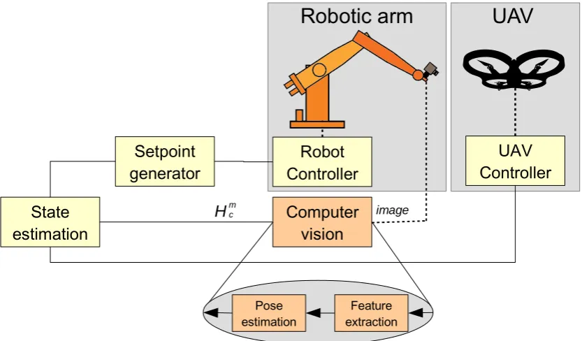
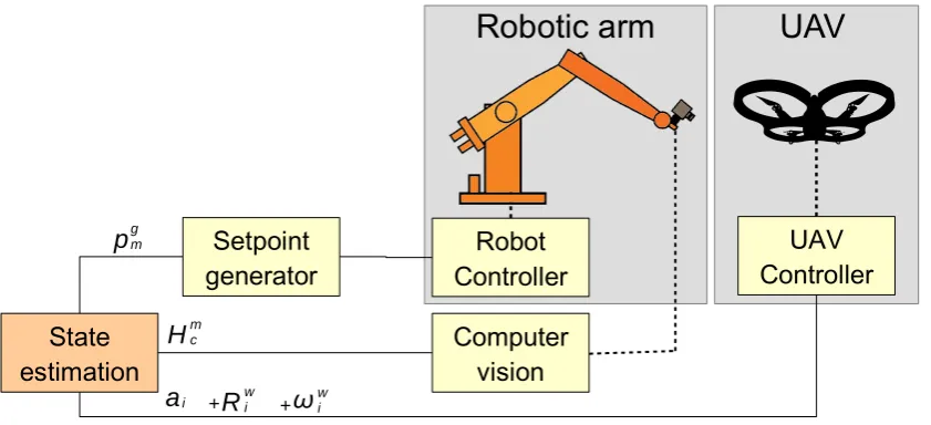
The connection between the system is shown in figure 2.1. The computer visions pose estim-ationHmc is combined with the acceleration~aii, orientation~qiw and angular velocity~!wi of the

UAV into the state estimator which produces an optimal state estimate of the UAV position~p§g_i based on the known information. From this optimal estimate of the drone location a setpoint is derived which followed by the controller of the robotic arm.

2.1.2 Definitions and notation

This section define some variables and notations which hold throughout all the subsystem of the system.

In this report Vectors~vwill be indicated be by small letters with a harpoon and matricesAwill be a capitol boldface letters. The notation for a estimate is a tilde above the symbol ˜a and an optimal estimate is denoted with a asterisk above the symbola§.

Relative poses are described by homogeneous matricesHab2R4£4where theadefines the

des-tination frame andb describes the reference frame. A alphabetic characters in superscript notation for a variable for will indicate the reference frame in which that variable is viewed. A homogeneous matrix is composed of a rotation matrixRba and translation vector~tab and is a

powerful method of describing kinematic chains.

H_ab= "

Rb a ~tab

~₀T ₁

Setpoint

generator

Computer

vision

State

estimation

Robot

Controller

UAV

Controller

p

m H

g s

+

H

R

a

image

Robotic arm

UAV

+

ω

Figure 2.1:Schematic representation of the setup.

H world

H base

H hand

H camera

H marker H _imu

= Hglobal

Figure 2.2:Frames in the method

The system and its subsystems have several frames which are referred to throughout the report by only their letter, these are listed in table 2.1 and illustrated in figure 2.2. The global reference frame is not alligned with the world coordinate frame due to the unknown orientation with respect to magnetic north.

Letter Frame description

g The base of the robotic arm b The base of the robotic arm i The IMU of the UAV.

w Defined by magnetic north and gravitational vector h End-effector of the robotic arm

c Camera frame mounted on end-effector. m Marker frame that is mounted on the UAV

s Setpoint frame

Setpoint

generator

Computer

vision

State

estimation

Robot

Controller

UAV

Controller

p

m H

g s

Robotic arm

UAV

Figure 2.3:Control schema - Set-point generator.

2.2 Setpoint generator-subsystem

The set-point generator sub-system is responsible of generating set-points for end-effector of the robotic arm to follow. The generated setpoint is based on the optimal estimate of the UAV position and a strategy the generator is set to. These strategies are determined beforehand based on likely scenarios and what strategy is used is determined by the system with input from the user. There is also a safety layer in this subsystem which limits the (angular) velocity of the moving set-point and keeps the robot inside of its work envelop.

The subsystem is located in the system as shown in figure 2.3. The input of the system is:

• The optimal estimate of the position of the marker with respect to the robotic arm base

§

Hmg.

The output of the system is:

• The a desired pose set-point for the robotic arm controllerH_hg.

2.2.1 Strategies

The strategies that are used are based on the distance of the drone to the work envelop of the robot and the desired behavior specified by the user. The selection of strategy and transition between strategies is done by the system itself but the user has control over what strategies are allowed. The user can force idle mode or (dis)allow any state to get the desired behavior. The strategies names are influenced by hunting behavior and most strategies focus on following the marker at a distance_d~_{. The set-point generator strategies are:}

• Idle: This is the resting position in which the system does not do anything. The set-point is an exact copy of the current pose and the strategy only changes when the user requires it.

• Spot: In this strategy the set-point is set to a fixed point from where the camera can see the scene. When the marker is found the strategy transitions into the “Watch” strategy.

• Watch: If the marker is found but too far away to follow at a fixed distance_d~_{st akl it is}

Follow z camera

Follow x global

Follow -z marker

Figure 2.4:Follow distance illustration

• Stalk: In this strategy the marker pose is followed at a fixed distance_d~_{st alk. If the}

set-point goes outside of the work envelop the the strategy transitions back into the “Watch” strategy. If the marker can also be followed at a close distance_d~_{pr e y the strategy}

trans-itions into the “Prey” strategy.

• Prey: In this strategy the marker is followed at a close distance of_d~_{pr e y. The distance} ~

dpr e y is the closest distance to which the vision system can reliably estimate the pose of

the marker and is used as a buildup to docking the drone. Keeping the marker in view of the camera when the drone is moving at this distance can be challanging. If the setpoint goes outside of the work envelop the the strategy transitions back into the “Stalk” strategy. If the marker is so close that it can be docked the strategy transitions into the “Catch” strategy.

• Catch: In this strategy the last known marker pose is saved and the controller quickly ap-proaches this marker disregarding new measurement. This is because the vision meas-urement is assumed to be not reliable at distances closes than 20cm.

When the pose is lost for long enough the strategy transitions back into the “Spot” strategy for any of the strategies in which the pose estimate is used.

2.2.2 Follow distance

The reference frame of the follow distance _d~_{was deliberately kept ambiguous in reference}

frame in the discussing on generator strategy. The system can either follow the marker a fixed distance in the frame of the marker_d~m_{, in the camera framed~}c _{or in the global framed~}g _as

illustrated in figure 2.4. All three methods center the marker on the image plane but have dif-ferent results as end-effector pose. Following of the drone with respect to the minus Z axis of the marker is the most logical method of following but has the disadvantage of amplifying any rotational errors due to the fact they are multiplied by the follow distance_d~_{. Following with}

respect to the marker will be implemented for docking because this allows for the best align-ment but assuming that the drone is more or less parallel to the ground during the following and docking the method of following in the global frame was preferred for all other scenarios.

2.2.3 Path generator

If the set-point and current robot end-effector are far away from each other the robot cannot follow and dangerous scenarios can occur. For this reason a path planner is used that calculates intermediate set-points between the current pose and the desired pose with a limited velocity for every step. This velocity limiting is achieved by means of a logarithmic map and applying a limit on the resulting twist. The path and twist is updated every time there is a new set-point. The desired pose for the end-effectorHsg can be written as a combination of the current

Hsg=H_hgHsh

The exponential map is used which describes the resulting pose when a constant twist is ap-plied fort time. The set-point is used as the end-point and the end-effector is subject to a constant twist in body fixed frame.

Hsg=Hhg(t)=H g h(0)e

˜

T_hh,gt

In this equation the time dependanceH_hg(t) is shown for clarity, all other mentions ofH_hg will be at time instance 0. This reworked to find the twist of the end-effector with respect to the base in its body fixed frame.

˜

T_hh,g=1_tlog≥HghHsg

¥

=Kplog

≥ Hsh

¥

In which ˜T is a skew symmetric matrix of the Twist vector ~_{T and the logarithm is a matrix}

logarithm. What eqation 2.2.3 represents is the required constant twist to get to poseHsg int

time. Because the requirement is to get to the setpoint as fast as possible with a limited twist a the factor1_t is replaced by a gain factorKpand a limiter is put on the Twist.

if _||T~_{|| >Tmax then : T}~₌

(

~

T_·Tmax

||~_T||

)

The limiter used scales down the twist when the norm of the twist vector_T~_{becomes higher}

than a set value. Because the twist is only scaled the traveled path will be identical to the path that was not limited.

To calculate the intermediate pose on the pathHpg the matrix exponential is used.

Hpg=H_hgeT˜

Setpoint

generator

Computer

vision

State

estimation

Robot

Controller

UAV

Controller

s

Robotic arm

UAV

Figure 2.5:Control schema - Robotic arm.

2.3 Robotic arm-subsystem

The Robotic arm-subsystem is responsible for controlling the robot towards the desired pose setpoint. This subsystem is required for the communication to the hardware of the robot arm, the robot itself will have the low-level motor controllers.

The subsystem is located in the system as shown in figure 2.5. The input of the system is:

• The a desired pose set-point for the robotic arm controllerH_hg. The output of the system is:

• A connection to the robotic arm.

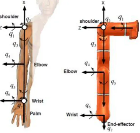
2.3.1 Kinematic chain

Figure 2.6:Kinematic chain

Behavior

The robot follows a set-pointHsg which is near the current robot poseH_hg. The robot is

Setpoint

generator

Computer

vision

State

estimation

Robot

Controller

UAV

Controller

+

R

a

Robotic arm

UAV

+

ω

Figure 2.7:Control schema - UAV.

2.4 UAV-subsystem

The UAV subsystem is responsible making the drone fly and sending IMU measurements to the system. The drone is manually controlled by an operator

• Feature extraction

• Pose estimation

The subsystem is located in the system as shown in figure 2.7.

The input of the system is a network connection coming from the drone. The output of the system is:

• The acceleration measurement from the UAV~ai mu, in body fixed coordinates.

• The orientation measurement from the UAVRwor ld i mu 2.4.1 Quadcopter

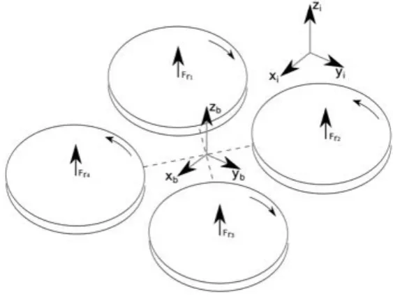
A quadcopter drone is a type of unmanned aerial vehicle using four rotors for its actuation. A simplified quadcopter is shown in Figure 2.8.The four rotors can be seen as inputs and are used to move the quadcopter in six degrees of freedom (three translations and three rotations). The degrees of freedom that can be controlled in a quadcopter are the euler angles roll, pitch, yaw and the movement in body fixed z direction. Because the body of the drone can be rotated with respect to the fixed world the movement in body fixed z direction the drone can also translate in global x and y direction.

The control is done using rotor pairs on opposing sides of the quadcopter that spin in opposite direction. The propellers are made much that all rotors generate a lift upwards but the clock-wise rotating rotors generate a negative moment°Mz and the counter-clockwise rotors a

pos-itive momentMz. These moments counteract when both pairs of rotors are controlled to

Figure 2.8:Quadcopter basics

(body fixed x and y) have almost no stiffness or damping due to being airborne and are thus susceptible to disturbance.

Because the drone is chosen to be an off-the-shelf product and not being controlled by the system no additional analysis information on the drone is required.

2.4.2 IMU

Setpoint

generator

Computer

vision

State

estimation

Robot

Controller

Controller

UAV

H

Feature extraction Pose

estimation

image

Robotic arm

UAV

Figure 2.9:Control schema - Computer vision.

2.5 Computer vision-subsystem

The computer vision subsystem is responsible interpreting coming from the end-effector mounted camera. Specific features are extracted from the images based on color and used as points for pose estimation. The computer vision subsystem itself comprises of these two parts: thefeature extractionandpose estimation.

The subsystem is located in the system as shown in figure 2.9. The input of the system is:

• a digital video stream of image coming from the camera.

The out of the system is:

• A relative pose between the camera and the markerHcamer amar ker. 2.5.1 Feature extraction

2.5.2 Marker design

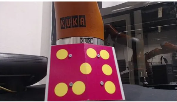
The marker has been designed with two clear goals in mind: A clear vibrant color that is distin-guishable in most scenes and non-planar constellation of image points to avoid pose ambigu-ity. The first requirement is met by using Magenta, a color that is not very common but vibrant when printed on a sticker due to the use of CMYK ink in printers. The second is accomplished by folding the sticker over a bend plate that has an inside angle of 155 degrees. The marker can be seen in figure 2.12.

Color representation

orange color which show an a seemly arbitrary change in R G and B values as shown in figure 2.10.

-31 R

+24 G

+59 B

R 217

G 118

B 33

R 186

G 132

B 92

Figure 2.10:Unintuitive color representation in RGB.

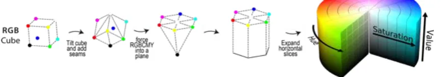
The hue saturation value (HSV) representation was chosen as representation for the image which is more suitable for filtering out a desired color from the image. The HSV representa-tion remaps the RGB colorspace by tilting the cube representarepresenta-tion of RGB on its side with the white value [255,255,255] point to the top and black [0,0,0] to the bottom. The colors red, green, blue, cyan, magenta and yellow are now projected onto a plane and expanded into a cylindrical space. The angle of this cylindrical representation is the hue which represents the color, the ra-dial component is the saturation and the height is the value. The process of going from RGB to HSV is illustrated in figure 2.11.

Figure 2.11:RGB to HSV

Filters

The marker that was designed has a distinct magenta color that is vibrant due to the printing process using CMYK ink. In figure 2.13a an example image from the camera can be seen. Using a threshold operation in the HSV color-space all the magenta regions are selected. As can be seen in figure 2.13b the image contains a large number of small magenta regions due to noise. The image is improved by using a morphological erode operation followed by a morphological dilate operation, this combination of morphological operations is called “opening”. The result-ing image shown in figure 2.13c only shows large magenta regions.

Every magenta region remaining in the image is cut out of the original image into a new image that will be individually processed. For every magenta cutout region a HSV threshold filter is is applied now selecting a yellow color. The resulting image is again enhanced by a morphological “opening” operation and every resulting region is evaluated for it‘s : roundness, height/width ratio and area. Every region that passes the evaluation is labeled as a “dot feature” and if ex-actly eight dot features are found the feature extraction is considered successful and the image processing is stopped. The other magenta regions of interest are not processed if a eight “dot feature” object has been found. If multiple markers are present in the scene, only one will be found.

Figure 2.12:Original image.

(a)HSV filtered image (b)After morphological operations

(c)Cut out magenta region of interest (d)HSV filtering and morphological operations

2.5.3 Pose estimation

If the feature extraction was successfulnpoints are found. To calculate the relative pose of the marker with respect to the camera then point 2D to 3D point correspondence is calculated ,which projects the three dimensional points onto the image plane. The pose estimation start with modeling the 2D to 3D projection which is done using a pinhole camera model.

Pinhole camera

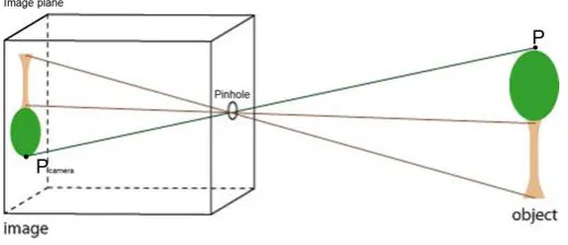
The pinhole camera model was chosen because we are only interested in the centers or the ellipses for pose estimation which are unaffected by the point spread function of the lens. With this basic model three dimensional points can be mapped to a two dimensional image plane by means of matrix multiplication. In the pinhole camera model the pinhole is the origin of the frame ,the image plane is located focal distance f behind the origin and the Z axis is the axis perpendicular to the image plane through the origin. In the pinhole camera model the points on the image plane and in the three dimensional space are described in homogeneous coordinates, making them scale invariant by having one extra dimension. The notation for the image plane points~√₌{u,v,1}T and three dimensional Cartesian points~p₌{x,y,z,1}T is different to avoid confusion.

The point~pwill be mapped to location√~on the image plane which is the intersection point between the line, coming from point~pthrough the origin, and the image plane. The image on the image plane is inverted due to the fact that the projection lines cross at the pinhole. The model is shown in figure 2.14.

Figure 2.14:Pinhole camera model

From this model the following two projective equations can be derived:

u§₌ f x

z v§=

f y

z (2.1)

The asterisk in equation 2.1 is to indicate that the value foruandvis in meters and not pixels. The image sensor has a sensitivity ofmxandmy (pixels/meter) on the sensor surface in X and

Y respectively. The origin of the image is also shifted bycuandcv(in pixels) to be at the edge of

the sensor, which ensure that the range of image indexes is positive.

u₌mxf x

z +cu v=my

f y

z +cv (2.2)

s√~=s 0 B @ u v 1 1 C A= 0 B @

muf 0 mxcu 0

0 mvf mycv 0

0 0 1 0

1 C A 0 B B B B @ X Y Z 1 1 C C C C A= h

K|~₀ip~ (2.3)

The K2R3£3 matrix is called the intrinsic camera matrix and described how 3D points are mapped to a 2D plane when the camera is located at the origin and aligned with the reference frame. This matrix is also sometimes called the “Camera Calibration Matrix” because it is a which is constant when not changing the capture resolution or focus distance. The intrinsic camera matrix is assumed to be known for the camera used.

Camera movement

In the pinhole camera equation 2.3 it is presumed that the coordinates of the marker points

~

p are known in camera coordinates. In the problem of pose estimation this is no longer the case because the camera is transformed by an unknown rotationR_CM and translation~t_MC with respect to the marker frame. The individual marker points are now defined as {~pM

1 ···~pnM} in

the marker reference frame, and the resulting image points as {√~1···√~n}. The projection model

now becomes :

s√~i=K

h

R_CM ~t_CMi~p_iM₌K T_CM~pM_{i =}P~pM_i (2.4)

In this equationP2R3£4 is defined as the projection matrix which can be decomposed into the intrinsic camera matrixK which (explained in 2.5.3) and the extrinsic camera matrixTM

C 2

R3£4. The notation for the extrinsic camera matrix is equal to the homogeneous transform matrixT_CM without the last row, making the matrix scale dependent.

In case of pose estimation the image points~√i, the marker points in the marker framep~_iM and

the intrinsic camera matrixK are known and equation 2.4 needs to be solved for the relative poseTM

C .

DLT : Pose estimation

In the Direct Linear Transform method the 12 parameters of the projection matrixPare estim-ated up to a scalar value.

s~√i=P~pi=

2 6 4

P11 P12 P13 P34

P21 P22 P23 P34

P31 P32 P33 P34

3 7 5~pi

Writing out this matrix into three equations:

P11xi+P12yi+P13zi+P14=s(ui)

P21xi+P22yi+P23zi+P24=s(vi)

P31xi+P32yi+P33zi+P34=s(1)

The third equation can be eliminated to solve the homogeneous scaling factors, yielding the following equations per marker point.

P11xi+P12yi+P13zi+P14°(P31xi+P32yi+P33zi+P34)ui=0

Combining the equations for alln points and placing them into a matrix where the columns represent projection matrix parameters results in [5]:

2 6 6 6 6 6 6 6 4

x1 y1 z1 1 0 0 0 0 °u1x1 °u1y1 °u1z1 °u1

0 0 0 0 x1 y1 z1 1 °v1x1 °v1y1 °v1z1 °v1

..

. ... ... ... ... ... ... ... ... ... ... ...

xn yn zn 1 0 0 0 0 °unxn °unyn °unzn °un

0 0 0 0 xn yn zn 1 °vnxn °vnyn °vnzn °vn

3 7 7 7 7 7 7 7 5 § 2 6 6 6 6 6 6 6 6 6 6 6 6 6 6 6 6 6 6 6 6 6 6 4 P11 P12 P13 P14 P21 P22 P23 P24 P31 P32 P33 P34 3 7 7 7 7 7 7 7 7 7 7 7 7 7 7 7 7 7 7 7 7 7 7 5

=~₀

With at least six points correspondence a estimate for the projection matrix ˜P can be found with singular value decomposition as the Eigen vector corresponding to the lowest singular value. The inverse of the known intrinsic camera matrixK is used to find the extrinsic camera matrix ˜HM

C up to a scalar value.

sT˜_CM=K°1_P˜

Because it is known that the determinant of the rotation matrix should equal one the scaling factorscan be found by:

s=_det(R1 ₎

The DLT method gives a good initial estimate of the pose but is susceptible to noise [5] which is likely to be present in the signal. The DLT method is used to get a rough estimation of the pose but it was chosen to use an iterative parameters optimizer to improve the results.

Iterative parameter optimization

Parameter optimization is achieved by minimizing a non-linear least squares error. The error that is to be optimized is the re-projection error which is the difference between the image point and the projected object point in the image plane. For the method that is used the para-meters~_{µto be optimized are : the components of the translational vector}~tM

C and the angles

derived from the rotation matrixRM C .

~_µ=h_{tx ty tz rx ry rz}iT

The re-projection error~≤(~_µ)2R2n_{and cost functiong(~µ)2Rto be optimized are defined as:}

~≤(~_µ)=Xn

i=1

≥

~

√i°KT˜CM(~µ)~pi

¥

g(~_µ)=1

2 ∞ ∞ ∞~≤(~µ)

∞ ∞

s_P~_i=K6₄

1 0 0 0 0 1 0 0 0 0 1 0 7 5~pi

Because the first estimate of the parameters are close to the minimum the cost function can be expanded into a second order Taylor series to get:

g(~_µ0+~_¢µ)=g(~_µ0)+rg(~_µ0)~_¢µ+1

2~¢

T

µHg(~_µ0)~¢µ In which the gradient_rg(~_µ0)2R2n _{denotes the first derivative ofg(~µ}

0) and the Hessian

mat-rixH_g(~_µ0)2R2n£2n the second derivative. The cost function can be minimized by finding the

derivative with respect to¢µand setting it to zero, which will leave the following expression:

H_g(~_µ0)~¢µ=°rg(~µ0) (2.5)

By evaluating the gradient with respect to the re-projection error~≤(~_{µ) it is found that:}

rg(~_µ0)=@~≤(µ~0)

@~µ ~≤(

~_µ0)=J(~_µ0)T_~≤(~µ

0)

In which the JacobianJ(~µ0)2R6£2n is a combination of all the image Jacobians of the marker

points for the parameters~_{µ0. The parameter change}~_{¢µ as function of the Hessian, Jacobian}

and error function can now be formulated as:

~_¢µ=°H°1

g(~_µ0)J(~µ0)

T_~≤(~µ

0) (2.6)

This expression is the basis of four non-linear optimizers which differ in the way they handle the Hessian:

• Netwon method: The hessian is calculated with the second derivative of the error.

H_g(~_µ0)=

@J(~_µ0)T

@~µ ~≤(

~_µ0)+J(~_µ0)T_J(~µ

0)

The Newton optimizer gives a good approximation particularly near the minimum but is slow to converge when not starting near the minimum, due to the fact that calculating the Hessian with a second derivative every iterative step is computationally heavy it is not suitable for real-time applications.

• Guass-Netwon method: The Hessian is approximated by assuming the error locally lin-ear thus eliminating the second derivative.

H_g(~_µ0)=J(~µ0)TJ(~µ0)

• Gradient descent method: The Hessian is quote “approximated (somewhat arbitrarily) by the scalar matrix∏I.”[6]

H_g(~_µ0)=∏I

The Gradient Descent optimizer updates towards the most rapid local decrease in error with a factor∏, it is characterized by a rapid movement towards the minimum but a slow convergence near the minimum due to overshoot. By itself it is not a good minimization technique but can be used to approach the minimum or get out of false local minimum.

• Levenberg-Marquardt: This method combines the Gauss-Netwon and gradient descent method to approximate the Hessian.

H_g(~_µ0)=

≥

J(~_µ0)T_J(~µ

0)+∏I

¥

This extension to the Gauss-Newton method interpolates between Gauss-Newton and gradient descend. This addition makes Gauss-Newton more robust meaning it can start far off the correct minimum and still find it. But if the initial guess is good than it can actually be a slower way to find the correct pose.

The optimization method that was chosen for this system was the Levenberg-Marquardt method which changes the parameters~_{¢µevery iteration by:}

~_¢µ=≥_J(~_µ0)T_J(~µ

0)+∏I

¥°1

J(~_µ0)T_~≤(~µ

0)

The covariance of the pose estimate can also be calculated using the Jacobian and the pixel noise which is assumed Gaussian with equal variance for all image pointsæ2_pose. [[6]]

ßpose=æ2pose

≥ JTJ¥+

Where₊denotes the pseudo inverse operation.

Setpoint

generator

Computer

vision

State

estimation

Robot

Controller

UAV

Controller

p

H

R

a

Robotic arm

UAV

+

ω

Figure 2.15:Control schema - State estimator.

2.6 State estimator-subsystem

The State estimator subsystem is responsible for combining the information from the differ-ent sensors and producing a optimal state estimate based on the system dynamics, the sensor signals and the uncertainty information provided. The different sensors all act in their own re-spective frame of reference so before the signals can be compared they have to transformed to the global frame of reference which is defined to be the frame of the robotic arm base.

The input of the system is:

• The estimated relative pose of the camera with respect to the markerH§m c .

• The current position of the end-effector of the robotic armH_hg. (not in diagram) • The acceleration measurement from the UAV~ai, in body fixed coordinates.

• The orientation measurement from the UAVRw i

The output of the system is:

• The optimal estimate of the position of the marker with respect to the robotic arm base

§

Hmg.

2.6.1 Transformations

The pose estimation estimates the relative pose between the camera and the markerHm c , this

pose should be be expressed with respect to the global frame. The relative pose between the end-effector and camera aperatureHh

c is assumed a known and the end-effector pose with

respect to the robot baseH_hgis measured by the robotic arm itself, making the equation:

Hmg =HhgHchHmc

The UAV is assumed to be a rigid body with the IMU located at the center of mass and center of rotation. The marker is assumed rigidly connected to the body and located a distance~pi_mfrom the center. Because of the rigid body assumption it can be stated that~aig₌~amg

The IMU measurements consists of a orientationR_iw and a linear acceleration vector~ai, in

robotic arm base. The world frame is defined as the magnetic north as X-axis and the gravita-tional direction as minus Z-axis. With the robotic arm mounted in upright position the Z-axis of the global frame corresponds to the Z-axis of the world frame but global frame has no reference with respect to magnetic north. For this reason the yaw rotation of the UAV is removed and the remaining rotation is applied to the accelerometer data. The relative yaw between the global frame and marker is available from the vision measurements. The gravity rejection for the IMU still works because the gravity is not dependent on the magnetic north yaw information.

2.6.2 Kalman filter Notation

In this analysis of the mathematics behind Kalman filters the notation will slightly change. The subscriptxk orxk°1will denote the discrete time instancekandk°1 respectively. Stochastic

Gaussian noise variables will be described with~¥xk which indicates that is is the noise acting

onxat time instancek. The covariance matrices of this noise process will be written asߥx

k ,

not to be confused with the uncertainty of the stateßX_k. With this notation the stochastic noise processes and covariance matrices are not in the same alphabet as the system matrices and system vectors for convenience. The notation for a estimate is a tilde above the symbol and the optimal estimate is denoted with a asterisk above the symbol. Lastly ˜~xk|k°1is the notation used

for the estimate of~xat discrete timestepkgiven the estimate ˜~xk°1at discrete timek°1.

Kalman filter

To fuse the sensor information a state estimator is used to estimate the most likely position of the drone using information from the pose estimation and drone IMU. Defining Aas the system matrix andB as the input matrix;~xas the state variable;~¥xk as the system noise and

~¥uk 2R9£1as the input noise. This will give us the following state equations:

~xk=A~xk°1+B(~uk+~¥uk)+~¥xk

Where~xk is the true state at sampling instantk. ~¥uk and~¥xk are assumed to be multivariate

normal distributed processes with zero mean and covarianceߥ_kuandߥ_kx respectively.

DefiningC2R3£9as the observed matrix;~y₂R3£1as the observed output and~¥yk 2R3£1as the

measurement noise the following measurement equations is found:

~yk=C~xk°1+~¥yk

Where~yk is the true system output at sampling instantk.~¥yk is assumed to be a multivariate

normal distribution with zero mean and covarianceߥu

k andß

¥x

k respectively

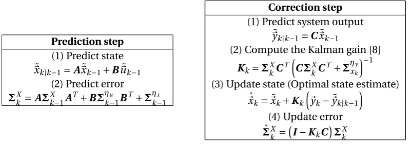
The algorithm used is the Kalman Algorithm uses a prediction and correction or update step.

Prediction phase In the prediction phase the previous state estimate is used to estimate the value of the state at the current timestep. Later in the correction phase measurements from a sensor are used refine the prediction and find a more accurate state estimate.

The prediction step is represented by the following equation:

˜

~xk|k°1=A~x˜k°1+B~~uk

For the predicted state estimate, the uncertainty and thus covariance of the predictionßx_k|k°1

also evolves :

Prediction step

(1) Predict state ˜

~xk|k°1=A~x˜k°1+B~u˜k°1

(2) Predict error

ß_kX=AßX_k°1AT+Bߥ_ku_°1BT+ߥ_kx_°1

Correction step

(1) Predict system output ˜

~yk|k°1=C~x˜k°1

(2) Compute the Kalman gain [8] Kk=ßX_kCT

≥

Cß_kXCT+ߥ_xky¥°1

(3) Update state (Optimal state estimate)

§

~xk=~x˜k+Kk

≥

~yk°~y˜k|k°1

¥

(4) Update error

§

ß_kX =°I°KkC¢ß_kX Table 2.2:Kalman filter overview

Correction As soon as a new measurement comes in from the sensor the measurement resid-uals are calculated using latest prediction and new measurement:

~sk=~yk°C~xk|k°1

ßS_k=CßX_k|k°1CT+ߥ_ky

The optimal kalman gain now calculated by [8]

Kk=ßX_k|k°1C_kT

≥

ßS_k¥°1

The optimal updated state estimate now is calculated using the Kalman gainKkand the

meas-urement residuals~sk.

§

~xk=~x˜k|k°1+Kk~sk

And uncertainty of the optimal state estimate is update accordingly.

§

ßX_{k =}ßX_k|k°1°KkßS_kK_kT

An overview of the Kalman filter is given in figure 2.2.

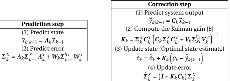
2.6.3 Extended Kalman filter

Because rotations are involved the system cannot be directly written as regular kalman filter because the system behavior is time variant and nonlinear. The different sensors signals are defined in different frames and the there is uncertainty in the relation between these frames. A good solution would be to use an extended kalman filter that linearizes the system every timestep to be able to use the normal equation for a kalman filter.

The state equation is now governed by the non-linear stochastic difference equation:

~xk=f°xk°1,uk°1,¥xk°1

¢

Just as with the regular kalman filter new state can be estimated using the posteriori state es-timate~_kk

°1and the assumption that the mean of the noise is zero.

˜

Prediction step

(1) Predict state ˜

~xk|k°1=Ak~x˜k°1

(2) Predict error

ßX_k =AkßX_k°1A_kT+Wkߥ_kx_°1W_kT

Correction step

(1) Predict system output ˜

~yk|k°1=Ck~x˜k°1

(2) Compute the Kalman gain [8] Kk=ßX_kC_kT

≥

CkßX_kC_kT+VkߥxkyV

T k

¥°1

(3) Update state (Optimal state estimate)

§

~xk=~x˜k+Kk

≥

~yk°~y˜k|k°1

¥

(4) Update error

§

ßX_k =°I°KkCk¢ßX_k Table 2.3:Extended Kalman filter overview

This equation now needs to be linearized

Ak°1=

@f≥~x˜k°1,~uk°1,0

¥

@~x

Wk°1=

@f≥~x˜k°1,~uk°1,0

¥

@~¥xk°1

These same steps can be done for the output equation of the system.

~yk=h°xk°1,uk°1,¥xk°1

¢

˜

~yk=h°xk˜°1,uk°1,0¢

Ck°1=

@h≥~x˜k°1,~uk°1,0

¥

@~x

Vk°1=

@h≥~x˜k°1,~uk°1,0

¥

@~¥xk°1

Combining these equations with the normal deviration of the Kalman filter reasults in the fol-lowing predict and update steps.

It is important to note that a fundamental flaw of the EKF is that the distributions (or densities in the continuous case) of the various random variables are no longer normal after undergoing their respective nonlinear transformations. The EKF is simply an ad hoc state estimator that only approximates the optimality of Bayes rule by linearization [8].

2.6.4 Extended Kalman filter design

For the designed Extended Kalman filter the choice was made not to estimate the rotation in the filter. This was done under the assumption that either the UAV is only making very small rotations which is the case when trying to hoover in place while waiting to be docked.

As first six state variables~xthe position of the drone IMU~pand its velocity ˙~pin the reference frame of the robot base are used. The last three state variables the biases of the accelerometer

~_{ba in its own reference frame are used, which are also estimated by the state estimator. The}

inputs of the system are the body fixed accelerations~ai muand the gravity~g.

~x₌ ~pT~p˙T,~_bT i ,

~

u₌nai mu_{x °}bi mu_x ,ai mu_{y °}bi mu_y ,ai mu_{z °}bi mu_z ,0,0,go

The Kalman matricesAk,Bk,Cmatrices are filled in the following way. TheAkandBkmatrices

are time dependent due to the rotations andIndenotes anRn£nidentity matrix and0na zero

matrix with dimensionsn_£n.

Ak=

2 6 6 4

I3 TI3 03

03 I3 T

h R_igi°1

k 03 03 I3

3 7 7

5 Bk=

2 6 6 4

03 03

ThR_igi

k I3 03 03

3 7 7

5 C=

h

I3 03 03

3 Implementation and Realisation

3.1 Software Implementation : ROS

For implementation of the software the Robotic Operating System framework has been chosen. This is a software framework developed by the Open Source Robotics Foundation [9] and helps developer create complex and robust robotic systems with the help of tools, libraries and an underlying communications framework. The version of the framework used for this Project is the 7th distribution: Hydro Medusa and the operating system that the system is running on is Ubuntu 12.04 LTS.Although the framework runs quite low level the system has no guaran-tees for hard-realtime application because the underlying Linux distribution is not a real-time operating system. The system runs under the highest priority in Linux and can be considered soft-realtime. The system is a Intel I7 2600K with 16 Gb of DDR3 ram.

DUAVRACV brain DUAVRACV

brain KUKA LWR4+

Logitech C920 Xsense MTi OptiTrack AR Parrot drone DUAVRACV Vision Usb_cam (Camera) Xsense (IMU) Ardrone_ Autonomy(imu) DUAVRACV Brain DUAVRACV FRI DUAVRACV Logger Motion capture Node Switch I/O port Computer Vision UAV sensors Robot controller Brain Validation

Figure 3.1:ROS node diagram

The software implementation diagram is shown in figure 3.1. The abbreviation DUAVRACV is used as an affix for the nodes created for this project and stands for “Docking a Unmanned Arial Vehicle using a Robotic Arm and Computer Vision”. The nodes correspond to the subsystem as discussed in the analysis and their relation can be seen in the colored legend. The subsystems for the state estimator and set-point generator are merged into the node called “‘Brain”. The reason for this is that the State Estimator and Set-point generator both needs many signals from the other nodes which would introduce involve a large number of additional topics and extra delays which can be avoided by merging. As can be seen from the diagram there are two possible choices of IMU in the implementation of the system but only one will be used simultaneously. More information about these IMUs and the reasoning behind using a drone substitute is discussed in the hardware realization.

All “DUAVRACV” nodes created for this project will be discussed in their respective paragraphs and the other nodes will be in short explained here.

• USB cam: This node takes camera parameters from a launch file and then starts stream-ing the images to a topic. This is a library from the ROS Wiki and more information can be found athttp://wiki.ros.org/usb_cam

messages on a topic. This is a library from the ROS Wiki and more information can be found athttp://wiki.ros.org/xsens_driver

• Ardone autonomy : This node is used to connect a Parrot AR.Drone over wifi and it posts IMU messages to a topic. The nodes also sends a lot more information and the drone can even be controlled using this node, however these features are not used for this system. This is a library from the ROS Wiki and more information can be found at http://wiki.ros.org/ardrone_autonomy

• Motion capture node : This node is used to connect to the OptiTrack motion capture system that is used for validating the measurements and experiments, it posts pose mes-sages for every “’Trackable’ registered in the OptiTrack system. This is a library from the ROS Wiki and more information can be found athttp://wiki.ros.org/mocap_ optitrack

3.1.1 Brain node

The Brain node is the center of the software system where all the information from the different come together.

The node is build up by a class “Brain” with four member classes that handle different signals. A simplified diagram of the communication in this node is shown in figure 3.2.

Perception StateEstimator

Setpoint Generator

Trajectory Controller Pose

Estimation IMU data

FRI controller

HACK Brain node HACK

Brain State

User Input

Figure 3.2:Brain node diagram

The main brain class connects all the classes together and handles the communication with ROS with the subscriptions and publishers. The arrows in the diagram are pointing the class objects because the messages coming from the other nodes are immediately send to the re-spective class object and not processed in the main class. The user can influence the beha-vior of the controller by means of the “RQT reconfigure GUI” which is a graphical window that allows for parameters of a node to be changed during run time. With this tool the user can (dis)allow behavioral states and change the controller gain or follow distances without restart the node.

Brain State The brain state corresponds to the chosen setpoint generating strategy as dis-cused 2.2.1. Eventhough it is only one variable it is a very important variable in the behavior of the node. To determine the next brain state the brain class takes advise from the other classes which have a better view on current robot pose, distances to the bounds and the and pose es-timation quality. This is done by polling the State Estimator and Setpoint generator every cycle to see what state they would advise for the next iteration cycle. If both advise to go to the next state this is done unless the user input disallows that state from being used.

Perception This object interprets the relative poses messages Hm

c of the pose estimator,

transforms them to the global frameHmg and determines if there are no improbable shifts in

position. The object also keeps track on the success-rate of the last hundred pose estimations which is available for the State Estimator. Because the camera has a delay between the image on the sensor and the time it is processed and in the “Brain” node, not the latest end-effector Hcmpose is used but a older pose that is saved.

Figure 3.3:Dynamic reconfigure GUI

−800

−600

−400

−200

−600

−400

−200

0 ₂₀₀

400 0

100 200 300 400 500 600 700 800 900

Figure 3.4:Reachable subspace approximation

itself, and tranformed into the correct reference frame. The state estimator keeps track of the success-rate of the perception class to determine if the state estimation is still reliable because it is assumed unreliable if there more than 90% estimations where unsuccessful. In this case the pose has been lost for at least 60 frames which corresponds to 3 seconds with a frame rate of 20 hz, the moment that the influence of the acceleration bias becomes significant. When this occurs the state machine is disables and re-initialized when at least 20% of the pose estimates were successful.

Setpoint generator Like described in the analysis the point generator tries generate a set-point according to the know UAV position and behavioral state. The reachable space is defined as a sum of spherical volumes with a center point~piand a radiusri. The process of checking

bounds is done by checking the comparing the distance to all center-points and comparing them to the radii provided. This three dimensional approach does not cover the end-effector orientation but is adequate in preventing the robot to go out of bounds in a dangerous way. In figure 3.4 the subspace is illustrated by the red dots, the green stars are known robot limits.

3.1.2 Robot controller : FRI node

The FRI node controls the robot using the Fast Research Interface (FRI) to communicate with the Kuka Robot Controller (KRC). The FRI node is created around the C++ FRI Library adapted in such a way that it is able to run in the ROS environment and its role is to be a bridge between the KRC and other nodes in the ROS framework. For safety reasons there are rules and proced-ures in the KRC to go through before being allowed to be controlled using FRI and if this is not done correctly the robot is drives are disengaged, stopping the program running on the KRC. The FRI nodes aims be a smooth interface in which the end user only gives the desired (joint) pose, stiffness, etc and the nodes handle the procedure acquiring control over the KRC. The FRI node can handle all three controller strategies provided by KUKA but the report only handles the Cartesian Impedance control mode. The overall FRI connection and setup proced-ures are identical only the contents of the packages is different.

The FRI libraries handles the UDP connection and packages and is used within the FRI node. It should be noted that the FRI library is thread locking and should therefor always run on a separate thread.

FRI Statemachines

The FRI node uses a state-machine in the ROS node and also a state machine running on the KRC to handle the interface connection. The state machine on the KRC always copies the state of the ROS state machine which sends its state as an integer inside the return package to the KRC. The states of the ROS node are: IDLE, INIT, MON, PRECMD, ENDCMN, CMD, KILL. Trans-itions between states are shown in the diagram in figure 3.5.

INIT

IDLE MON

ENDCMD PRECMD

CMD KILL

Figure 3.5:FRI statemachine diagram

The IDLE state is used when no connection is desired.

The INIT initialize the ROS node according to a set of booleans provides which tell it what topics to subscribe and publish to and what commandflags to set in return FRI packages. The node is starts listening to UDP packages coming to the desired ip adress and port. After the connection is established it immidiatly transistions into MON state.

The MON state monitors all the variables coming from the KRC and publishes them on topics. When the different type of control is required the state transitions into INIT mode and when the robot needs to be controlled the state transitions into PRECMD mode.

mode and when this information has reached the ROS statemachine it follows to CMD mode. Monitoring and publishing the KRC variables is done in this mode.

The CMD state controls the robot with the values coming from the topic. Monitoring and pub-lishing the KRC variables is done in this mode. When the different type of control is required the state transitions into ENDCCMD mode.

3.1.3 Data acquisition : DUAVRACV Logger

The logger node is responsible from capturing the desired signals for experiments. It can cap-ture both information from topics or from tranforms that have been broadcasted over the ROS network. The loggers runs at a frequency of 500H zand saves the data to a raw coma sepperated file (.csv). The latest version of the logger logs the following measurements:

• Current pose of the end-effector of the robotic arm.

• The optimal state estimate for the marker pose.

• The pose estimation according to the computer vision.

• The setpoint generated by the setpoint generator (not the intermediate point).

3.2 Hardware realisation

3.2.1 Robotic arm

Figure 3.6:(left) KUKA LWR4+, (right) KRC controller

The robotic arm used for this project is a KUKA LWR4+ robot. This robot is a collaboration between DLR and KUKA to make a lightweight robot that has the capability of reacting compli-antly to outside influences. Merging the best of both DLR and KUKA worlds to obtain the DLR Light Weight Robot (LWR) with the look and feel of an industrial robot.

The novel designs of this robot include the introduction of position sensors on both motor and output side of the joints, torque sensors on the output side of the joints and motor current measurement. Because of this amount of feedback data a compliant controller can be imple-mented which detect external torque which are not coming from the motors or gravity and react to them in a compliant way. The following text is from a KUKA LWR brochure.

“The aluminium housing of the LWR4+ accommodates the motors, gear units, brakes and sensors, as well as the necessary control and power electronics for 7 axes. The result is a powerful, streamlined robot with a payload capacity of 7kg, a compact footprint and minim-ized disruptive contours. Thanks to its integrated sensors, the LWR4+ is extremely sensitive. This makes it ideally suited to handle and assembly tasks. Its low weight of only 16kg makes the robot energy efficient and above all portable. The LWR4+ can thus be easily integrated into ex-sisting systems- either as a fixed installation, or mounted on a moving platform to enable it to perform different tasks at various locations. The LWR4+ is a pilot product for use in reasearch and industrial advance development.”

KRC

The Kuka Robot Controller (KRC) is the system by KUKA to control the LWR4+ robot. It uses a simple programming language to make industrial applications which are mainly fixed pro-grams with occasional input. But the KRC also has a research interface with which the LWR4+ can be directly controlled, this interface is called the “Fast Research Interface” or FRI for short. This FRI interface will be the interface through which all the communication will be done to the robot in this project.

Fast Research Interface

First some terms and variables within the KRC are defined that are required to to understand the workings of the FRI connection.

• FRI Monitor mode: Cyclical communication with transfer of robot data to a remote host, the remote host exchanges data with the KRC but cannot directly the robot.

• FRI Command mode: Cyclical communication with transfer of robot data to a remote host, the remote host can control the robot in this mode.

To control the mode four commands are available to the KRC.

• FRI Open: Opens up the FRI connection by sending out the first UDP package to the remote host.

• FRI Start: Attempt to go into command mode but several checks need to be performed.

• FRI Stop: Stops the command mode and returns to monitor mode

• FRI Close: Closes the FRI connection from monitor mode.

The relation between these command events and the FRI modes can be written into a state chart as can be seen in figure 3.7. The

Figure 3.7:FRI modes transitions chart

The KRC has three different types of strategies to be controlled in while FRI is active.

• Joint position control (code 10): In this mode the joints are controlled in joint space and the robot is acting as stiff as possible.

• Cartesian impedance control (code 20): In this mode the KRC models a six dimensional spring between the setpoint and the end-effector resulting in a force-torque which accel-erates the robot. This is the only cartesian mode because no cartesian position mode is available. With a high stiffness this mode approximates a position control but it has no internal velocity of torque limiting meaning that it will get into torque limit if the desired setpoint is too far away.

• Joint impedance control (code 30): In this mode the joints are controlled by means of a 1 dimensional virtual spring in every joint

unit to the remote host which replies to as fast as possible with UDP message. When the reply is not received before the next package is sent out it is considered lost and the quality of the connection is determined by the succes rate of the UPD package transfer. These packages from the KRC contain a complete set of robot control and status data. A reply message contains input data for the applied controllers.