Application of Model Predictive Control for Improving Stability of Rotor and Controlling Active Rotor Vibration

Application of Model Predictive Control for Improving

Stability of Rotor and Controlling Active Rotor

Vibration

Lipika Sharma

,

Shailja shukla

1

PG Scholar, control system, 2Professors,

Department of Electrical Engineering, Department of Electrical Engineering, Jabalpur Engineering College Jabalpur Engineering College, Jabalpur (M.P) Jabalpur (M.P)

ABSTRACT

The aim of this paper is to study the application of model predictive controller for improving stability of rotor and rotor vibration. Rotor vibrations in electrical machines are dampen out by model predictive control algorithm. The controlled system is the one dimensional Jeffcott-rotor. Model predictive control algorithm was designed, and the simulation results were obtained by Mat lab software tools. Model Predictive Control (MPC) refers to a class of algorithms that compute a sequence of manipulated variable adjustments in order to optimize the future behavior of a plant. In this paper the controlled output of rotor by MPC is further compared with output of same rotor with PID controller.

Keywords

active control of rotor vibration, model predictive control, rotor, PID controller.

1. INTRODUCTION

Rotating machinery is commonly used in many mechanical systems and electrical systems, machine tools, compressors, turbo machinery and aircraft gas turbine engines [1]. Typically these systems are affected by exogenous or endogenous vibrations produced by unbalance, misalignment, resonances, material imperfections, cracks and the electrical point of view vibration produced by system voltage and frequency change. Vibration caused by improving the system losses and minimizes the overall efficiency of the system. This paper introduces the use of Model Predictive Control to dampen rotor vibrations and improving stability of rotor in electrical machines. Model predictive control (MPC) techniques havebeen recognized as efficient approaches to improve operating efficiency and profitability. It has become the accepted standard for complex control problems in the many industries. The controlled object is a rotor supported by journal bearings with a critical frequency of approximately 42 Hz. The dynamics are

characterized by a physical model, and the aim is to control the response of Jeffcott-rotor by constructing a controller that generates control signals that in turn generate the desired output subject to given constraints. Predictive control tries to predict, what would happen to the rotor output for a given control signal. In this way, we know in advance, what effect the control will have, and by this knowledge the best possible control signal is chosen. What is the best possible outcome depends on the given Plant (rotor) and situation, but the general idea is the same

Fig: 1 General View of rotor

2. Mathematical Modeling of Rotor

system

this model at the critical speed the vibration amplitude can reach infinite values. In real machine, very high vibration levels can be reached. Usually largest rotors are operated below the critical speed, but mostly the high-speed rotors are run fast over the critical zone. We can consider the Jeffcott-rotor, this rotor system has only two degrees of freedom (the displacements of the disk in horizontal and vertical directions) or, if we use a rotating co-ordinate system, one: the radial displacement of the disk [3, 4].

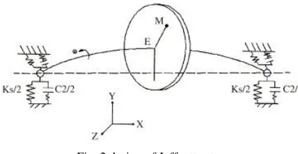
The dynamic characteristics of a rotor dynamic systems system can be studied and analyzed by using simple rotor models. In these models two-degrees-of-freedoms (2-DOF) are considered and assumptions made here are not practical and do not correspond with reality, but they can allow for parametric studies and simplify the solution. These allow us to understand the effects of each parameter on rotor dynamics behaviors. They also provide many valuable physical insights into more complicated systems. Researchers most widely use a single disk centrally mounted on a uniform, flexible shaft, which is supported by two identical bearings, as illustrated in Fig. 2 to study and understand basic rotor-dynamics. If the bearings are infinitely stiff (rigid bearings), this model is normally referred to as the Jeffcott Rotor.

Fig. 2 design of Jeffcott rotor

We can use a complex variable to describe the displacement of the disc centre in the Jeffcott rotor. The displacement in Cartesian coordinate system is

y

= Real(

r

),

y

= Imaginary(

r

),

Where r is the complex radial displacement of the disk in the XY plane. The equation of Motion constant speed of rotation is given by:

+

c

+

kr

=

m

r

ω

e

Where m is the mass of the disk, c is the damping coefficient, k is the spring constant, and are the first and second time derivatives of radial position, m

is equal to unbalancing mass, r is the distance of the unbalance from the geometrical centre of the rotor, ω is the rotational speed, i is the imaginary unit and t is time variable. The undamped critical speed and relative damping can be written as:



(rad/s) ,



=

,



=

In this work the Jeffcott rotor model is used to solve a predictive control problem. The Unbalance response can be formulated as a function of the frequency of rotation.





or in Laplace domain:

G(s) =



Where is the critical angular frequency.

Some numerical simulations were performed using the parameters listed in table 1. [5]

Table 1 Parameters of Jeffcott rotor

Parameter Value

m 0.9 kg

m

k .3 - .05m

C

r

3. Model Predictive Controller

Model Predictive Control (MPC) refers to a class of algorithms that compute a sequence of manipulated variable adjustments in order to optimize the future behavior of a plant. MPC technology can now be found in a wide variety of application areas. The main reasons for such popularity of the predictive control strategies are the intuitiveness and the explicit constraint handling. Several versions of MPC techniques are available. All MPC techniques rely on the idea of generating values for process inputs as solutions of an on-line (real-time) optimization problem. Problem is constructed on the basis of a process model and process measurements. Process measurements provide the feedback element in the MPC structure. In this paper a Model-Based Predictive Control (MCPC) technique is used to control the vibration by designing a controller [3,6].

Figure 3 shows the structure of a typical MPC system. The Model Predictive Control (MPC) is a control algorithm that uses:

• a history of past control moves and

• An optimization cost function J over the prediction horizon, to calculate the optimum control moves.

The algorithm which has to be designed is based on prior knowledge of the model and is independent of it. It is obvious that the benefits obtained will be affected by the differences existing between the real process and the model used [7]. There are various types of techniques are available in MPC. They all are associated with the same idea. The prediction is based on the Model Based Predictive Control (MBPC). The target of the model-based predictive control is to predict the future behavior of the system over a certain horizon using the dynamic model and obtaining the control actions to minimize a certain criterion, generally

Figure3. Model Predictive Control Scheme

J(k, u (k)) = yr ( k + j ))2

+λ 2 (7)

Figure4. Model-Based Predictive Control (MBPC

The Signals y(k + j), yr(k + j), u(k + j) are j-step ahead predictions of the process output, the reference trajectory and the control signal, respectively. The values N1 and N2 are minimal and maximal prediction horizons and Nu is the prediction horizon of control signal. The value of N2 should cover the important part of the step response curve. The use of the control horizon Nu reduces the computational load of the method. The parameter λ represents the weight of the control signal. At each sampling period only the first control signal of the calculated sequence is applied to the controlled process. At the next sampling time the procedure is repeated. This is known as the receding horizon concept. The controller consists of the plant model and the optimization block. Model predictive control is a control strategy that uses a model of the process to predict the response over a future interval, called the prediction horizon [5].MPC uses the receding horizon technique to solve the various problems which is shown in figure 5. In this an internal model is used to predict how the plant will react and start at point k over a prediction horizon.

The l is used to denote the number of steps in the intervals. Each interval has a span of time Ts. so the prediction span

interval is lTs. The prediction depends on the present state

x(k), the disturbance history v and controlled history u. the controlled history which is solved by the MPC is in sum of vector sequences which is represented by m. The interval between two vectors is denoted by Ts. so the control history

span is mTs. During each step the value are held constant

and it is assumed that the values changing simultaneously when new steps changes. When control history ended the controlled value held constant until the predication interval has ended [3, 6].

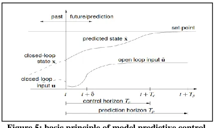
In general, the model predictive control problem is formulated as solving on-line a finite horizon open-loop optimal control problem subject to system dynamics and constraints involving states and controls [8]. Figure 5 shows the basic principle of model predictive control. Based on measurements obtained at time t the controller predicts the future dynamic behavior of the system over a prediction horizon Tp and determines (over a control horizon T) the input such that a predetermined open-loop performance objective functional is optimized. If there were no disturbances and no model-plant mismatch, and if the optimization problem could be solved for infinite horizons, then one could apply the input function found at time t=0 to the system for all times t . However, this is not possible in general. Due todisturbances and model-plant mismatch, the true system behavior is different from the predicted behavior. In order to incorporate some feedback mechanism, the open-loop manipulated input function obtained will be implemented onlyuntil the next measurement becomes available. The time difference between the recalculation/measurements can vary,however often it is assumed to be fixed, i.e the measurement will take place every  sampling time- units. Using thenew measurement at time t+ the whole procedure – prediction and optimization – is repeated to find a new input function with the control and prediction horizons moving forward.

Presenttime Tp

Measurements of process

Current and Future Future process Objective Control action and output Constrains

Disturbance

Now solve the optimization problem

Feasible present and future control

action

Implement the best present control action

Time T= T p+1

Control Algorithm

_Reference

Generator

Optimizer

Model Objective

Function

The input is depicted as arbitrary function of time. For numerical solutions of the open-loop optimal control problem it is often necessary to parameterize the input in an appropriate way. This is normally done by using a finite number of basic functions, e.g. the input could be approximated as piecewise constant over the sampling time .As will be shown, the calculation of the applied input based on the predicted system behavior allows the inclusion of constraints on states and inputs as well as the optimization of a given cost function.

Figure 5: basic principle of model predictive control

4. PID Controller

A proportional-integral-derivative controller (PID controller) is a generic control loop feedback mechanism (controller) widely used in industrial control systems. A PID controller calculates an "error" value as the difference between a measured process and a desired set point. The controller attempts to minimize the error by adjusting the process control inputs. The PID controller calculation (algorithm) involves three separate constant parameters, and is accordingly sometimes called three-term control: the proportional, the integral and derivative values, denoted P, I, and D. These values can be interpreted in terms of time: P depends on the present error, I on the accumulation of past errors, and D is a prediction of future errors, based on current rate of change. The weighted sum of these three actions is used to adjustthe process via a control element such as the position of a control valve, a damper, or the power supplied to a heating element. In the absence of knowledge of the underlying process, a PID controller has historically been considered to be the best controller. By tuning the three parameters in the PID controller algorithm, the controller can provide control action designed for specific process requirements. The PID control scheme is named after its three correcting terms, whose sum constitutes the manipulated variable (MV). The proportional, integral, and derivative terms are summed to calculate the output of the PID controller. Defining u(t) as the controller output, the final form of the PID algorithm is:

U(t)=MV(t)=k

e(t)+k

e(t)

Where

Kp = Proportional gain, a tuning parameter

Ki = Integral gain, a tuning parameter

Kd = Derivative gain, a tuning parameter

e = Error

= SP – PV

t =

T = Variable of integration; takes on values from time 0 to the present .

The proportional term produces an output value that is proportional to the current error value. The proportional response can be adjusted by multiplying the error by a constant kp called the proportional gain constant. The proportional term is given by:

Pout = Kp

A high proportional gain results in a large change in the output for a given change in the error. The contribution from the integral term is proportional to both the magnitude of the error and the duration of the error. The integral in a PID controller is the sum of the instantaneous error over time and gives the accumulated offset that should have been corrected previously. The accumulated error is then multiplied by the integral gain (Ki) and added to the controller output. The integral term is given by:

Iout = Ki

The integral term accelerates the movement of the process towards set point and eliminates the residual steady-state error that occurs with a pure proportional controller. The derivative of the process error is calculated by determining the slope of the error over time and multiplying this rate of change by the derivative gain Kd. The magnitude of the contributionof the derivative term to the overall control action is termed the derivative gain, Kd. The derivative term is given by:

Dout = Kd d/dt e(t)

Derivative action predicts system behavior and thus improves settling time and stability of the system.

5. SIMUTION MODEL AND ANALYSIS

OF RESULT

The transfer function 1-dimensional Jeffcott-rotor which to be controlled in this paper equation 6 is denoted by G(s) [4].

G(s) =



In figure 7 the step response of the rotor model with disturbance is shown. The disturbance is described as a simple sine-wave with same natural frequency as the rotor. The disturbance is defined in such way that a constant value feed to the system causes oscillation to occur between -42Hz and 42Hz. The disturbance for the complete system can be given as one input, one output model [9].

Figure 6: Simulation-step response of rotor model

Figure7: Controlled Output of Rotor with MPC Now the response of 1-dimensional Jeffcott-rotor by using MODEL PREDICTIVE CONTROLLER is shown in figure 7. In figure 6 the step response of rotor with disturbance is showing that the rotor comes in its steady state position after a certain time interval which may be about 500 sec to 600 sec. To overcome with this a model predictive controller is used which reduced the time taken by the rotor i.e it takes only 10 seconds to comes under steady state position which is very small as compare to 500 to 600 seconds which is taken by the rotor without controller.

Figure8: Controlled Output of Rotor with PID Controller

In figure 8, the response of 1-dimensional Jeffcott-rotor by using PID controller is shown in which the controller controls the stability in 50 seconds which is more than MPC.

6. CONCLUSON

7. REFERENCES

[1] SONG Fang-zhen, “Control of Rotor Unbalance Vibration with Magnetic Dynamic Absorber”, IEEE International Conference on Control and Automation Guangzhou, CHINA - May 30 to June 1, 2007, pp no-329-331.

[2] Michael Nikolaou, “Model Predictive Controllers: A Critical Synthesis of Theory and Industrial Needs”, Chemical Engineering Dept, University of Houston, Houston.

[3] Jozef Hrbček, “Active control of rotor vibration by model predictive control” A simulation study, Espoo May 2007, Helsinki University of Technology Control Engineering Laboratory, Report 153.

[4] Kastsuhiko Ogta, “Modern Control Engineering”, 3rd Edition, Published by Prentice Hall.

[5] Dr.Mickael Lallart, “Vibration control”, First Edition published September 2010, Published by Sciyo.

[6] Debadatta Patra “Model predictive control” IIT Rourkela, Bachelor of Technology in Electronics and Instrumentation Engineering, 2007.

[7] A.Vasičkaninova and M. Bakošova, “Neural network predictive control of a chemical reactor”, Proceedings 23rd European Conference on Modelling and Simulation ©ECMS Javier Otamendi, Andrzej Bargiela, José Luis Montes, Luis Miguel Doncel Pedrera (Editors) ISBN: 978-0-9553018-8-9 / ISBN: 978-0-9553018-9-6 (CD)

[8] Abran Alaniz, “Model predictive control with application to real hardware and guided parafoil”, Department of Aeronautics Astronautics , June 2004.

[9] Manfred Morari N. Lawrence Ricker, “Model predictive control tool box”, Version 1, COPYRIGHT 1984 - 1998 by The Math Works, Inc

.