Medical Image Compression Using Wrapping Based Fast Discrete Curvelet Transform and Arithmetic Coding

http://dx.doi.org/10.4236/cs.2016.78179

Medical Image Compression Using Wrapping

Based Fast Discrete Curvelet Transform

and Arithmetic Coding

P. Anandan

, R. S. Sabeenian

1_{Departmentof Electronics and Communication Engineering, R.M.D. Engineering College, Kavaraipettai,}

India

2_{Department of Electronics and Communication Engineering, SONA College of Technology, Salem,}

India

Received 27 March 2016; accepted 20 April 2016; published 30 June 2016

Copyright © 2016 by authors and Scientific Research Publishing Inc.

This work is licensed under the Creative Commons Attribution International License (CC BY).

http://creativecommons.org/licenses/by/4.0/

Abstract

Keywords

Medical Image Compression, Discrete Curvelet Transform, Fast Discrete Curvelet Transform, Arithmetic Coding, Peak Signal to Noise Ratio, Compression Ratio

1. Introduction

The foremost important purpose of image compression is to ease spectral and spatial redundancy to save or to communicate information. Another purpose is to maintain the quality of the image even at lower bit rate to represent an image and to reconstruct it without any degrade in its visual quality. In lossless compression scheme, the reconstructed image will be similar to the original image. In lossy compression scheme, the recon-structed image may not be similar to the original image. But, lossy compression scheme gives higher compres-sion ratio than lossless comprescompres-sion scheme. The proposed scheme is a kind of lossless comprescompres-sion. In the proposed scheme, the coefficients are obtained using second generation of Curvelet Transform. In the quantiza-tion stage, the coefficients carrying least informaquantiza-tion are rounded off. The transform based compression spatial-ly distributes the energy into less number of data samples so that no information is lost. The compressed image is reconstructed into spatial domain by the inverse transformation process [1].

Mohammed Hussien Miry [2] had proposed a novel approach for grayscale image compression using a new hybrid transform, namely Improved Ridgelet Transform. This hybrid transform is based on using Slantlet trans-form instead of wavelet transtrans-form. On different images, compression using Ridgelet transtrans-form was pertrans-formed to obtain comparison results. For natural images, a high quality image compression has been achieved. The im-proved Ridgelet transform is superior and gives faster compression performance when compared to Ridgelet transform approaches. Giridhar Mandyam [3] had proposed a new method for lossless image compression of images using Discrete Cosine Transform. In this method, the high energy coefficients in each block are quan-tized. The number of coefficients used in this method is based on the performance parameters. A. Vasuki [4] had proposed a novel image compression algorithm using the nonlinear Contourlet Transform. Capturing of direc-tional information in images was performed effectively by Contourlets, by using elongated, direcdirec-tional and flexible set of basis functions. Because of the Contourlet transform is redundant, authors have used a contourlet transform based on wavelet on the image. Contourlet transform based on wavelet applies wavelet transform prior to contourlet transform on the sub band of image. It has been shown that the results are superior to ordinary wavelet transform. K. Prasanthi Jasmine has proposed an efficient hybrid combination of wavelet-Ridgelet tech-niques for compression of images. The original image in the RGB color space is converted into grayscale image and to avoid degradation of picture quality due to noise, and denoising of this image is done by Gaussian filter. First DWT (Discrete Wavelet Transform) is applied to the image followed by application of FRT (Finite Ridge-let Transform) to obtain the compressed image. Decompression is done using the inverse FRT and inverse DWT in succession [5]. Veenadevi S. V. has proposed a technique for compressing satellite images using Fractals Transform. In this method, the input image is subdivided into various range and domain blocks. Each range block is matched with domain block. Then affine transformation is applied for each domain block. The im-provement in performance parameters is based on the range block dimensions [6].

Over the past years, several researchers accepted wavelet transform for researches on image compression. Here artifacts are avoided at high compression ratios, but on images with different contents, wavelet decomposi-tion produces poor compression ratio. A new compression technique called CALIC was developed for the pur-pose of context formation, quantization, and modeling. It did not gain popularity because of its poor perfor-mance and complex operation on binary and continuous modes.

The above-mentioned methods are inefficient because they use many number of co-efficient to reconstruct edges along curves and to characterize edge discontinuities along a curve. So in order to overcome these draw-backs a new multi resolution transform called the Curvelet Transform was introduced [7]. This transform is su-perior over wavelet transforms in the cases followed:

In this paper, wrapping based Curvelet Transform is used. The obtained coefficients after transformation are subjected to vector quantization where quantization process happens in a group. Finally, arithmetic encoding is performed to encode stream of characters. The parameters like Compression Ratio and Peak Signal to Noise Ra-tio (PSNR) are measured.

2. Curvelet Transform

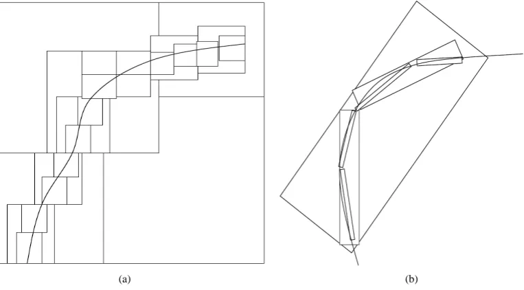
There are several techniques for image compression and observation infers the wavelet may not be the best choice to compress medical image. This is because wavelets have the tendency to ignore edge smoothness. The drawback of wavelet is overcome by the introduction of a technique developed by Candes and Donoho in 1999. This was designed originally to represent edges and curves well than wavelet. The representation of an edge us-ing wavelet is shown in Figure 1(a). Curvelet is an extension of wavelet so there is a relationship between the curvelet and wavelet sub bands [8]. Curvelet Transform elements have location, orientation, and scale, whereas wavelet elements have only location and scale parameters [9][10]. The representation of an edge using curvelet is shown in Figure 1(b). The basic defect of wavelet is the inability to represent the edges and discontinuities along curve and for compression purpose less number of coefficients are involved but for reconstruction process, many in number are needed [11] [12]. This is mainly because to reconstruct the edge discontinuities it needs large number of coefficients.

2.1. Continuous Curvelet Transform

Two generations of Curvelet Transform has been developed. First generations Curvelet Transform (Continuous Curvelet Transform) were obtained from sub band filter theory and Ridgelet theory. The curvelet decomposition takes place in four stages [8]. They are: Sub Band decomposition, Smooth Partitioning, Renormalization and Ridgelet analysis

Ridgelet analysis of radon transform is used in the first generation of Curvelet Transform. Ridgelet transform performance is very slow. Thus, the use of Ridgelet transform was eliminated and a new method to curvelet as tight frame is taken. Using tight frame, an individual curvelet has frequency support in a parabolic wedge area of the frequency domain [13][14].

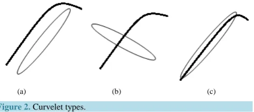
In an experimental argument, all curvelet fall into one of these three categories [8].

1) The magnitude of curvelet coefficient will be zero. Whose discontinuities will not intersect with the length wise support (Figure 2(a)).

2) A curvelet whose discontinuity intersects with length-wise support, but not at its critical angle. At this point magnitude of the curvelet coefficient is approximately equal to zero (Figure 2(b)).

(a) (b)

(a) (b) (c)

Figure 2. Curvelet types.

3) A curvelet whose length-wise support intersects with a discontinuity, at there the curvelet coefficient mag-nitude will be greater than zero. (Figure 2(c))

2.2. Fast Discrete Curvelet Transform

Second generation of Curvelet Transform (Fast Discrete Curvelet Transform) have the advantage of FFT (Fast Fourier transform). Using FFT, the image is represented in Fourier domain [13][15]. In spatial domain, convo-lution of the Curvelet Transform becomes product in their Fourier domain. Curvelet coefficients are obtained by the application of inverse FFT to the spectral product after the end of entire computation process [16].

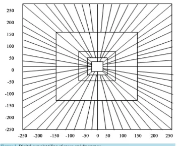
All the coefficients of the orientation and scale are in increasing order. The frequency response of the curvelet is a trapezoidal wedge. The digital curvelet tiling of space and frequency is shown in Figure 3. The wrapping of wedge is obtained using rectangular coefficients, which are collected from surrounding parallelograms. The process of wedge wrapping is called “wrapping based Curvelet Transform”.

2.3. Wrapping Based Fast Discrete Curvelet Transform

In the Curvelet Transform theory, there are two methods to obtain the curvelet coefficients: 1) USFFT (Unequal Space Fast Fourier Transform) method,

2) Wrapping method.

In USFFT method, the coefficients are obtained by irregularly sampling of the Fourier samples of an image. In wrapping method, the coefficients are determined by a sequence of translation and the wrap around technique. Both these methods give same output, but the wrapping based method has better and faster computation time [13]. In this paper, curvelet based on wrapping technique is used.

The oversampled curvelet coefficients is defined by,

(

)

[

]

[

]

1 2

2π ,

1 2 , 1 2 2

, ,

1 _ˆ

, , , , e j j

j

i k n R k n R D O

j n n R

c j k f n n U n n

n + ∈ =

∑

 (1)

where, the superscripts “D” and “O” mention “Digital” and “oversampled”.

Rj,Ɩ is a rectangle of size R1,j × R2,j and containing the parallelogram Pj,Ɩ. If we assume that R1,j and R2,j divide

the image of size n, then the coefficients CD,O(j,Ɩ, k) is obtained by the discrete convolution of a curvelet and the

signal f(t1,t2). Then the coefficients are down sampled regularly in the manner that one selects only one out of

each n/R1,j × n/R2,j pixel. The dimensions R1,j and R2,j of the rectangle are large. In wrapping approach, R1,j and

R2,j are replaced by L1,j and L2,j, the original dimensions of the parallelogram Pj,Ɩ. By copying the data by

wrap-around or periodicity, we can fit Pj,Ɩ into a rectangle with the same dimensions. This is just like relabeling

of the frequency samples of the form,

1 1 1 1,j

n′ = +n m L (2)

2 2 2 2,j

n′ =n +m L (3)

The two dimensional inverse FFT of the wrapped array is of the form,

(

)

(

)

[

]

1 1 1, 2 2 2,

1 2

, ,

2π , 1 2 2

0 0

1 _ˆ

, , , , e j j

L j L j

i k n L k n L D

j

n n

c j k W U f n n

n

− −

+

= =

=

∑ ∑

Figure 3. Digital curvelet tiling of space and frequency.

Note that the relabeling of wrapping does not affect the phase factors. Therefore, we can rewrite the above equation as

(

)

[

] [

]

1 2

2 1 2 1

2π , 1 2 1 2 2 2

ˆ

, , , , e j j

n n

i k n L k n L D

j n n n n

c j k U n n f n n

− − ₊

=− =−

=

∑ ∑

 . (5)

Let consider the mother curvelet at scale “j” and angle “Ɩ” of the form,

( )

( )

( )

,

, 2 ,

1

e d

2π

i x w D

j x Uj

ϕ _ =

_∫

And ϕ#_j, specifies its periodization over the unit square [0, 1]2,

(

)

(

)

1 2

#

, 1, 2 , 1 1, 2 2 D

j j

m Z m Z

x x x m x m

ϕ

ϕ

∈ ∈

=

∑ ∑

  . (7)

The coefficients in the east and west quadrants are given by

(

)

[

]

1 2

1 1

# 1 1 2 2 1 2 ,

2

0 0 1 2

1 , , , , , n n D j t t

t k t k

c j k f t t

n L j n L j

n ϕ − − = =   = + _ − − _  

∑ ∑

 . (8)

This is a discrete circular convolution if and only if L1,j and L2,j both divide n.

Steps for curvelet based on wrapping method

Step 1: Fast Fourier transform (FFT) is applied to input image. Step 2: Curvelet is obtained at given orientation n and scale s. Step 3: Divide the FFT into digitally small sets.

Step 4: Each set is translated to origin for every set. Step 5: Wrap the parallelogram.

Step 6: Apply inverse FFT.

Steps for inverse curvelet based on wrapping method

Step 2: Inverse process is applied to unwrap the rectangular support to the original orientation shape. Step 3: Original position is obtained by translating the shape.

Step 4: The whole curvelet array is stored.

Step 5: All the translated and stored curvelet array are added Step 6: Reconstructed image is obtained by taking Inverse FFT.

3. Algorithmic Approach for Image Compression

Step 1: Image is read from the user.

Step 2: The three level decomposition is used here, discrete curvelet wrapping technique is used to obtain curvelet coefficients.

Step 3: The curvelet coefficient values are quantized so that the approximate values are obtained from this. Step 4: After quantization process, thresholding is applied. The thresholding value is initially set. The coeffi-cient value below the threshold is neglected and above is maintained.

Step 5: Curvelet coefficients above the threshold values are calculated. Step 6: Apply arithmetic encoding technique to encode the coefficients.

Step 7: Inverse Curvelet Transform is achieved by applying Inverse wrapping based algorithm. Step 8: Reconstructed image is obtained from the Inverse Curvelet Transform.

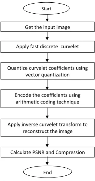
Step 9: Finally, the performance parameters are calculated. Flowchart for the algorithmic approach is shown in Figure 4.

4. Vector Quantization and Arithmetic Coding

Since 1980, Vector Quantization (VQ) is a popular technique. In VQ, inputs are sampled into set of well-defined vectors by the use of some distortion measures. Multimedia images and many other formats of images are used

Figure 4. Algorithmic approach for image

compression.

Start

Get the input image

Apply fast discrete curvelet

Quantize curvelet coefficients using vector quantization

Encode the coefficients using arithmetic coding technique

Apply inverse curvelet transform to reconstruct the image

Calculate PSNR and Compression

in varied applications these days. Storage of multimedia data needs bigger storage. So in order to reduce memo-ry image compression plays a vital role. In quantization large set of inputs are mapped into small set of possible outcomes. Inputs are individual numbers in scalar quantization. Scalar quantization refers to the process of rounding off to the nearest value. The vector input is considered for vector quantization. In VQ, the modeling of probability density functions is done through allocation of prototype vectors. In this method, the large set of vectors is divided into a set which has almost the same number of points [17].

Varieties of techniques are employed for compression having complexities ranging at different degrees. The final step of any compression system is entropy encoding which represents data in a compact manner. This en-coding process may complement the outputs for prior stages. Of all entropy enen-coding techniques, arithmetic coding is the most effective, versatile and an elegant process [18]. The relationship between the actual bits and coded symbols are known in arithmetic coding. Each symbol is assigned to a real-valued number which is coded one at a time [19]. The symbols are then coded in the interval (0,1). Real numbers with fractional digits is the compressed data’s sequence with a code value “v” and equal to the sequence symbols. Codes are formed by padding zeros at the beginning of each coded sequence which interpret the result as a integer value with base-D notation. Here D is coded sequence alphabets number.

5. Performance Parameters

Peak Signal to Noise Ratio is a ratio of the highest signal power and the unwanted noise power. The real image is the signal and the error in re-establishment is the noise. The large Peak Signal to Noise Ratio is used for an enhanced compression. The PSNR is inversely proportional to compression ratio. In order to get actual com-pression, the PSNR and compression ratio should be balanced. The PSNR can be measured using following eq-uation:

( )

(

)

PSNR dB

MSE

×

= . (9)

Mean Square Error is the amount of difference among the real image and the compressed image. MSE is the collective square of difference among the compressed image and the real image. The Mean Square Error should be as low as possible in order to get smaller distortion and large output value. MSE can be measured using fol-lowing equation:

( )

( )

(

)

, ,

MSE

MN

i j f i j −F i j

=

∑ ∑

where,

f(i,j) is the pixel in the input image,

F(i,j) is the pixel in the reconstructed image, M × N is the size of input image.

Compression ratio means the ratio of amount of bits needed to denote the real image to the amount of bits needed to denote the compressed image. If the compression ratio is high then the quality is negotiated. Com-pression methods with no loss of information will have smaller comCom-pression ratio than the lossy comCom-pression methods.

Original Image Size CR

Compressed Image Size

= . (11)

Peak Signal to Noise Ratio and Compression Ratio are the important parameters which are used to determine the quality of any compression algorithm.

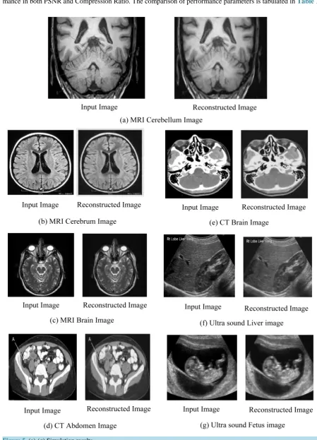
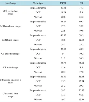
perfor-mance in both PSNR and Compression Ratio. The comparison of perforperfor-mance parameters is tabulated in Table 1.

Figure 6. Comparison of PSNR values in dB.

Figure 7. Comparison of compression ratio values.

6. Conclusion

is our future work.

Table 1. Comparison of performance parameters.

Input Image Technique PSNR CR

MRI cerebellum image

Proposed method 40.32 74.3

DCT 19.28 7.8

Wavelet 20.8 24.2

MRI cerebrum image

Proposed method 35.27 69.3

DCT 17.3 9.12

Wavelet 22.5 19.6

MRI brain image

Proposed method 40.32 74.3

DCT 18.6 12.65

Wavelet 24.7 25.2

CT abdomenimage

Proposed method 37.55 63.3

DCT 14 10.2

Wavelet 21.2 24.5

CT brain image

Proposed method 35.75 55.61

DCT 12.6 8.3

Wavelet 20.3 17.8

Ultrasound image of a fetus

Proposed method 41.80 86.63

DCT 13.5 12.34

Wavelet 25.2 29.3

Ultrasound liver image

Proposed method 39.7 70.32

DCT 14.3 9.36

Wavelet 19.7 12.34

References

[1] Ezhilarasi, P. and Nirmalkumar, P. (2014) A Combined Approach for Lossless Image Compression Technique Using Curvelet Transform. International Journal of Engineering and Technology, 6, 1487-1494.

[2] Miry, M.H. (2008) Image Compression using Improved Ridgelet Transform. Iraqi Journal of Computers, Communica-tions, Control and Systems Engineering, 8, 58-66.

[3] Mandyam, G. and Ahmed, N. (1997) Lossless Image Compression Using the Discrete Cosine Transform. Journal of Visual Communication and Image Representation, 8, 21-26. http://dx.doi.org/10.1006/jvci.1997.0323

[4] Vasuki, A. and Vanathi, P.T. (2009) Progressive Image Compression Using Contourlet Transform. International Journal of Recent Trends in Engineering, 2, No. 5.

[5] Prasanthi Jasmine, K., Rajesh Kumar, P. and Naga Prakash, K. (2012) An Effective Technique to Compress Images through Hybrid Wavelet-Ridgelet Transformation. International Journal of Engineering Research and Applications

(IJERA), 2, 1949-1954.

[6] Veenadevi, S.V. and Ananth, A.G. (2011) Fractal Image Compression of Satellite Imageries. International Journal of Computer Applications, 30, 33-36.

[7] Anandan, P. and Sabeenian, R.S. (2014) Curvelet Based Image Compression Using Support Vector Machine and Core Vector Machine—A Review. International Journal of Advanced Computer Research, 4, 673-679.

[8] Li, Y.C., Yang, Q. and Jiao, R.H. (2010) Image Compression Scheme Based on Curvelet Transform and Support Vec-tor MAchine. Expert Systems with Applications, 4, 3063-3069. http://dx.doi.org/10.1016/j.eswa.2009.09.024

with Edges. Saint-Malo Proceedings,Vanderbilt University Press, Nashville, TN,1-10.

[10] Pandey, K.K. and Suralkar, S.R. (2013) Medical Image Fusion Using Curvelet Transform. International Journal of Electronics and Communication Engineering & Technology, 4, 193-201.

[11] Hamdi, M.A. (2012) A Comparative Study in Wavelets, Curvelets and Contourlets as Denoising Biomedical Images.

International Journal of Image, Graphics and Signal Processing, 1, 44-50. http://dx.doi.org/10.5815/ijigsp.2012.01.06

[12] Elhabiby, M., Elsharkawy, A. and El-Sheimy, N. (2012) Second Generation Curvelet Transforms vs Wavelet Trans-forms and Canny Edge Detector for Edge Detection from WorldView-2 Data. International Journal of Computer Science & Engineering Survey, 3, 1-13.

[13] Candes, E., Demanet, L., Donoho, D. and Ying, L.X. (2005) Fast Discrete Curvelet Transforms. Stanford University.

[14] Gopi, K. and Rama Shri, T. (2013) Medical Image Compression Using Wavelets. IOSR Journal of VLSI and Signal Processing, 4, 01-06. http://dx.doi.org/10.9790/4200-0240106

[15] Donoho, D.L. and Duncan, M.R. (1999) Digital Curvelet Transform: Strategy, Implementation and Experiments. Stanford University.

[16] Saravanan, S, Sujitha Juliet, D. and Shiby Angel, K. (2013) Medical Image Compression Using Modified Curvelet Transform. International Journal of Advanced Research in Computer Science, 4, 70-74.

[17] Rammohan, T, Sankaranarayanan, K. and Rajan, S. (2013) Image Compression Using Fusion Technique and Quantiza-tion. International Journal of Computer Applications, 63, No. 22. http://dx.doi.org/10.5120/10764-5382

[18] Langdon, G.G. (1984) An Introduction to Arithmetic Coding. IBM Journal of Research and Development, 28, 135-149. http://dx.doi.org/10.1147/rd.282.0135

[19] Howard, P.G. and Vitter, J.S. (1991) Practical Implementations of Arithmetic Coding. Proceedings of the International Conference on Advances in Communication and Control, Victoria, British Columbia, Canada, 16-18 October 1991, 1-30.