12
Evaluation of the Performance of Ant Colony
Optimization over Particle Swarm Optimization
S. Padmanabhan
Research Scholar Department of Mechanical and
Production Engineering, Sathyabama University, Chennai,
India
Dr. M. Chandrasekaran
Professor and Director Faculty of Mechanical Engineering
Vels University, Chennai, India
Dr. V. Srinivasa Raman
Professor and Head Department of Mechanical
Engineering
R.V.S. College of Engineering and Technology, Dindigul, India
ABSTRACT
Traditional mathematical algorithms are incapable of solving real time engineering design problems because of its rigid procedure mainly due to discrete or random data and multi-objective functions in a problem. An optimization algorithm is a procedure which is executed iteratively by comparing various solutions till the optimum or a satisfactory solution is found. There are two population based Swarm inspired methods in computational intelligence areas: Ant colony optimization (ACO) and Particle swarm optimization (PSO). This paper made an attempt to evaluate their performance of these two swarm intelligence techniques. A real engineering application of bevel gear design optimization is considered and results are analyzed with respect to the context.
General Terms
Ant Colony Optimization, Gear design, Particle Swarm Optimization.
Keywords
Ant Colony Optimization, Bevel Gear design, Multi Objective Optimization, Particle Swarm Optimization.
1. INTRODUCTION
One of the problems that obstruct the use of engineering optimization in design in the highly specific nature of commonly used numerical algorithms and their inborn limitations. For example, gradient based methods such as Newton Raphson, Bi-section and Secant methods which need differentiable objective function and constraints are the most striking examples of limitations. Also another important limitation is that they can hardly handle discrete variables which are commonly used in mechanical engineering design problems.
Majid Jaberipour and Esmaile Khorram [1] have described about two new harmony search meta-heuristic algorithms for engineering optimization problems with continuous design variables. Lin C et al [2] proposed a new immune algorithm makes use of the PSO advantages to improve the mutation mechanism in the immune algorithm. Wang et al [3] proposed an improved algorithm named bi-directional convergence ant colony optimization (ACO) algorithm based on the graphic definition of the job-shop problem. Davoud Sedighizadeh and Ellips Masehian [4] have surveyed PSO methods and its application. V. Savsani et al [5] have evaluated minimum weight of a spur gear train using particle swarm optimization (PSO) and simulated annealing (SA). Ruifeng Bo et al [6] have analyzed, concept optimization problem based on an Ant Colony System (ACS) and by analyzing the similarity between concept solving and Traveling Salesman Problem.
Zhou et al [7] proposed an ant colony algorithm to solve the prematurity and unsteadiness problem in GA for job shop scheduling with the objective of minimization make span. S. M. Kannan et al [8] have proposed a PSO for minimizing assembly variation in selective assembly problem. Shu-Kai S and Ju-Ming Chang [9] have developed a new proposal of using particle swarm optimization algorithms to solve multi-objective optimization problems was presented. Ju Seok Kang and Yeon-Sun Choi [10] proposed a new method is to optimize the helix angle of a helical gear to minimize the transmission error. Zhang Shaojun et al [11] have describe an optimized model is to formulate the maximization problem on the capacity of V-belt drive. Yin P. Y et al [12] derived a genetic PSO from the original PSO. It was incorporated with the genetic reproduction mechanisms, with crossover and mutation. Rania Hassan et al [13] attempted to examine the claim that PSO has the same effectiveness to finding the true global optimal solution as the GA.
The classical methods are inappropriate when the solution of the problem is computationally intensive. To get Pareto optimal solution for multi objective optimization, these methods have to be employed, many times with different weight or performance vectors [14]. Also these methods can handle either minimization or maximization only. The above difficulties of classical methods can be shorted out by using new Meta heuristics by adopting a Combined Objective Function.
Based on the above observation, this paper has made an attempt to use the potential of Particle swam optimization and Ant colony optimization to solve the bevel gear pair design problem.
2. PARTICLE SWARM OPTIMIZATION
(PSO)
Particle Swarm Optimization (PSO) is a population based stochastic optimization technique developed by Dr. Eberhart and Dr. Kennedy in 1995, inspired by social behavior of bird flocking or fish schooling. It has been applied successfully to wide variety of search and optimization problems. It can be applied to virtually any problem that can be expressed in terms of an objective function.
13
positions in the search space being attracted to both their personal best position as well as the best position found by the swarm so far. The PSO algorithm has shown its robustness and effectiveness in solving function value optimization problems in real engineering design. The attractiveness of the PSO algorithm is due to the features stochastic move, adaptively, and positive feedback.
2.1 Adaptation of PSO
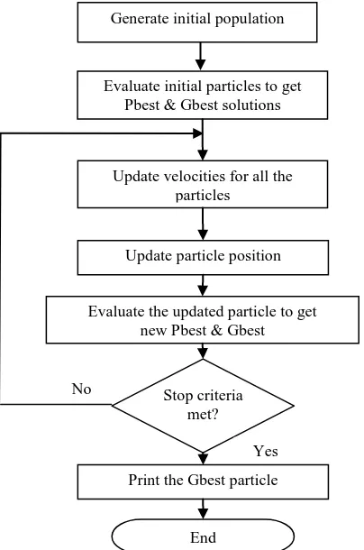
There are two versions for keeping the neighbors best position, namely 1best and gbest. The flow diagram for this algorithm is shown in Fig. 1.[15]
[image:2.595.63.265.350.655.2]In every iteration, each particle is updated by following two “best” values. The first one is best solution it has achieved; its value is called pbest. Another “best” value that is tracked by the particle swarm optimizer is the best value, obtained so far by any particle in the population. This best value is a global best and called gbest. When particle takes part of the population as its neighbors, the best value is the local best and called lbest. In the local population, each particle keeps track of the best position lbest attained by its local neighboring particles. For the global population, the best position gbest is determined by any particles in the entire swarm. Thus the gbest model is a special case of the lbest model. Peng- Yeng Yin [16].
Fig 1: The algorithm for Particle Swarm Optimization
After finding the two best values, the particle updates its velocity and positions with following equation (1) and (2).[17] v[] = ω*v[]+ c l * rand( ) * (pbest []- present[] ) + c2 * rand( )
* (gbest []- present[] ) (1)
present [] = present [] + v[] (2)
Where,
v [] : The velocity for the i th particle , represents the
distance to be traveled by this particle from the current position.
ω inertia weights usually 0.8 to 0.9 .
rand ( ) is a random number between (0,1)
c1, c2 are learning factors .Usually c1 = c2 = 2.
Present []: The location of the ith particle i.e., particle
position.
Pbest []: The best previous position of the ith particle is
recorded and represented as pbest[].
Gbest []: The index of the best particle among all the particles in the population is represented by gbest [].
3. ANT COLONY OPTIMIZATION (ACO)
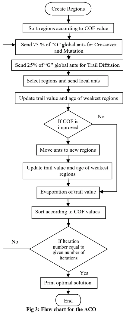
The natural image on which ant algorithms are based is that of ant colony. The cooperative search performance of ants inspires the new algorithm for optimizing engineering design system and is especially suited for solving comprehensive optimization problems Dorigo et al [18]. A bi-level search procedure such as local and global have been introduced and this algorithm is applied for continuous function, it is called as Continuous Ants Colony Algorithm (CACO) Jayaram et al [19]. The distribution of ants is given in Fig. 2 and the flow chart of Ant colony algorithm is shown in Fig. 3. [15]3.1. Global search
The initial solutions or initial regions for ACO are classified into superior and inferior solutions based on their fitness values. Global updates are applied to inferior regions only. The global search for ACO is fairly different from other non-traditional optimization algorithms. The following three steps are to be performed on the randomly generated initial solution. Baskar et al [20].
Random walk (or) Crossover
Mutation
Trail diffusion
3.1.1. Random walk (or) Crossover
[image:2.595.316.537.537.711.2]The crossover and mutation have been carried out in the “G” global ants, where 90% of the solutions are randomly selected in the inferior solutions and are replaced with randomly selected solutions from the superior solutions.
Fig 2: Distribution of Ants for Local and Global search Total no of
Ants 100
No of Global Ants (for inferior
region)
Ratio of Ants 2:3
Ratio of Ants
3.1
No of Local Ants (for superior
region)
No of Ants for Crossover
and Mutation
No of Ants for Trial Diffusion Evaluate initial particles to get
Pbest & Gbest solutions
Update velocities for all the particles
Update particle position
Evaluate the updated particle to get new Pbest & Gbest
Print the Gbest particle Stop criteria
met?
End
Generate initial population
No
14
3.1.2. Mutation
Following to the random walk, at random, add or subtract the value to every variable of the newly created solutions in the inferior region with a probability equal to a properly defined mutation probability. The mutation size is reduced as per the relation
Δ T, R = R (1 − r 1−T b) (3)
Where r is a random number from {0,1}, R is the maximum step size, T is the ratio of the current iteration number to that of the total number of iterations, and b is a positive parameter controlling the degree of non-linearity. The value of b is considered as 10 and determined on a trial basis.
R = Xmax - Xi (4)
Where Xmax is the maximum value in the region
Xi is the current value
3.1.3. Trail Diffusion
In Trail diffusion conducted on 10% of inferior solutions, which were not measured during the random walk and mutation step. Here, two parents are selected at random from the present parent superior solutions.
The variables of the child‟s position vector can have either
the value of the equivalent variable from the first parent;
the equivalent value of the variable of the variable form second parent;
or, a combination arrived from a weighted average of the above
x (child) = (α).xi(parent1) + (1- α).xi(parent2) (5)
Where α is a uniform random number in the range [0,1].
The probability of selecting the third option is set equal to the mutation probability while allotting equal probability of selecting the first two steps. The trail value of the newly created child solutions is assigned a trail value lying between the values of the original parent solutions. The trail values and age of weakest regions are updated [20].
3.2. Local search
The second step in ACO is local search, which is applied as superior solution. The local (artificial) ants select a region i with a probability.
P
it =
τi (t)τt k(t) (6)
Where i is the region index and τi(k) is the pheromone trail on region i at time t.
The best function values are taken from the following steps. After selecting the region, the ant moves through a short distance, the direction of movement is retained if the fitness value progress is observed or else it is reversed. Likewise, the solutions position vector is updated and trail value is enhanced based on the fitness value.
In the ACO algorithm, the pheromone values are decreased after each iteration using the relation,
𝜏𝑖 𝑡 + 1 = 𝜌. 𝜏𝑖 (𝑡) (7)
[image:3.595.325.529.79.599.2]Where ρ is the evaporation rate which is assumed to be 0.2 on a trial basis and 𝜏𝑖 𝑡 is the trail associated with solution at time t. The algorithm executes until the termination criteria is reached and it is the number of iterations by defined the user.
Fig 3: Flow chart for the ACO
4. AN APPLICATION: GEAR DESIGN
The performance of the PSO and ACO are evaluated by taking Bevel gear design as the objective. The gear design problem are taken as, Design a Bevel gear drive to transmit 4kW with the Speed Ratio 4. The input shaft speed is 225 rpm, with non-reversible. This section contains design objectives, objective functions and design constraints are to be discussed.4.1 Design Objectives
The objective functions considered in this application are given below:
Maximization of power delivered by the bevel gear pair (f1)
Jain et al [21].
Send 75 % of “G” global ants for Crossover and Mutation
End Create Regions
Sort regions according to COF value
Send 25% of “G” global ants for Trail Diffusion
Select regions and send local ants
Move ants to new regions
Update trail value and age of weakest regions
Evaporation of trail value
Sort according to COF values
If Iteration number equal to given number of
iterations
No
No If COF is
improved
Update trail value and age of weakest regions
15
Minimization of the overall weight – which is indirectly
related to the volume of the gears (f2) Rao et al [22]. Maximization of the efficiency of the gear pair (f3) [23].
Minimization of the cone distance (f4).Kennady et al [24].
4.1.1 Objective functions
Maximization of power transmitted by bevel gear pair. Eqn. (8) represents this objective function.
f1 = P where , P(L) ≤ P ≤ P(U) (8) Minimization of weight of the bevel gear pair. Eqn. (9)
represents this objective function.
f2 = Weight =
9.24 x 10⁻⁶ 0.2838b3− 1.762m
t Z1 b2+ 3.6369mt2 Z12 b (9)
Maximization of efficiency of gear pair. Eqn. (10) represents this objective function.
f3 = 100 – PL (10)
PL = Power loss and it is expressed by the eqn. (11).
PL= 50 f x coscos Φϴ+cos γ
n x
Hs2+ Ht2
Hs+ Ht
(11) Hs and Ht are calculated by the eqns. (12) and (13) respectively.
HS = i + 1 Ro
R 2
− cos2 Φn − sin Φn (12)
Ht=i+1i ro
r 2
− cos2 Φn − sin Φn (13)
R0=R + one addendum
One addendum for 20o full depth involute system = one average module = mav
Where,
mav = average module of gear and pinion ro = r + mav
Ro = R + mav
𝑟𝑜= 𝑑21+ 𝑚𝑎𝑣
𝑟 = 𝑑1 2
d1= Pitch diameter of the large end of bevel pinion in mm = mt Z1
𝑅𝑜 = 𝑑22+ 𝑚𝑎𝑣
𝑅2= 𝑑2
2
d2= Pitch diameter of the large end of bevel gear in mm = mt Z2 Minimization of cone distance of gear pair. Eqn. (14)
represents this objective function.
𝑓4= 𝑅 = 0.5 mt Z1 i2 + 1 (14)
4.1.2 Design Constraints
The constraints [25] considered in this gear design are given below:
The crushing stress constrain is represented by the expression (15)
Crushing stress : σc< σc (15) The value of induced crushing stress is represented by the equation (16)
σ
c=
R−0.5b0.72i2±1 3 E Mt
ib (16)
The bending stress constrain is represented by the expression (17)
Bending stress: σb< σb (17) The value of induced bending stress is represented by the equation (18)
σ
b=
R i2+1 Mt R−0.5b 2 bmyx
1
cosΦn (18)
Equation (19) represents the gear ratio constraint Gear ratio:
𝑖 = 4 = Z2
Z1 𝑜𝑟
d2
d1 (19)
Equation (20) represents the cone distance constraint
Cone distance : 𝑅 ≥ 𝑅𝑚𝑖𝑛 (20) Where,
Rmin = Minimum cone distance calculated by the formula based on surface Compressive stress.
The minimum cone distance is represented by the eqn. (21).
𝑅𝑚𝑖𝑛 = 𝜓𝑦 i2+ 1 0.72
𝜓𝑦−0.5 σc 2E M
t 𝑖 3
(21)
Ψy = Ratio between the cone distance and face width to calculate the value of „Rmin‟.
The number of teeth constraint is represented by the equation (22)
The number of teeth must be integer:
Zi ε I, for i = 14,15,16,17,18,19,20 (22)
The module constraint is represented by the expression (23) mav ≥ mavmin (23) Where,
mav = average module
mav min = minimum average module calculated by the formula based on bending stress
The minimum average module „mav min‟ is represented by the
eqn. (24).
𝑚𝑎𝑣𝑚𝑖𝑛 = 1.28 𝑦 σ Mt b 𝜓𝑚Z1 3
(24)
16
4.2. Design Objective Function
In this gear pair design problem has four different parameters: maximization of power, minimization of weight of material, maximization of efficiency and minimization of center distance. Since all this parameters are on different scales, in multiple-criterion objective function it is normalized to the same scale [26]. For maximizing criterion value, it is normalized by dividing its value with the normalizing factor, maxi, which is themaximum value of this criterion obtained
from the solutions that have been explored by PSO / ACO so far and for a minimizing criterion value, it is normalized by dividing the normalizing factor, mini, with its value. The
maximum and minimum value of the criterion will be updated whenever the algorithm finds another feasible solution. In addition, to ensure the overall objective value will fall between 0 and 1, the weight of each criterion is also normalized. The normalized objective function can be obtained as follows:
𝐶𝑂𝐹 = 𝑛𝑖=1𝑁𝑊𝑖∗ 𝑁 𝑋𝑖 (25)
Where,
COF Combined objective function Wi prenormalized weight of criterion i.
NWi normalized weight of criterion i.
Where
𝑁𝑊
𝑖=
𝑊𝑖 𝑛𝑖=1𝑊𝑖N(Xi) normalized value of criterion i of solution X.
Where,
𝑁 𝑋𝑖 = 𝑋𝑖
𝑚𝑎𝑥𝑖 for maximizing criterion. (26)
𝑁 𝑋𝑖 = 𝑚𝑖𝑛𝑋 𝑖
𝑖 for minimizing criterion. (27) Xi pre normalizedvalue of criterion X.
maxi best maximum pre normalized value of criterion i of all
solutions so far .
mini best minimum pre normalized value of criterion i of all
solutions so far . N number of criteria.
Hence the COF for bevel gear design is, COF =
power
max. power x NW1 +
min. weight
weight x NW2+ efficiency
max. efficiency x NW3+
min. cent. dist cent. dist x NW4
(28) Where NW1, NW2, NW3 and NW4 = 0.25
5. RESULTS AND DISCUSSION
Mathematical models for the complete problem of bevel gear pair have been formulated in terms of design variables. The optimum values of the objective functions for Power, Weight, Efficiency and Center distance and the design variables (m, b, z and P) influencing the objective functions are obtained with respect to the minimum COF value by implementing the input data provided in Table 1.
Table.1. Data considered in design
Parameter/Constraint Values for bevel gear pair
Material of gear and pinion 40Ni2Cr1Mo 28
Density of the material 8.836×10
6
kg/mm3
Gear ratio 4
Power delivered 4 to 6 kW
Allowable bending stress 400N/mm2
Allowable crushing stress 1100N/mm2
Input speed 225 rpm
Young‟s modulus of the material 2.15x10⁵ N/mm2
Normal pressure Angle 20°
Co-efficient of friction 0.08
Ratio between cone distance and face width to calculate the value of „Rmin‟
(Ψy)
4
Ratio between face width and average module to calculate the value of „mavmin’
(Ψm)
10
[image:5.595.315.538.470.633.2]
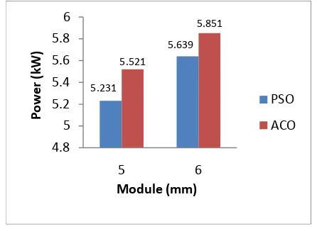
The test bevel gear problem is carried for the module range 4mm to 6mm and the bevel gear design optimization carried by the tools PSO and ACO. The optimized values of required functions are tabulated in the Table 2. From the optimum results, power and weight are compared for ACO and PSO and the chart shown in the figures 4 and 5.
Fig 4: Comparison of Power Transmitted
5.231
5.639 5.521
5.851
4.8 5 5.2 5.4 5.6 5.8 6
5 6
Pow
e
r
(k
W)
Module (mm)
PSO
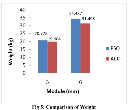
17 Fig 5: Comparison of Weight
It is clearly understood from the figure 4 and 5 that ACO gives the higher Power and lesser Weight while comparing with PSO. The Power gained by 5.5% and 3.5% with respect to 5mm and 6mm modules respectively. Similarly, Weight reduced by 3.9% and 8.7% with respect to 5mm and 6mm modules respectively. Both the tools give the same maximum Efficiency and minimum Cone distance.
6. CONCLUSION
In this paper an attempt has been made to evaluate the performance of Ant Colony Optimization and Particle Swarm Optimization with a real time engineering application. As part of this, bevel gear design is considered and to obtain optimal solution of bevel gear design problem. Within the various design variables available for a gear pair design, the power, weight, efficiency and center distance have been considered as objective functions and bending stress, crushing stress as vital constraints to get an efficient compact and high power transmitting drive. Among the algorithms ACO has produced convincing results for the test problems when compared with the PSO algorithms in the power transmitted and weight reduction of the bevel gear. As a future work, the above tools can be evaluated by optimizing various design application like springs, epicyclic gear train and gear box etc.
7. REFERENCES
[1] Majid Jaberipour , Esmaile Khorram 2010, “Two improved harmony search algorithms for solving engineering optimization problems”, Commun Nonlinear Sci Numer Simulat 15 (2010), pp 3316–3331.
[2] Lin, C., Liu Y., and Lee, C., 2008, “An efficient neural fuzzy network based on immune particle swarm optimization for prediction and control applications”, Journal of Innovative Computing, Information and Control Vol.4, No.7, pp.1711-1722.
[3] Wang C-Q, Cao Y-F, Dai G-Z 2004, “ Bi-directional convergence ACO for job-shop scheduling”, Computer Integrated Manufacturing System Vol.10 (7), pp 820–824.
[4] Davoud Sedighizadeh and Ellips Masehian 2009, “Particle Swarm Optimization Methods, Taxonomy and Applications” International Journal of Computer Theory and Engineering, Vol. 1, No. 5, December 2009.
[5] V. Savsani, R.V. Rao, D.P. Vakharia 2010, “Optimal weight design of a gear train using particle swarm
optimization and simulated annealing algorithms”, Mechanism and Machine Theory , Vol.45, pp 531–541.
[6] Ruifeng Bo, Ruiqin Li and Hongxia Pan 2008, “Concept optimization for mechanical product by using ant colony system”, Journal of Mechanical Science and Technology 22, pp. 628~638.
[7] Zhou P, Li X-P, Zhang H-F 2004 “ An ant colony algorithm for job shop scheduling problem”, Proceedings of the 5th worldcongress on intelligent control and automation, China, 15–19, pp 2899–2903.
[8] S. M. Kannan & R. Sivasubramanian and V. Jayabalan 2009, “Particle swarm optimization for minimizing assembly variation in selective assembly”, Int Jour. Adv Manuf Technology, Vol 42, pp 793–803.
[9] Shu-Kai S. Fan, Ju-Ming Chang 2009, “A parallel particle swarm optimization algorithm for multi-objective optimization problems”, Engineering Optimization, Vol. 41, No. 7, pp 673–697.
[10]Ju Seok Kang and Yeon-Sun Choi 2008, “Optimization of helix angle for helical gear system”, Journal of Mechanical Science and Technology, Vol 22, pp. 2393~2402.
[11]Zhang Shaojun, WAN Zhong and LIU GuangLian 2011, “Global optimization design method for maximizing the capacity of V-belt drive”, Science China Press and Springer-Verlag Berlin Heidelberg, Vol.54 No.1: 140– 147.
[12]Yin, P. Y. 2006, “Genetic particle swarm optimization for polygonal approximation of digital curves” Journal of Pattern Recognition and Image Analysis., Vol. 16, No. 2, pp. 223-233.
[13]Rania Hassan, Babak Cohanim, Olivier de Weck 2004, “A Comparison of Particle Swarm Optimization and the Genetic Algorithm”, American Institute of Aeronautics and Astronautics.
[14]Kalyanmoy Deb and Sachin Jain 2003. “Multi-Speed Gearbox Design Using Multi-Objective Evolutionary Algorithm‟s. Journal of Mechanical design, 125: pp 609-619.
[15]Padmanabhan.S, M.Chandrasekaran and V.Srinivasa Raman 2010, “Optimization of Spur Gear Design Using Metaheuristic Algorithms”, In Proceedings of International Conference on Advances in Industrial Engineering Applications (ICAIEA 2010), Anna University, Chennai.
[16]Peng-Yeng Yin 2006, “Particle Swarm Optimization for point pattern matching”. Journal of Visual Communication and image representation. pp 143- 162.
[17]Kennedy, J. and Eberhart, R. C. 1995, Particle swarm optimization. Proc. IEEE int'l conf. on neural networks Vol. IV, IEEE service centre, Piscataway, NJ. pp. 1942-1948.
[18]Dorigo M, Albert Colorini, 1996, “The ant system: Optimization by a colony of cooperating agents”,IEEE Transaction of Systems, Man and Cybernetics; Part B 26(1), pp1-13.
[19]Jayaram V K, Kulkarni B D, Sachin Karale, Prakash Shelokan, 2000, “Ant Colony Frame Work For Optimal Design And Scheduling Of Batch Plants” , International
20.778
34.487
19.964
31.498
0 5 10 15 20 25 30 35 40
5 6
Wei
gh
t
(k
g)
Module (mm)
PSO
18 Journal of computers and chemical engineering ; vol.24,
pp1901-1912.
[20]Baskar.N, Asokan.P, Saravanan.R and Prabhakaran.G, “Optimization of machining parameters for milling operations using non-conventional methods”, International Journal of Advanced Manufacturing Technology, Vol.25, 2005, pp. 1078-1088.
[21]Jain P, Agogino A M, Theory of design: An optimization perspective. Mech. Mach. Theory 1990; 25 (3), pp.287-303.
[22] Rao S S, Eslampour H R, 1986, “Multi stage multi objective optimization of gear boxes” Journal of mechanisms, Transmissions and Automation in Design, vol.108, pp 461-468.
[23]C. Innocenti, DIEM – University of Bologna, Viale Risorgimento, 2-40136 Bologna, Italy, “A Framework for Efficiency Evaluationn of Multi-Degree-of-Freedom Gear Trains”, Transactions of the ASME, 556 / vol. 118, December 1996.
[24]Deb K, 2005, Optimization for engineering design – algorithms and examples, Eighth Printing, New Delhi, Published by Asoke K. Ghosh, Prentice-Hall of India Private Limited.
[25]Design Data, Faculty of Mechanical Engineering, PSG College of Technology, Coimbatore-641004.
[26]Ying Chin Ho, Colin L. Moodie, 1998, “Machine Layout with a linear Single-RowFlow Path in an Automated Manufacturing System”, Journal of Manufacturing Systems, 17 (1), pp 1 – 22.
Notations
PSO : Particle Swarm Optimization ACO : Ant Colony Optimization
CACO : Continuous Ant Colony Optimization P : Power transmitted in kW
Hs : Specific sliding velocity at start of approach action Ht : Specific sliding velocity at end of recess action. i : Gear (or) transmission ratio
z1, z2 : Number of teeth in pinion, gear d1, d2 : PCD of large end of pinion, gear in mm Ro : Outside radius of large end of bevel gear in mm R2 : Pitch radius of large end of bevel gear in mm
Ro : Outside radius of large end of bevel Pinion in mm r : Pitch radius of large end of bevel Pinion in mm ρ : Density of the material in kg/mm3
E : Young‟s modulus in N/mm2
mt : Transverse Module in mm σc : Induced crushing stress in N/mm2 [σc] : Allowable crushing stress in N/mm2 σb : Induced bending stress in N/mm2
[σb] : Allowable bending stress in N/mm2 b : face with of gear and pinion in mm R : Cone distance in mm.
PL : Percent power loss
[Mt] : Design twisting moment in N mm η : Efficiency, %
y : Form factor