1644
AN EMPIRICAL COMPARISON OF SOME MODIFIED
NEAREST NEIGHBOR RULE FOR CREDIT SCORING
ANALYSIS: CASE STUDY IN INDONESIA
MOCH. ABDUL MUKID, TATIK WIDIHARIH, MUSTAFID
Department of Statistics, Diponegoro University, Semarang, Indonesia [email protected]
ABSTRACT
This paper aims to examine some nonparametric classification methods based on the nearest neighbors rule including k nearest neighbors (KNN), distance weighted k nearest neighbors (DWKNN), local mean k nearest neighbors (LMKNN), and pseudo nearest neighbors (PNN). In order to know the performance of each method, we apply it in case of credit scoring in Indonesia, especially related to a micro credit. For each method studied, we use the same parameter, i.e. the Euclidean distance. After evaluating some odd value k, it is known that each method achieves the optimum classification performance at different k values. KNN achieved the best performance value at k = 11 with total accuracy of 84.91%, while DWKNN achieved best performance at k = 15 which only reached 77.36%. LMKNN works well on k = 9 with an accuracy value of 84.91% and PNN which is a combination between DWKNN and LMKNN only has an accuracy classification of 83.02%. In the case of micro credit in Indonesia with samples from a government bank in Wonogiri district, LMKNN is able to perform better than other methods. With k = 9, the classification performance of LMKNN is the same with the KNN that is obtained at k = 11. Therefore by using LMKNN will reduce the time in determining the label class of a prospective borrower.
Key words: Nonparametric Classification, K Nearest Neighbors, Distance Weighted K Nearest Neighbors, Local Mean K Nearest Neighbors, And Pseudo Nearest Neighbors
1. INTRODUCTION
Micro and small enterprises in Indonesia make an important contributions to economic growth and job creation. In 2017, based on data from Indonesia Central Bureau of Statistics, micro and small enterprises contribute 61.41% of Gross Domestic Product (GDP) and absorb 96.99% of the workforce. However, micro and small enterprises often face obstacles such as lack of information or access to credit or financing, limiting growth and investment opportunities [1]. For empowering Micro Small Medium Enterprises (MSME), job creation and poverty reduction, the Indonesian government issued a micro credit program called Kredit Usaha Rakyat
(KUR). KUR is a credit or working capital financing or investment to individual debtors, business entities and or business groups that are productive and feasible but have not had additional collateral or additional collateral is not enough. MSME that are expected to access KUR are those engaged in productive sectors such as: agriculture, fishery and marine, industry, forestry, and financial services savings and loans. KUR was launched by the the President of the Republic
of Indonesia Susilo Bambang Yudhoyono on November 5th, 2007. In each year, MSME loans have higher growth and generally the growth was higher than total bank credit. The distribution KUR for the year 2016 reached Rp 94.4 trillion, while for the year 2017 reached Rp 96.7 trillion, increasing of 2.4% [2].
The realization of credit usually is done by passing through the process of credit application and credit analysis proposed. Credit expert usually use 5C's analysis i.e. Character, Capacity, Capital, Collateral, Conditional of Economy to assess whether the credit proposed is acceptable or not [3]. With the 5C’s analysis, will be known the ability of borrowers in paying off credit. Unfortunately, this method suffers from high training cost, frequent incorrect decisions, and inconsistent decision made by different expert for the same application [4]. Up to now, statistical models and data mining are two most important methods for credit scoring [5].
There are many data mining algorithms used to credit scoring models, and one of the famous method is k-Nearest Neighbor (KNN).
1645 purposes [6]. In [7], the KNN was claimed to be one of the ten most influential data mining algorithms. The KNN method is a fairly simple method but has a high degree of accuracy. Unfortunately, KNN still has many problems and one of the problems is choosing the right k value.
With majority rule in KNN for choosing large k
values can cause large data distortions because each k-neighbor has the same weight of test data,
while k too small can cause the algorithm to be too sensitive to noise data [8].
The main drawback of the KNN algorithm is that each of k's closest neighbors is equally
important. However, such approach is not always correct, as some farther neighbors may be more important for classification. Distance-Weighted k
-Nearest Neighbor (DWKNN) was developing to overcome the main weakness of the KNN algorithm. The DWKNN method puts the closest neighbor weights greater than the other neighbors that are at a farther distance. Therefore the weight of the function will vary with the distance between the sample and its nearest neighbor, so that when the sample distance with the neighbors increases then the neighbor's weight will decrease [9].
It is also known that nonparametric classifiers suffer from outliers, especially in the situations of small training sample size [10]. That is one reason why the classification performance of KNN rule is heavily influenced by the neighborhood size k [11], [12]. To overcome the
bad effect of outlier, Mitani and Hamamoto developed k nearest neighbor based on local mean. The local mean-based KNN algorithm (LMKNN) is a simple and robust classifier in the small sample size cases. The goal of LMKNN is to reduce the negative effect of the existing outliers in the training set. The reason behind this method is that the local mean vector of k nearest
neighbors in each class is employed to classify the new unlabeled observation in making classification decision [10], [13]. Pseudo Nearest Neighbor (PNN) was created also for both reduce the adverse effect of outliers and decision-making process. This method is a modified KNN and usually used for small data cases [14]. The PNN method basically motivated by distance weighted
k-nearest neighbor rule proposed by Dudani and a
local mean-based nonparametric classifier method proposed by Mitani and Hamamoto [9], [10].
This study compares the performance of several methods based on nearest neighbor rule by using a credit data from a national bank in Indonesia. This paper is organized as follow. In
section 2, we provide the literature review. In section 3, we define data and methodology. In Section 4, we explain our results and discussion. Finally, Section 5 concludes the paper.
2. LITERATURE REVIEW 2.1. Credit Scoring
Credit scoring has been known as a classification method splitting applicants into usually two classes: good credit and bad credit, based on characteristics such as gender, age, education level, occupation, and salary [15]. It consists of the reviewing of the risk related with lending to an organization or an individual [16]. Credit scoring, also known as credit analysis, is carried out by a team or part of the credit organization for the credit application submitted with the aim of assessing the condition of the prospective debtor. This credit analysis is intended so that the credit provision reaches goals that are more directed, yielding, and safe. With the credit analysis, it is expected that the default risk caused by the inability of the debtor to fulfill its obligations as agreed as stated in the credit agreement can be minimized. Inaccurate credit analysis will cause problem loans and will further affect the quality of the bank's loan portfolio. Credit scoring is a set of decision models and basic techniques that help credit lenders in granting credit [17]. Although credit provision has been around for 4000 years, the concept of credit assessment as we know it was developed around 70 years ago. By definition, the purpose of the credit rating model is to identify the profiles of good and bad payers, regardless of the concepts of "good" and "bad".
2.2. K Nearest Neighbor (KNN)
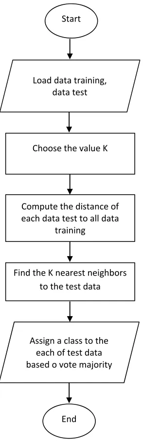
1646 Figure 1 is a fowchart that shows how the KNN algorithm works.
Figure 1 The flowchart of KNN method
To use the k nearest neighbors algorithm, it is necessary to determine the number of k closest neighbors used to classify the new data. The number of k, should be an odd number, for example k = 1, 2, 3, and so on. Determining the value of k is considered based on the amount of data available and the size of the dimensions formed by the data. The more data available, the k number chosen should be lower. However, the larger the dimensions of the data, the k number chosen should be higher.
The classifier assumes the distance of observatios from each other as a criterion for their nearness and selects the most similar observatios. There are numerous methods to compute the distance such as the function of Euclidean distance, Manhattan, etc [20]. The function of Euclidean distance is defined as follows:
D 𝐱𝐢, 𝐱𝐣 x x
, and the function of Manhattan distance is defined as follows:
D 𝐱𝐢, 𝐱𝐣 𝐱𝐢 𝐱𝐣
where 𝐱𝐢 x ,, x , … , x and𝐱𝐣 x ,, x ,
… , x .
2.3. Distance Weighted K Nearest Neighbor (DWKNN)
The main weakness of the KNN algorithm is that each of k's closest neighbors is equally
important. This is unreasonable in some cases because certain neighbors may have more influence than other neighbors. Distance-Weighted k-Nearest Neighbor (DWKNN) was developed to overcome the main drawback of the KNN algorithm. The DWKNN method gives the closest neighbor weights greater than the other neighbors that are at a greater distance than the class unknown. Therefore the weight of the function will vary with the distance between the sample and its nearest neighbor, so that when the sample distance with the neighbors increases then the neighbor's weight will decrease [9].
Suppose given training data 𝑇𝑟
𝐱 , 𝑦 , j =1, 2, …, n with 𝑦 ∈
1,2, … , 𝑐 then di is an Euclidean distance of an object to the nearest neighbor to-j, j=1, …, k
which sorted in increasing order. wi is defined as follows:
𝑤 , 𝑑 𝑑
1, 𝑑 𝑑
which the value of wi varies from maximum 1 for the nearest neighbor to minimum 0 for the farthest neighbor of k. After obtaining the weights of wi, the DWKNN method then gives the class for a new observation, which is the sum of the weights of wi is the largest value. It can be seen from the definition of the weighting function that it is worthy of consideration only for values of k
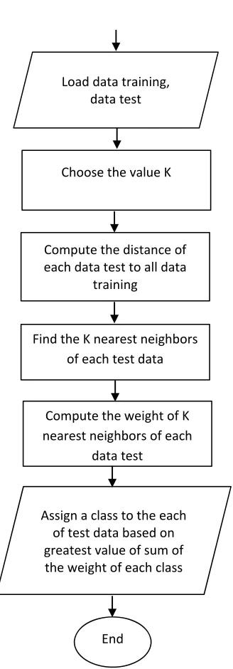
greater than 3. Figure 2 is a flowchart that shows how the DWKNN algorithm works.
Start
Load data training, data test
Find the K nearest neighbors to the test data
Assign a class to the each of test data based o vote majority
End
Compute the distance of each data test to all data
training Choose the value K
1647 Figure 2 The flowchart of DWKNN method
Let wi is the weight of observation to-i, then the sum of the nearest neighbor weights for
wi is defined as follows:
𝑦 ∑ 𝑤 𝐼 𝑦 𝑝 , for p =1, 2, …, c
with 𝐼 𝑦 𝑝 1, 𝑦0, 𝑦 𝑝 𝑝
𝑦 argmax 𝑦 , for p =1, 2, …, c
If the size of the training sample n is very
large compared to the number of nearest neighbors considered, then the results obtained between the two DWKNN and KNN methods will
be comparable to each other. However, the use of the DWKNN method with a small or medium sample of training n will result in a smaller error
probability.
2.4. Local Mean K Nearest Neighbor (LMKNN)
Local mean-based KNN algorithm (LMKNN), is a simple and robust classifier in the small sample size cases. LMKNN was developed to overcome the negative effect of the existing outliers in the training set. The reason behind this method is that the local mean vector of k nearest
neighbors in each class is employed to classify the new observation in making classification decision [10], [13], [21].
Let T 𝐱 ∈ ℝ be a training set of
given m-dimensional feature space, where Nis the
total number of training samples, and y ∈ c , c , … , c denotes the class label for 𝐱 . T
𝐱 ∈ ℝ denotes a subset in Tfrom the class
ci, with the number of the training samples Ni. In the LMKNN rule, the class label of a new observation x is determined by the following steps.
(i) Search the k nearest neighbors from the set T of each class cfor the query pattern x. Let
T 𝐱 𝐱 ∈ ℝ be the set of KNN
for x in the class c using the Euclidean distance metric. Note that the value of k is ≤
Ni.
d 𝐱, 𝐱 𝐱 𝐱 𝐱 𝐱
(ii) Calculate the local mean vector 𝐮 from the class ci, using the set T 𝐱 .
𝐮 1
k 𝐱
(iii) Assign x to the class c if the distance
between the local mean vector for c and the
query pattern in Euclidean space is minimum.
c argmin 𝐱 𝐮 𝐱 𝐮
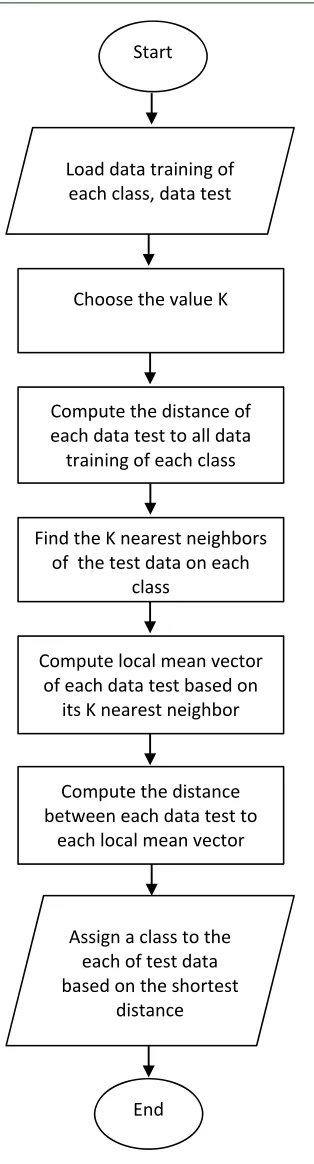
Figure 3 is a flowchart that shows how the LMKNN algorithm works.
Load data training, data test
Find the K nearest neighbors of each test data
Assign a class to the each of test data based on greatest value of sum of the weight of each class Compute the distance of each data test to all data
training Choose the value K
End
Compute the weight of K nearest neighbors of each
1648 Figure 3 The Flowchart Of LMKNN Method
2.5. Pseudo Nearest Neighbor (PNN)
PNN is an improvement of the KNN classification method which is a combination of
local mean-based nonparametric classifier method and distance weighting k-nearest neighbor
[14]. The local mean-based nonparametric learning method proposed by Mitani and Hamamoto aims to overcome the influence of outliers [10]. While the distance weighted k-nearest neighbor is based on the distance where neighbors with the closest distance will have greater weight [9].
In the PNN rule, an unlabeled class of new data x is classified according to the value of the weighted sum of distance of the local k-nearest
neighbor of nearest neighbor selected in each locale or class. Subsequently, the unlabeled data will be classified to local or class whose has minimum value [14]. Suppose that
𝐱 , … , 𝐱 denotes the k-nearest neighbors in
the j-th class data of the unlabeled new data x and j = 1, 2, ... M. While 𝑑 , … , 𝑑 is the corresponding distance arranged in the ascending order by assigning different weights to the closer neighbors having greater weight.
PNN assigns weight to the i-th nearest
neighbor in the j-th class of the unlabeled new
data 𝐱 defined by the weight 𝑤 for 𝑖
1, … , 𝑘. This shown that 𝑤 will decrease with the
increase of value i, the less the value of 𝑤 and 𝑥 which corresponding to that weight has less impact to the classification of unlabeleda new data.
Based on the theory of the local mean learning method of PNN, let 𝑦 be the weighted sum of the distance of k-nearest neighbor of data
x in the j- th class, then 𝑦 is defined as follows:
𝑦 𝑤 . 𝑑 𝑤 . 𝑑 ⋯ 𝑤 .𝑑
where 𝑑 is an Euclidean distance of i-th
nearest neighbor in the j-th class and 𝑤 is the
weight of i-th nearest neighbor. According to [14],
the pseudo nearest neighbor algorithm with the parameter k, as follows :
1. for ( j= 1, 2, .., M )
2. for (i = 1,..., k)
3. calculate the distance between the
k-nearest neighbors of training data in the
j-th class and the test data dj1,...,djk where dji = 𝐱 𝐱
4. end
5. get the arranged distances in increasing order, 𝑑 , … , 𝑑
6. calculate 𝑦 ∑ 𝑤 . 𝑑
7. end
Start
Load data training of each class, data test
Find the K nearest neighbors of the test data on each
class
Assign a class to the each of test data based on the shortest
distance Compute the distance of each data test to all data training of each class
Choose the value K
End
Compute local mean vector of each data test based on
its K nearest neighbor
Compute the distance between each data test to
1649
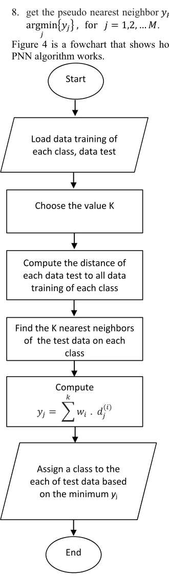
8. get the pseudo nearest neighbor 𝑦
argmin 𝑦 , for 𝑗 1,2, … 𝑀. Figure 4 is a fowchart that shows how the PNN algorithm works.
Figure 4 The Flowchart Of PNN Method
2.6. Evaluation Criteria
The accuracy of a classifier on a given test set is the percentage of test set label that are correctly classified by the classifier. In the pattern recognition literature, this is also referred to as the
overall recognition rate of the classifier, that is, it reflects how well the classifier recognizes the data label of the various classes [22].
The confusion matrix is a useful tool for analyzing how well your classifier can recognize a data of different classes. A confusion matrix for two classes is given m classes, a confusion
matrixis a table of at least size m by m. For a
classifier to have good accuracy, would be represented along the diagonal of the confusion matrixis [23]. From confusion matrix we can measure the accuracy with :
a. Apparent Error Rate
A good classification method will result in a slight misclassification. Apparent Error Rate (APER) is a value used to see the chance of errors in classifying objects. The APER value states the proportion of the misclasification sample is classified. The best method if has the smallest APER value so that the method has the greatest classification accuracy.
APER number of items misclassified
total number of prediction
Accuracy = 1- APER
b. Specificity and Sensitivity
Specificity is a measure of the total number of good borrowers by which a model is classified as a good borrower while sensitivity measures the total bad borrower who is calculated as a bad borrower by the model. Specificity dan sensitivity according to [24] defined as follows:
Specificity % t_pos
pos
Sensitivity % t_neg
neg
t_pos is the number of good borrower which is
classified as good, pos is the number of good
borrower, t_neg is the number of bad borrower
which is classified as bad and neg is the number
of bad borrower
3. DATA AND METHOD
The data used in this paper is a sample of the borrowers of KUR loan in 2016-2017 at a national bank in Wonogiri Regency, Central Java, Indonesia. The size of sample is 265 consist of two classes based on KUR borrower credit status such as good loan (class 1) of 210 data and bad loan (class 2) of 53 data. In this study, the proportion of data is divided into 80% training and 20% testing. This proportion is implemented
Start
Load data training of each class, data test
Find the K nearest neighbors of the test data on each
class Choose the value K
Compute the distance of each data test to all data training of each class
Compute
𝑦 𝑤 . 𝑑
Assign a class to the each of test data based
on the minimum yj
[image:6.612.100.265.88.650.2]1650 in each classes, both in class 1and class 2. Variables used as the basis for the process of credit status classification are age, number of children, long in bussiness, income, loan amount and credit periode.
For some data mining algorithms, differences in the ranges of the data in each variables will lead to a tendency for the variable with greater range will have undue influence on the results. When measuring distance, however certain attributes that have large values, such as income, can overwhelm the influence of other attributes which are measured on a smaller scale, such as number of children. Therefore, to avoid this, the credit analyst should make sure to normalizethe variables values to standardize the scale of effect each variable has on the results. In this study we used the z-score Standardization.
Z-score standardization which is very widespread in the world of statistical analysis, works by taking the difference between the value and the mean value and scaling this difference by the standard deviation of the variable. Let X refer to our original value and Z refer to the normalized value [25].
Z =
One of the most important parameters in the classification method algorithm is k value. In fact, there is no accurate value for k and its proper amount depends on data distribution and space of the problem. For choosing k value can be
determined experimentally, starting with k = 1.
This process can be repeated each time by incrementing k to allow for one more neighbor.
The k value that gives the minimum error rate and
highest accuracy may be selected [26]. We try several k value with odd number to fit the majority
rule based on KNN starting with k=1 untill k=11
depend on amount of datasets.
4. RESULTS AND DISSCUSSION
Applying a credit scoring model is an
attractive activities for both academic researchers
and pratitioners. This study uses data consisting of 265 KUR borrowers with 79.62% of them are good borrower status and the rest are bad borrowers. Descriptive statistics for each variable based on credit status is shown in the Table 1 as follows.
The average age of good borrowers is
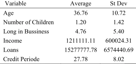
39.94 which tends to be higher than those who are bad borrowers with 36.76 years of age where the standard deviations are 10.93 and 10.72 respectively. This means that there is a possible
relationship between the age of the borrower and the potential of his credit status. If the borrower's age gets bigger then the potential for stuck in lending is getting smaller. The same conditions occur in other variables i.e the long in business, income and loan amount. Meanwhile, the number of children held by both types of credit status is relatively the same with the standard deviation of the good borrower is lower than the bad borrower. Furethemore, the variable credit periode has a situation that is not much different from the number of children in terms of comparison value of borrower characteristics of both credit status good and bad.
Table 1. Description Of Variables For Good Borrower
Variables Average St Dev
Age 39.94 10.93
Number of Children 1.27 0.95
Long in Bussiness 6.44 5.41
Income 1412436.02 896415.84
Loans 18687203.79 7076909.28
[image:7.612.324.542.396.500.2]Credit Periode 27.95 8.17
Table 2. Description Of Variables For Bad Borrower
Variable Average St Dev
Age 36.76 10.72
Number of Children 1.20 1.42
Long in Bussiness 4.76 5.40
Income 1211111.11 600024.31
Loans 15277777.78 6574440.69
Credit Periode 27.78 8.02
In this study, we apply some of modified KNN algorithm as a credit scoring model such as, DWKNN, LMKNN, and PNN methods. The rule of the nearest neighbor specifies the class label of the new observation by a majority vote of the class of its nearest neighbors. Therefore in order to determine the parameters k, we try some odd values. This was done to avoid getting the same number of votes between good class and bad class. After trying with several k value to get the
1651 Table 3. The Accuration Of K-Nearest Neighbor
k Sensitivity Specificity Accuracy
1 0,7381 0,5455 0,6981
3 0,7619 0,5455 0,7170
5 0,7857 0,5455 0,7358
7 0,8333 0,2727 0,7170
9 0,9048 0,1818 0,7547
11 0,9762 0,3636 0,8491
13 0,9524 0,2727 0,8113
15 0,9762 0,2727 0,8302
Table 3 explains the accuracy of KNN method for credit scoring analysis. The sensitivity value of this method tends to fluctuate as the value of k increases but overall in increasing trend. When k = 1 the sensitivity value is 0.7381, whereas for k = 3 its sensitivity value rises to 0.7619. These values will continue to rise up to a value of k = 11 with a sensitivity of 0.9762. However the sensitivity value will decrease for k = 13 and then rise again for k = 15. In contrast, the specificity value of the KNN method tends to fall down although also in fluctuating condition. For k = 1 the specificity value is 0.5455 and this is the greatest specificity value. The lowest specificity value is reached when k = 9 where the value is 0.1818. However, using total accuracy, this method is able to show the best performance at k = 11 with total accuracy reach 0.8491. This means that the KNN method is able to classify properly for both the good borrower and the bad borrower of 84.91%. At k = 11, specificity value equal 0.9762 which it means that the KNN method when applied to micro credit cases in Indonesia shows the number of good borrowers which by the model are classified as good borrowers is 97.62%. In the same value of k, the sensitivity value is 0.3636 which having interpretation that there are 36.36% of bad debtors by the model is classified as bad debtors.
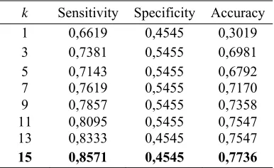
Table 4 shows the values of accuration measures of DWKNN method for credit scoring analysis. In general, the sensitivity value of this method has a positif linear trend as the value of k increases. When k = 1 the sensitivity value is 0.6619, whereas for k = 3 its sensitivity value rises to 0.7381. However at k = 5, the value decrease at level 0.7143 but then the values will continue to rise up to a value of k = 15 with a sensitivity of 0.8571. In contrast, the specificity values of the DWKNN method tend to decrease although also in fluctuating condition. For k = 1 the specificity value is 0.4545 while for k = 3, 5, 7, 9, 11 the value rise up to 0.5455. Unfortunately, at k = 13 and k = 15 have the value lower than 0.5455. In
[image:8.612.324.517.298.416.2]order to determine the parameter k of DWKNN, we use total accuracy as the basis. This method has the best performance at k = 15 with total accuracy reach 0.7736. This means that the KNN method is able to classify properly for both the good borrower and the bad borrower of 77.36%. At k = 15, specificity value equal 0.8571 which it means that the DWKNN method when applied to micro credit cases in Indonesia shows the number of good borrowers which by the model are classified as good borrowers is 85.71%. In the same value of k, the sensitivity value is 0.4545 which having interpretation that there are 45.45% of bad debtors by the model is classified as bad boroower.
Table 4. The Accuration Of Distance Weighted K-Nearest Neighbor
k Sensitivity Specificity Accuracy
1 0,6619 0,4545 0,3019
3 0,7381 0,5455 0,6981
5 0,7143 0,5455 0,6792
7 0,7619 0,5455 0,7170
9 0,7857 0,5455 0,7358
11 0,8095 0,5455 0,7547
13 0,8333 0,4545 0,7547
15 0,8571 0,4545 0,7736
DWKNN was created to improve the decision-making of class labels from new observations of the KNN method by weighting the k of its nearest neighbors. In this way the classification performance is expected to be improved. However, in the case of micro credit in Indonesia, DWKNN did not show better performance than KNN. The best DWKNN performance was achieved when k = 15 while KNN's best performance was achieved when k = 11. Regardless of pamater k, the total value of DWKNN accuracy is only 77.36% lower than KNN's where the accuration is 84.91%. We suspect, maybe this is due to the way of weighting in DWKNN that does not reflect the conditions in this case. The greatest weight may not be on the first nearest neighbor nor the lowest weight not at its last nearest neighbor.
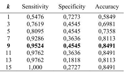
1652 method looks variative. For k = 1 the specificity value is 0.7273 and then the value continues to decrease until 0.3636 that is reached at k = 7. The lowest specificity value is reached when k = 13 where the value is 0.1818. However, using total accuracy, this method is able to show the best performance at k = 9 with total accuracy reach 0.8491. This means that the LMKNN method is able to classify properly for both the good borrower and the bad borrower of 84.91%. At k = 9, specificity value equal 0.9524 which it means that the LMKNN method when applied to micro credit cases in Indonesia shows the number of good borrowers which by the model are classified as good borrowers is 95.24%. In the same value of k, the sensitivity value is 0.4545 which having interpretation that there are 45.45% of bad debtors by the model is classified as bad debtors.
Table 5. The Accuration Of Local Mean Based K-Nearest Neighbor
k Sensitivity Specificity Accuracy
1 0,5476 0,7273 0,5849
3 0,7619 0,4545 0,6981
5 0,8095 0,4545 0,7358
7 0,9286 0,3636 0,8113
9 0,9524 0,4545 0,8491
11 0,9762 0,3636 0,8491
13 0,9762 0,1818 0,8113
15 1,000 0,2727 0,8491
The LMKNN method is built to reduce the adverse effect of the outliers that may affect the classification performance of the KNN method. When new observations are not yet known its class label, the neighbors of the observations are determined in each class of training data, i.e. historical data from a bank that contains both the borrower and the bad borrower. However, in the case of micro credit in Indonesia, LMKNN show a better performance than KNN’s. The best LMKNN performance was achieved when k = 9 while KNN's best performance was achieved when k = 11. Regardless of pamater k, the total value of LMKNN accuracy is the same with KNN's where the accuration is 84.91%. To achieve the best performance, LMKNN requires fewer number of neighbors when compared to the number of neighbors required by KNN. This can speed up the process of computing.
Table 6. The Accuration Of Pseudo Nearest Neighbor
k Sensitivity Specificity Accuracy
1 0,7381 0,5455 0,6981
3 0,7619 0,4545 0,6981
5 0,7619 0,5455 0,7170
7 0,7857 0,5455 0,7358
9 0,8333 0,5455 0,7736
11 0.8810 0,4545 0,7925
13 0,9048 0,3636 0,7925
15 0,9524 0,3636 0,8302
Table 6 talks about the values of accuration measures of PNN method for credit scoring analysis. In general, the sensitivity value of this method has a monotonically increasing as the value of k rising. When k = 1 the sensitivity value is 0.7381, whereas for k = 15 its sensitivity value rises to 0.9524. In contrast, the specificity values of the PNN method tend to decrease although also in fluctuating condition. For k = 1 the specificity value is 0.5455 while for k = 3, 0.4545 and then for k = 5, 7, 9, the value rise up again to 0.5455. Unfortunately, at k = 13 and k = 15, it have only 0.3636. In order to determine the parameter k of PNN, we use total accuracy as the basis. This method has the best performance at k = 15 with total accuracy reach 0.8302. This means that the KNN method is able to classify properly for both the good borrower and the bad borrower of 83.02%. At k = 15, specificity value equal 0.9524 which it means that the PNN method when applied to micro credit cases in Indonesia shows the number of good borrowers which by the model are classified as good borrowers is 95.24%. In the same value of k, the sensitivity value is 0.3636 which having interpretation that there are 36.36% of bad debtors by the model is classified as bad debtore.
[image:9.612.90.289.332.447.2]1653 Fortunately, the total accuration of PNN is greater then DWKNN’s where only 77.36%.
5. CONCLUSSION
Credit scoring analysis needs to be performed by any financial institution in order to reduce the risk of default from the borrower. This analysis is necessary in order to find a borrower with as much potential to smoothly as possible and reduce any decision making errors in determining who is eligible for a loan. Nonparametric classification methods are one of the alternative ways that can be used to assist credit analysts in making decisions regarding proposals from prospective borrowers. The decisions are made on the basis of the borrower's historical data which includes the characteristics of both good and bad borrowers in term of their credit payments. If the characters of the prospective borrower are closer to the credit payment character’s of the good borrower then the prospective borrower's loan proposal is eligible for approval. Conversely, if the prospective borrower has characters that are more similar to a bad borrower then the loan proposal is eligible for rejection.
This study intends to compare several nonparametric classification methods based on the nearest neighboring rules which include KNN, DWKNN, LMKNN, and PNN methods. Parameters that must be specified for the method to work include the distance and size of the neighborhood k. In this study we used Euclidean distance as a measure of the dissimilarity of characteristics among borrowers. The next parameter k is determined by trying some odd values to evaluate its classification abilities in each of the above methods. From this study it is known that the weighting of DWKNN has not been able to improve the classification performance of KNN. In contrast, the average local applied in each class of credit status that becomes the main key in LMKNN method can improve the performance of classification. In the case of this credit assessment in Indonesia, to achieve the same total accuracy, LMKNN requires a total of 9 neighbors when compared to the number of neighbors required in the KNN method. However, the PNN method, which is a combination of weighting in DWKNN and the local average in LMKNN, has not performed better than KNN or LMKNN.
6. ACKNOLEDGMENT
This research was supported by the research and technology and higher education ministry of Indonesia based on contract number 125/SP2H/PTNBH/DRPM/IV/2018.
REFERENCES
[1] BPS, Statistical Yearbook of Indonesia 2018. Jakarta: BPS-Statistics Indonesia,
2018.
[2] K. K. B. P. R. Indonesia, “Kredit Usaha Rakyat,” 2018. [Online]. Available: http://kur.ekon.go.id/gambaran-umum. [Accessed: 20-Aug-2018].
[3] S. E. Kasmir, Dasar-dasar perbankan.
Jakarta: PT Raja Grafindo Persada, 2005. [4] A. I. Marqués, V. García, and J. S. Sánchez,
“Exploring the behaviour of base classifiers in credit scoring ensembles,” Expert Syst. Appl., vol. 39, no. 11, pp. 10244–10250,
2012.
[5] X.-L. Li, “An Overview of Personal Credit Scoring: Techniques and Future Work,” Int. J. Intell. Sci., vol. 02, no. 24, pp. 182–190,
2012.
[6] K. N. Stevens, T. M. Cover, and P. E. Hart,
“Nearest Neighbor Pattern
Classification.pdf,” vol. I, 1967.
[7] X. Wu et al., “Top 10 algorithms in data
mining,” Knowl. Inf. Syst., vol. 14, no. 1, pp.
1–37, Jan. 2008.
[8] D. T. Larose and C. D. Larose, Discovering Knowledge in Data: An Introduction to Data Mining. Wiley, 2014.
[9] S. A. Dudani, “The Distance-Weighted k-Nearest-Neighbor Rule,” IEEE Trans. Syst. Man. Cybern., vol. SMC-6, no. 4, pp. 325–
327, Apr. 1976.
[10] Y. Mitani and Y. Hamamoto, “A local mean-based nonparametric classifier,”
Pattern Recognit. Lett., vol. 27, no. 10, pp.
1151–1159, 2006.
[11] G. Bhattacharya, K. Ghosh, and A. S. Chowdhury, “A probabilistic framework for dynamic k estimation in kNN classifiers with certainty factor,” in 2015 Eighth International Conference on Advances in Pattern Recognition (ICAPR), 2015, pp. 1–
5.
1654 3, pp. 417–423, 2006.
[13] J. Gou, Z. Yi, L. Du, and T. Xiong, “A Local Mean-Based k-Nearest Centroid Neighbor Classifier,” Comput. J., vol. 55, no. 9, pp.
1058–1071, Sep. 2012.
[14] Y. Zeng, Y. Yang, and L. Zhao, “Pseudo nearest neighbor rule for pattern classification,” Expert Syst. Appl., vol. 36,
no. 2, pp. 3587–3595, Mar. 2009.
[15] H. He, W. Zhang, and S. Zhang, “A novel ensemble method for credit scoring: Adaption of different imbalance ratios,”
Expert Syst. Appl., vol. 98, pp. 105–117,
2018.
[16] G. Paleologo, A. Elisseeff, and G. Antonini, “Subagging for credit scoring models,” Eur. J. Oper. Res., vol. 201, no. 2, pp. 490–499,
2010.
[17] L. C. Thomas, D. B. Edelman, and J. N. Crook, Credit Scoring and Its Applications.
Society for Industrial and Applied Mathematics, 2002.
[18] J. Han, J. Pei, and M. Kamber, Data Mining: Concepts and Techniques. Elsevier Science,
2011.
[19] E. Fix and J. L. Hodges, “Discriminatory Analysis. Nonparametric Discrimination: Consistency Properties,” Int. Stat. Rev. / Rev. Int. Stat., vol. 57, no. 3, p. 238, Dec.
1989.
[20] R. A. Johnson and D. W. Wichern, Applied Multivariate Statistical Analysis (Classic Version). Pearson Education Canada, 2018.
[21] J. Gou, H. Ma, W. Ou, S. Zeng, Y. Rao, and H. Yang, “A generalized mean distance-based k-nearest neighbor classifier,” Expert Syst. Appl., vol. 115, pp. 356–372, 2019.
[22] C. R. Rao, Data Mining and Data Visualization. Elsevier Science, 2005.
[23] J. F. Hair, B. J. Babin, R. E. Anderson, and W. C. Black, Multivariate Data Analysis.
Cengage Learning, 2018.
[24] S. Y. Sohn, D. H. Kim, and J. H. Yoon, “Technology credit scoring model with fuzzy logistic regression,” Appl. Soft Comput. J., vol. 43, pp. 150–158, 2016.
[25] H. C. Taneja, Statistical Methods for Engineering and Sciences. I.K. International
Publishing House Pvt. Limited, 2010. [26] D. Mateos-García, J. García-Gutiérrez, and