Explaining Sentiment Classification

Explaining Sentiment Classification

Marvin Rajwadi

, Cornelius Glackin

, Julie Wall

, G´erard Chollet

, Nigel Cannings

1

_{School of Architecture, Computing and Engineering, University of East London, U.K.}

2

_{Intelligent Voice Ltd., London, U.K.}

[email protected], [email protected], [email protected], [email protected], [email protected]

Abstract

This paper presents a novel 1-D sentiment classifier trained on the benchmark IMDB dataset. The classifier is a 1-D convolu-tional neural network with repeated convolution and max pool-ing layers. The main contribution of this work is the demonstra-tion of a deconvoludemonstra-tion technique for 1-D convoludemonstra-tional neural networks that is agnostic to specific architecture types. This deconvolution technique enables text classification to be ex-plained, a feature that is important for NLP-based decision sup-port systems, as well as being an invaluable diagnostic tool.

Index Terms: Explainability, Interpretability, Sentiment

Clas-sification, 1-D Convolutional Neural Networks

1. Introduction

The recent GDPR regulations [1] have important implications for the deployment of real-world customer-facing AI systems. Under these regulations, humans have a right to have decisions explained to them, and this has serious implications for the suit-ability and use of automated AI systems. Coping strategies based on counter-factual explanations [2] have been posited on the one hand, and on the other there is a perception that GDPR is simply incompatible [3] with many of the current practices of deep learning and AI, certainly in their current state. If one considers the rise of end-to-end speech recognition systems as an example, it is commonly understood that such systems have simplified the process of training Automatic Speech Recogni-tion systems. However, if we legally have to explain how such a system arrived at a particular transcription, this would be cur-rently difficult, if not impossible to do, as we would need to un-tangle the decision process from the black-box architecture. As such autonomous deep learning based systems replace humans in the decision making process, it now becomes necessary for AI-based autonomous systems to explain themselves [4].

Arguably by accident, some deep learning architectures have transparency with regard to how they arrive at their clas-sifications, for example the attention mechanism [5] that maps encoder and decoder states provides such insight in neural ma-chine translation. Recent advances with attention have seen a move away from recurrent units entirely for sequence-to-sequence architectures formed entirely of attention mechanisms [6]. The attention mechanism effectively turns the sequence problem into a spatial representation, enabling long-range de-pendencies in sequences to be related more effectively. Simi-larly, activation patterns in convolutional neural network (CNN) architectures can provide insight into CNN classification. Such approaches, termed deconvolution [7], effectively enable the projection of features back to the input space, providing in-sight into what the networksees. For image classification for self-driving cars using CNNs [8] and for hybrid CNN-RNN approaches for image captioning [9], this approach provides

significant diagnostic information. Interestingly, for the image captioning implementation, the explainability is provided by the combined efforts of the attention mechanism and deconvolution functionality.

There are many approaches that try to reverse engineer the inferencing of CNNs, most notable is the recent Grad-CAM im-plementation [10], which is based on guided backpropagation of activation maps. However, most of the activation map-based approaches require intimate knowledge of the particular CNN architecture and the approach needs to be tailored for different architectures.

The method of text deconvolution by occlusion proposed in this paper was inspired by [7], where systematically regions in the input image are occluded by a gray square. That image is inferenced with the trained model, and the shift in classifica-tion accuracy for a particular class is recorded. By overlaying the grid of classification accuracies corresponding to the pixel position of the centre of the occluded squares, one can deter-mine the regions of the input image that contribute the most to the classification of the image as a whole. This approach is computationally demanding in that in order to understand a classification of an image one needs to perform classification of that same input image each with a different occluded region. However, the classification can be run in parallel with multipro-cessing. Similarly, larger strides of the occluded region can be used to limit the computational overhead for 2-D deconvolution by occlusion.

In this paper we will be taking a similar approach to the de-convolution by occlusion approach for 2-D CNNs and applying it to the 1-D text classification problem domain.

2. Sentiment Classification

There is a trade-off between the number of out-of-vocabulary words and vocabulary size that is a significant problem in sequence-to-sequence tasks [11]. In our text classification task, we in part address this problem using word embeddings, and also by capping the number of words in the vocabulary. Whilst for machine translation this limit on vocabulary size might not be suitable, it is less of an issue in this domain as the vocab-ulary size for chat text in the IMDB corpus is significantly smaller than typical written text vocabularies. With this in mind, we choose a word rather than character-based representation as used in [12], and harness the embedding layer to limit this di-mensionality problem. We also avoid the unnecessarily long sequences associated with character-based encoding.

The remainder of this section outlines our approach to sen-timent classification. First we introduce the well-known IMDB dataset, and describe the data preparation performed before pre-senting the 1-D CNN architecture that we will subsequently base our deconvolutional work on.

INTERSPEECH 2019

2.1. IMDB dataset

The IMDB dataset [13] also referred to as the Large Movie Dataset is a binary sentiment analysis dataset consisting of 50,000 highly polar movie reviews, labelled as good or bad re-views. The data was gathered by Stanford researchers and was split evenly between training and testing data with 25,000 ex-amples for each set, and labeled as positive or negative. The dataset contains an even number of positive and negative re-views. A negative review has a score≤4 out of 10, and a posi-tive review has a score≥7 out of 10. No more than 30 reviews are included per movie. Models are typically evaluated based on accuracy, which is sufficient since the data is balanced.

2.2. Data Preparation

Data pre-processing is the most important aspect of training a model, since the quality of the resulting model is directly cor-related with the quality of the data [14]. Raw-text can con-tain significant noise in the form of punctuation and whites-pace. Hence, the first step in pre-processing is cleaning the raw review text, replacing upper-case characters with lower-case, and removing punctuation and whitespace using regular expressions [15]. The second step in pre-processing is to con-vert the clean review text into an input appropriate for our de-fined model, using tokenization. Tokenization is the process of splitting text (strings) into a list of tokens. In this work, we used Tokenizer, which is a tool available in the Natural Language Toolkit (NLTK) [16]. After tokenizing the review text, we use the tokenizer function to create a word index dictionary. The tokenizer function assigns a unique number to the whole vocab-ulary used in the entire dataset in order of the most frequently used words. We have 88,585 unique words used in the IMDB dataset. The review is then converted into a list of correspond-ing word indices and then padded with 0’s to a fixed length for training, as the input must be of similar length. We keep the in-put sequence to a maximum length of 2,000 words and for this particular data-set we use a vocabulary size of 4,000.

2.3. 1-D CNN Architecture

Historically, successively deeper approaches to 2-D CNN ar-chitectures is arguably the main reason for success reported by winners of the ImageNet competition [17]. This pursuit of deeper models has led to a huge surge in applications, and inno-vative approaches to minimizing parameters, improving train-ing efficiency, and has led to better and more robust architec-tures in the image classification [18] domain. The prosperity of deep networks comes from their ability to learn hierarchical feature representations from data which varies in complexity from pixels and lines, all the way to highly complex shapes and objects. However that is not the case when dealing with word representations in the text classification domain. Here deep net-works perform poorly for this particular problem, as the impact of depth in the Natural Language Processing (NLP) domain is still unclear [19].

There has been a lot of debate when it comes to to time se-quence related classifications, what is better a CNN or an RNN? A recent publication in 2017 by Facebook AI demonstrated re-sults using a fully convolutional translation model which out-performs an LSTM based model in performance and reported a speed up of 9x [20]. It is also claimed that due to their hierarchi-cal nature, that CNN architectures learn compositional structure more easily.

In text classification, a previous state-of-the-art approach

embedding_length 128 Embedding

kernal=3, filters =32 pad='same', activation='relu'

Conv1d-1

MaxPooling1D-1 Stride=2

kernal=3, filters =64 pad='same', activation='relu'

Conv1d-2

MaxPooling1D-2 stride=2

kernal=3, filters =32 pad='same', activation='relu'

Conv1d-3

MaxPooling1D-3 stride=2

Fully-Connected-1 output=1024, activation='relu'

Dropout-1 rate=0.5

Fully-Connected-2 output=128, activation='relu'

Dropout-2 rate=0.5

Flatten

Prediction  output=1 activation='sigmoid'

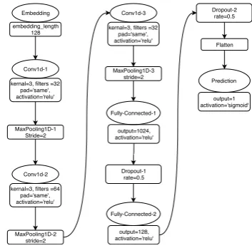
Figure 1:Architecture of the 1-D CNN Sentiment Classifier

used hierarchical attention networks [21] to learn long text se-quences. This approach made use of self-attention, i.e. word-by-word relationships between words in the same sentence, and exploiting that information to capture the internal structure of the sentence. Similarly, hierarchical convolutional attention net-works [22] use self-attention to address the issues with the slid-ing window length of Kim’s CNN architecture [23]. In the orig-inal implementation, Kim uses a sliding window encompassing 4 or 5 words. It is claimed that this means that Kim’s approach is incapable of learning linguistic patterns beyond this 4 or 5 word window size. In this work we do not use a sliding win-dow to maintain a consistent sequence length, neither do we rely on the use of pre-learned embeddings. Instead we employ variable length sequences encoded by an embedding layer that learns embeddings during training, and masks padded elements appropriately from the loss function. We therefore haveno slid-ing window limitation on the length of the sequences that we can learn.

The architecture of the 1-D text classifier in this work is shown in Figure 1. Our architecture validates the conclusion that a relatively shallow CNN with very little hyper-parameter tuning and static vectors can achieve competitive results on sentence-level classification tasks [23]. As can be seen in the figure, our model consists of an embedding layer followed by three Convolutional 1-D layers chained to a ReLU activation layer [24] and MaxPooling 1-D layers. We keep the padding the same throughout all the layers, and we have two fully-connected layers followed by a ReLU activation and a Dropout layer [25] for regularisation, which are attached to the last Maxpooling 1-D layer. The model is compiled using a binary cross-entropy loss function and an RMSprop optimizer with a fixed 1e-3 learn-ing rate and mini batch size of 128. The dense fully connected layers have Sigmoid activation which outputs a number between 0 (negative) to 1 (positive).

be confused with the embeddings that Glove [26] or word2vec [27] learn. These related embeddings are trained to capture se-mantic similarity whilst the Embedding layer in this work out-puts embeddings that are configured purely for classification purposes on the dataset itself [28].

3. Experimentation

First, various pre-processing options that were experimented with are summarised. Following this the training results are benchmarked to other approaches in the literature. The text de-convolution methodology is then presented. Finally, some ex-amples of the capability of the system to explain sentiment clas-sification for various unseen test set examples are presented.

3.1. Pre-processing Text

3.1.1. Stop-words

Removing stop-words is a commonly used method to remove the words that would have little to no impact on the classifica-tion of a sentence. Removing words such as ’I’, ’the’, ’and’, etc., significantly decreases training and inference time. How-ever, this method made no significant difference for this dataset, and for the task of text deconvolution we would require the orig-inal composition of the sentence.

3.1.2. Stemming

This method is used to decrease the vocabulary length of a dataset by mapping similar words such as ’fright’, ’frightened’, ’frightening’ to a same word ’fright’. However adding this mod-ification to our pre-processing step resulted in a decrease in test accuracy. This could be blamed on the nature and perhaps the limited size of the dataset.

3.1.3. Using pre-trained word embeddings

For completeness, we experimented with using pre-trained word embedding weights for the embedding layer. To imple-ment this approach we used ’GloVe’ embeddings [26], which are pre-trained word embeddings computed on the 2014 dump of the English Wikipedia, containing a vocabulary size of 400,000 words.

3.2. Benchmarking

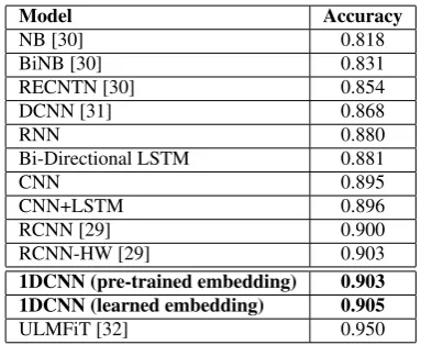
For benchmarking purposes, many model architectures were compared, including recent CNN, RNN and combinations of both (that were implemented by us and found to be consis-tent with results reported in [29]), as well as more traditional Naive Bayes baseline methods reported in [30] and [31]. The same input pipeline and parameters were maintained in an ef-fort to compare like-for-like based on test accuracy. Table 1 summarises the accuracies for this dataset obtained by the dif-ferent models reported in the literature.

The baselines NB and BiNB are Naive Bayes classifiers with, respectively, unigram features and unigram and bigram features. RECNTN [30] is a recursive neural network with a tensor-based feature function, which relies on external struc-tural features given by a parse tree. DCNN [31] is an early con-volutional approach that utilises dynamic k-max pooling where k is determined by the sentence length. As can be seen from Ta-ble 1, the best architecture (our 1DCNN with embedding layer learned from scratch) achieved a 0.905 test accuracy evaluated on 25,000 test reviews. This approach gave slightly better (if

Table 1:Comparison of various architecture approaches

Model Accuracy

NB [30] 0.818

BiNB [30] 0.831

RECNTN [30] 0.854

DCNN [31] 0.868

RNN 0.880

Bi-Directional LSTM 0.881

CNN 0.895

CNN+LSTM 0.896

RCNN [29] 0.900

RCNN-HW [29] 0.903

1DCNN (pre-trained embedding) 0.903

1DCNN (learned embedding) 0.905

ULMFiT [32] 0.950

not statistically significantly better) results than the pre-trained fine-tuned embedding layer. Training was performed using a single NVIDIA GeForce GTX 1080 Ti with 12GB of VRAM. The result shows comparable if slightly less accuracy than the state of the art [32]. However, the main contribution of this pa-per is in the explainability of the inferencing which we will now demonstrate.

3.3. 1-D Deconvolution by Occlusion

Deconvolution by occlusion was originally proposed for image classification problems to identify what part of the input image the network looks at to support the output that it predicts [7]. Using this method, we can tell why the network classifies what it classifies, and if the network has actually trained to identify and distinguish the unique features corresponding to each class. In this paper, we propose the application of the same approach but for the text classification problem. The text deconvolution by occlusion method can be used to visualize the impact of in-dividual words on the final prediction made by the model, see Figure 2 for an example of the output.

What   an   AMAZING!!!   movie,   brilliant   and   outstanding

Occlusion Box

What    an     AMAZING!!!        movie,       brilliant      and     outstanding

Original sentiment : 0.991 Strong Positive

Difference in predicted sentiment after occlusion (delta)

0.991 0.988 0.956 0.982 0.958 0.985 0.968 0.000 0.003

0.04

0.009 0.03

0.006

0.02

(original - delta)

0.05

-0.05

Figure 2:Text Deconvolution with Occlusion

apply this method over the pre-processed text which have had any punctuation or white spaces already filtered out. In this way, this method is agnostic to the architecture of the model itself, since it simply modifies the input data in order to determine the effect of the modification on the output.

An alternative approach to text deconvolution in the liter-ature is termed Text Deconvolution Saliancy (TDS) [33]. This approach is similar to activation map approaches in 2-D CNNs [7] and Layer-wise Relevance Propagation (LRP) [34]. How-ever, like 2-D convolution activation map-based approaches, this approach requires configuration for the particular architec-ture under question.

3.4. Sentiment Inferencing Explained

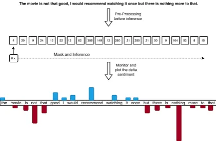
The text deconvolution by occlusion method will now be ex-plained; Figure 3 shows the input pipeline of the inference.

The movie is not that good, I would recommend watching it once but there is nothing more to that.

4 20 9 24 15 52 13 62 386 149 12 280 21 280 21 50 9 164 53 8 15 0 x

the   movie   is   not   that   good   i   would   recommend   watching   it   once   but   there   is   nothing   more   to   that. Pre-Processing

before inference

Mask and Inference

Monitor and plot the delta sentiment

Figure 3:Text Deconvolution Explained

Given an input sentence, we first need to know the senti-ment of the original sentence, then we mask a single number (word) by multiplying it by 0 in the word index sequence gen-erated after the pre-processing stage. By turning an element in the sequence into 0, the network only considers the rest of the words when making the classification. The new masked se-quence is used for inference and we plot the difference between the original sentiment classification and the new occluded sen-timent produced by inferencing each masked word index se-quence. This process is repeated for each and every integer (corresponding to a word) in the sequence, and the plotted out-put gives a visualisation of the impact of each word within the input sentence, and thus contributes towards the explainability of the model’s prediction.

Figure 4 shows the deconvolution at work on a few chosen reviews with their corresponding sentiment, (a) and (b) are sim-ple reviews that contradict each-other with (a) being highly pos-itive and (b) highly negative. These two examples demonstrate the ability of the 1D CNN to learn the context that the words are within, in (a) ’absolutely’ is positive because of its relationship with ’brilliant’, but in (b) ’absolutely’ is negative because of the negative context of the rest of the sentence. (c) shows negation in a sentence, and illustrates that the model is looking at the sentence as a whole and not simply attributing sentiment to in-dividual words. (d) is a positive sentence but with strong nega-tive words like ’hate’ and ’kill’. However, the model overlooks those words and focuses on the over all sentiment of the sen-tence predicting it as positive. This text example is the only one manufactured by the authors as an antogonistic attempt to test the model, all the other reviews are taken from the IMDB test

Marked up Text Sentiment

(a) I like this movie, absolutely brilliant 0.9142 (b) I hate this movie, absolutely trash 0.1397 (c) i wish i could say that the movie was good, but it's terrible 0.3414 (d) As a United fan I hate to say it but Salah is a_{him in my team.} great striker, I would kill to have 0.7792

(e) an incomprehensible script when it shouldn't have been dependent on a rather flaky voice over the animation however show real talent quite visually

impressive 0.6559

(f) this is by far thewooden the dialogues are simply stupid and the story is totally brain-dead its worst non english horror movie I've ever seen the acting is not even scary 2 out of 10 from me 0.0009 (g) I have no way of knowing exactly how much is exaggeration , but I've got a _{creepy feeling that the film is closer to the mark than I want to believe} 0.5538

(h) fun movie great for the kids they found it verypredictable but there are a few surprises great entertaining movie to watch if youre somewhat

looking for something just to entertain dont expect to be seeing a classic 0.9689

(i) the stuff dreams are made of a complete retelling of the play as a dream of vengeance will baffle purists but will delight the open minded a superb effort great cinematography acting and script 11 stars 0.9151

(j)

felix in hollywood is a great film the version i viewed was very well restored which is sometimes a problem with these silent era animated films it has some of hollywoods most famous stars making cameo animated appearances a must for any silent film or animation enthusiast

0.9615

Figure 4:Visualisation of Deconvolution

set. Similar behavior can be observed in (e) where the overall negativity of the sentence is overwhelmed by the positive phrase ’quite visually impressive’. (f) is the most negative out of all re-views, here the model demonstrates its ability to learn from the data. The IMDB dataset includes the rating of the movie: and the user’s review includes ’2 out of 10’, which shares the same negativity as the word ’worst’ within the sentence. Similar to this we have another review (i) which is positive and the model predicts it not just because of the positive words but also be-cause it has learned the significance of the numerical rating ’11 stars’. In (g) it is difficult for a human to determine whether the review is positive or negative and this is reflected rightly in the model’s neutral classification. (h) on the other hand is rightly classified as a highly positive review, despite some un-dermining negative phrases. Similarly, in (j) a positive review is correctly predicted despite some negative words that have been correctly put in the context of the sentence.

These results illustrate how well the trained model gener-alises to unseen data. The diagnostic capability of the approach explains how words from candidate sentences can be taken into context by the resulting sentiment classification.

4. Conclusions

In this paper, we have demonstrated how text deconvolution by occlusion can explain how 1-D CNNs automate classifica-tions, providing an important diagnostic tool for debugging mis-classifications and in turn improving training data and network accuracy. Unlike other approaches to deconvolution, for exam-ple Text Deconvolution Saliency [33], which relies on activation map processing, this method is completely independent of the model’s architecture. For text classification systems applied to autonomous decision making, this approach could be vital for justifying how decisions are made.

5. Acknowledgements

6. References

[1] “Regulation (EU) 2016/679 of the European Parliament and of the Council of 27 April 2016 on the protection of natural persons with regard to the processing of personal data and on the free movement of such data, and repealing Directive 95/46/EC (General Data Protection Regulation),”

Official Journal of the European Union, vol. L119, pp. 1–88, May 2016. [Online]. Available: http://eur-lex.europa.eu/legal-content/EN/TXT/?uri=OJ:L:2016:119:TOC

[2] S. Wachter, B. Mittelstadt, and C. Russell, “Counterfactual expla-nations without opening the black box: automated decisions and the gdpr,”Harvard Journal of Law & Technology, vol. 31, no. 2, p. 2018, 2017.

[3] T. Z. Zarsky, “Incompatible: the gdpr in the age of big data,”Seton Hall L. Rev., vol. 47, p. 995, 2016.

[4] L. H. Gilpin, D. Bau, B. Z. Yuan, A. Bajwa, M. Specter, and L. Kagal, “Explaining Explanations: An Overview of Interpretability of Machine Learning,” arXiv e-prints, p. arXiv:1806.00069, May 2018.

[5] D. Bahdanau, K. Cho, and Y. Bengio, “Neural Machine Transla-tion by Jointly Learning to Align and Translate,”arXiv e-prints, p. arXiv:1409.0473, Sep 2014.

[6] A. Vaswani, N. Shazeer, N. Parmar, J. Uszkoreit, L. Jones, A. N. Gomez, L. Kaiser, and I. Polosukhin, “Attention Is All You Need,”

arXiv e-prints, p. arXiv:1706.03762, Jun 2017.

[7] M. D. Zeiler and R. Fergus, “Visualizing and understanding con-volutional networks,” inEuropean conference on computer vision. Springer, 2014, pp. 818–833.

[8] M. Bojarski, P. Yeres, A. Choromanska, K. Choromanski, B. Firner, L. Jackel, and U. Muller, “Explaining How a Deep Neural Network Trained with End-to-End Learning Steers a Car,”

arXiv e-prints, p. arXiv:1704.07911, Apr 2017.

[9] K. Xu, J. Ba, R. Kiros, K. Cho, A. Courville, R. Salakhutdinov, R. Zemel, and Y. Bengio, “Show, Attend and Tell: Neural Im-age Caption Generation with Visual Attention,”arXiv e-prints, p. arXiv:1502.03044, Feb 2015.

[10] R. R. Selvaraju, A. Das, R. Vedantam, M. Cogswell, D. Parikh, and D. Batra, “Grad-CAM: Why did you say that?” arXiv e-prints, p. arXiv:1611.07450, Nov 2016.

[11] M.-T. Luong, I. Sutskever, Q. V. Le, O. Vinyals, and W. Zaremba, “Addressing the Rare Word Problem in Neural Machine Transla-tion,”arXiv e-prints, p. arXiv:1410.8206, Oct 2014.

[12] Z. Wood-Doughty, N. Andrews, and M. Dredze, “Convolutions are all you need (for classifying character sequences),” in

Proceedings of the 2018 EMNLP Workshop W-NUT: The 4th Workshop on Noisy User-generated Text. Brussels, Belgium: As-sociation for Computational Linguistics, Nov. 2018, pp. 208–213. [Online]. Available: https://www.aclweb.org/anthology/W18-6127

[13] A. L. Maas, R. E. Daly, P. T. Pham, D. Huang, A. Y. Ng, and C. Potts, “Learning word vectors for sentiment analysis,” inProceedings of the 49th Annual Meeting of the Association for Computational Linguistics: Human Language Technolo-gies. Portland, Oregon, USA: Association for Computational Linguistics, June 2011, pp. 142–150. [Online]. Available: http://www.aclweb.org/anthology/P11-1015

[14] F. Malik and F. Malik, “Processing data to improve ma-chine learning models accuracy,” Nov 2018. [Online]. Avail-able: https://medium.com/fintechexplained/processing-data-to-improve-machine-learning-models-accuracy-de17c655dc8e

[15] L. Karttunen, J.-P. Chanod, G. Grefenstette, and A. Schille, “Reg-ular expressions for language engineering,” Natural Language Engineering, vol. 2, no. 4, pp. 305–328, 1996.

[16] S. Bird, E. Klein, and E. Loper, Natural language processing with Python: analyzing text with the natural language toolkit. ” O’Reilly Media, Inc.”, 2009.

[17] J. Deng, W. Dong, R. Socher, L.-J. Li, K. Li, and L. Fei-Fei, “Ima-geNet: A Large-Scale Hierarchical Image Database,” inCVPR09, 2009.

[18] A. Krizhevsky, I. Sutskever, and G. E. Hinton, “Imagenet classi-fication with deep convolutional neural networks,” inAdvances in neural information processing systems, 2012, pp. 1097–1105. [19] H. T. Le, C. Cerisara, and A. Denis, “Do convolutional networks

need to be deep for text classification?” in Workshops at the Thirty-Second AAAI Conference on Artificial Intelligence, 2018.

[20] J. Gehring, M. Auli, D. Grangier, D. Yarats, and Y. N. Dauphin, “Convolutional sequence to sequence learning,” arXiv preprint arXiv:1705.03122, 2017.

[21] Z. Yang, D. Yang, C. Dyer, X. He, A. Smola, and E. Hovy, “Hierarchical attention networks for document classification,” in

Proceedings of the 2016 Conference of the North American Chap-ter of the Association for Computational Linguistics: Human Language Technologies. San Diego, California: Association for Computational Linguistics, Jun. 2016, pp. 1480–1489. [Online]. Available: https://www.aclweb.org/anthology/N16-1174

[22] S. Gao, A. Ramanathan, and G. D. Tourassi, “Hierarchi-cal convolutional attention networks for text classification,” in

Rep4NLP@ACL, 2018.

[23] Y. Kim, “Convolutional neural networks for sentence classifica-tion,”arXiv preprint arXiv:1408.5882, 2014.

[24] V. Nair and G. E. Hinton, “Rectified linear units improve restricted boltzmann machines,” inProceedings of the 27th international conference on machine learning (ICML-10), 2010, pp. 807–814. [25] N. Srivastava, G. Hinton, A. Krizhevsky, I. Sutskever, and

R. Salakhutdinov, “Dropout: a simple way to prevent neural net-works from overfitting,” The Journal of Machine Learning Re-search, vol. 15, no. 1, pp. 1929–1958, 2014.

[26] J. Pennington, R. Socher, and C. Manning, “Glove: Global vectors for word representation,” inProceedings of the 2014 conference on empirical methods in natural language processing (EMNLP), 2014, pp. 1532–1543.

[27] T. Mikolov, I. Sutskever, K. Chen, G. S. Corrado, and J. Dean, “Distributed representations of words and phrases and their com-positionality,” inAdvances in neural information processing sys-tems, 2013, pp. 3111–3119.

[28] D. L´opez-S´anchez, J. R. Herrero, A. G. Arrieta, and J. M. Cor-chado, “Hybridizing metric learning and case-based reasoning for adaptable clickbait detection,”Applied Intelligence, pp. 1–16, 2017.

[29] Y. Wen, W. Zhang, R. Luo, and J. Wang, “Learning text represen-tation using recurrent convolutional neural network with highway layers,”arXiv e-prints, p. arXiv:1606.06905, Jun 2016.

[30] R. Socher, A. Perelygin, J. Wu, J. Chuang, C. D. Manning, A. Ng, and C. Potts, “Recursive deep models for semantic compositionality over a sentiment treebank,” inProceedings of the 2013 Conference on Empirical Methods in Natural Lan-guage Processing. Seattle, Washington, USA: Association for Computational Linguistics, Oct. 2013, pp. 1631–1642. [Online]. Available: https://www.aclweb.org/anthology/D13-1170

[31] N. Kalchbrenner, E. Grefenstette, and P. Blunsom, “A convolu-tional neural network for modelling sentences,” arXiv preprint arXiv:1404.2188, 2014.

[32] J. Howard and S. Ruder, “Universal Language Model Fine-tuning for Text Classification,”arXiv e-prints, p. arXiv:1801.06146, Jan 2018.

[33] L. Vanni, M. Ducoffe, D. Mayaffre, F. Precioso, D. Longr´ee, V. Elango, N. Santos, J. Gonzalez, L. Galdo, and C. Aguilar, “Text deconvolution saliency (tds): a deep tool box for linguistic analy-sis,” in56th Annual Meeting of the Association for Computational Linguistics, 2018.