2017 3rd International Conference on Artificial Intelligence and Industrial Engineering (AIIE 2017) ISBN: 978-1-60595-520-9
Contour Error Control Based on Optimal Discrete Controller
Jun-li GAO, Ya TANG, Hui-hua ZHU and Wei CHEN
School of Automation, Guangdong University of Technology, Guangzhou, 510006, China
Keywords: Contour error, Zero phase error tracking controller, Optimal discrete sampling period.
Abstract. An optimal discrete controller is presented in this paper for contour error control using the standard linear quadratic (LQ) method, upon which the offset loss function and the control loss function were considered to attain a relatively good compromise. The weight coefficient for the control loss and the optimal discrete sampling period are garnered, then a zero phase error tracking controller (ZPETC) is designed with the disturbance observer (DOB) to improve the anti-interference capability and the robustness of the system. The proposed methods are capable of enhancing the stability and rapidity of the discrete controller and reducing the contour error of the system. The results may be valuable for various trajectory tracking control applications.
Introduction
Two approaches have been presented in the literature to reduce the contour error in the precise positioning and trajectory tracking control applications [1]. The first approach is to utilize zero phase error tracking controller (ZPETC) and disturbance observer (DOB)[1-5] to improve the tracking precision of single feed shaft, and thereby directly improve the system contour precision; while the indirect approach is to employ cross-coupled controller (CCC) or proportional-integral-differential (PID) controller [6-10], which could provide decoupling compensation for contour error of each feed shaft according to the current contour locus. The first approach proves to be capable of improving the celerity, sensitivity, and precision of the system with the assistance of ZPETC as the feed-forward controller. Nonetheless, a potential problem with this method is that the discrete time of the feed-forward controller may not be determined theoretically, but rather empirically[3,5,12-14]. There should be supposed to be an optimal sampling period in theory for the discrete control, based on which a well discrete controller with the optimal trajectory tracking capacity can be designed.
In this project, an optimal discrete controller was proposed to utilize the standard LQ method, which could reach a good compromise between the offset and the control loss. A weight coefficient for the control loss was garnered, and then the optimal discrete sampling period was determined via carefully balancing the offset and the control loss [15], based on which the control function was discretized, and finally ZPETC was designed and DOB was added to strengthen the anti-interference ability and robustness of the system. The design process was described in this study, and a simulation was performed to verify the applicability and efficacy of the discrete sampling period for the trajectory tracking control.
System Scheme
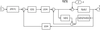
the controller for the closed-loop feedback system, and G(s) represents the corresponding closed-loop transfer function and DOB, respectively.
Figure 1. System control block.
The major processes are as follows: First, the sampling period for the optimal discrete controller is determined based on the trade-off among the control loss function and the offset loss function and the weight coefficient. Second, the control function is discretized based on the calculated optimal discrete sampling period, and then a ZPETC feed-forward controller is designed according to the discretized transfer function. Third, the purpose of adding DOB is to enhance the anti-interference ability and robustness of the system. Fourth, Simulation is performed via Matlab/Simulink.
Optimal Discrete Sampling Period
In a computer control system, all the information needs to be converted into digital signals by the computer. Given that the real control system is a continuous-time system, an approximate continuous-time controller is designed using the shortest possible sampling period. Normally, in most applications, the sampling period should be as short as possible for realizing a better control Nonetheless, in some particular applications, the determination of discrete sampling period needs to consider the trade-off between the control loss function and the offset loss function in the real system. The determination of the optimal discrete sampling period for the contour error control of single shaft is discussed in this section. The motion control of a single shaft Eq. 1. can be described by a single-input/single-output controllable canonical form of transfer function Eq. 2:
1
1 1
1
1 1
( ) ( )
( )
n
n n
n n
n n
b s b s b Y s
G s
U s s a s a s a
(1)
( ) ( ) ( ) ( ) ( )
x t A x t B u t y t C x t
(2) A linear discrete-time controller needs to be designed:
0 ( ) ( ) ( )
u k L T x k (3)
0 0
0 1 0 2 0 0
( ) ( ) ( 1)
( ) ( ( ) ( ) n( ))
u t u k kT t k T L T L T L T L T
(4) T0 is the sampling period and L is the optimal controller that they could minimize the following quadratic continuous loss function:
2 2
0
0 ( ( ) )
J
y p T u d t(5) Eq. 5 can be divided into the offset loss Jy and the control loss Ju:
0 ( ) ( ) ( )
u k L T x k (6)
a given x(0), both Jy and Ju are dependent on T0. Accordingly, the continuous loss functions Eq. 5 and Eq. 6 can be expressed as:
0
0 0
0 0
min ( )
or min( ( ) ( )) ( ) y T y u T u uo J T
J T qJ T J T J
(7)
Ju0 is the extreme of a given control loss, and q is the coefficient obtained eclectically by balancing Jy and Ju.
Selection of Weight Coefficient
In order to minimize Eq.5 at T0, the u(0) needs to satisfy the following condition at t=0:
2 ( 0 ) 2 ( 0 ) 1
2( 0 ) ( 0 )
u u p K y y (8) If the integral loop is not included in the transfer function:
0 2 2 1 2 0 0
( 0 )
( ( 0 ) n) n( 0 )
n T
p p
L a L
T b
(9) If the integral loop is included in the transfer function:
0
2 2 0 0
( 0 ) ( 0 ) ( 0 ) ( 0 )
( 0 )
m T
p u
p L p
T y
(10)
Where
2 (0)
(0) (0)
( 2) (0)
n
n
b K Ku
K G p m
a m m y
(11) When T0≠0, an approximate expression that satisfies the limiting condition described above can be calculated theoretically:
0 0
0 0
( ) (0)(1 )(1 0.3 sin ) 0
2 m
m m
T T
p T p T T
T T
(12) The reference sampling period Tm can be easily approximated. Since p(T0) is not a straight line, Tm can be calculated. If the integral loop is not included in the transfer function:
0
1 0 0 (1 .1 1 .5 ) ( 0 )( )
m T p T p T
(13)
It follows from Eq.9 and Eq.13 that:
2 2 1
(1 .1 1 .5)
(0 )( (0 ) ) (0 )
n m
n n
b T
p L a L
(14) If the integral loop is included in the transfer function:
0 1
0 0
(1 .3 1 .7 ) ( 0 )( ) m T p T p T (15) It follows from Eq.10 that:
1 (1 .3 1 .7 )
( 0 )
m n T L (16)
Selection of Sampling Period
can be determined quantitatively. Admittedly, a potentially troublesome problem is that the calculation is quite complex, and Ju0 or q is tough to be determined in advance. Nevertheless, it is noted that when T0 exceeds a critical value, Jy(T0) will decrease slowly or ever increase instead; besides, when T0 exceeds another critical value, Ju(T0) will increase very rapidly. Thereby T0 can be estimated as:
0 (0.4 0.6) m
T T (17)
The optimal sampling period and weight coefficient that take into account both Jy(T0) and Ju(T0) are determined as:
0 0.5
0.4 (0) m
T T
p p
(18)
The Control Algorithm of ZPETC and DOB The Design of Feed-Forward Controller
ZPETC is proposed based on the idea of pole/zero offset each other by Tomizuka[12], the purpose of which is to improve the tracking precision in the motion control applications. In the tracking control, the real system may not consider the influence of some electromagnetical and mechanical properties, and thus may not respond to the input signals in real time in the simulation or real applications, resulting in the time delay and phase difference of the output. A particular advantage of ZPETC is that the input trajectory signals in the contour tracking control are known in advance, and thereby a feed-forward compensator can be designed, which makes it possible for the output signals to track the input signals in real time, and there is no phase difference in the whole frequency range.
1
1 2
( ) ( ) ( )[ (1)]
d u
a u
z A z B z
B z B
1 1 1 ( ) ( )
( )
d a u
z B z B z A z
*( )
y k u k( ) y k( )
1 ( )
[image:4.612.209.405.406.451.2]C Z T Z( 1)
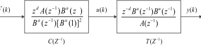
Figure 2. Discrete control block diagram.
The block diagram of the feed-forward controller is shown in Figure 2, where T(z-1) is the discrete transfer function obtained by discretizing the mathematical model of motor using the optimal discrete sampling period, and C(z-1) is the feed-forward controller designed due to the value of T(z-1).
1 1
1
1
( ) ( ) ( )
( )
( ) ( )
d a u
y k z B z B z T z
u k A z
(19) Where y(k) and u(k) are the input and the output of the controlled system, d is the time delay, and respectively, Bu(z-1), Ba(z-1) and A(z-1) are the polynomials of the unstable zeroes, stable zeroes and poles of the discrete transfer function, respectively. Obtained via the discrete transfer function, the zeros and poles of the system, and the input for the contour trajectory tracking are known. Thus, the discrete ZPETC can be designed according to the value of T(z-1) :
1 1
* 1 2
( ) ( ) ( )
(z )
( ) ( )[ (1)]
d u a u
u k z A z B z
C
y k B z B
1
1 1 1
* 2
1
2 2
1
2
( ) ( ) ( )
(z ) (z )* (z )
( ) [ (1)]
[ e( ) Im( )][ e( ) Im( )] (z )
[ (1)] | ( ) |
(z )
[ (1)]
u u
u
u u u u
u u j T
u
y k B z B z
F C T
y k B
R B j B R B j B
F
B B e
F
B
(21)
The Design of DOB
[image:5.612.226.389.239.304.2]The parameters of the real control system model often vary due to the performance drift of the devices, power disturbance, moment load disturbance, etc. Nonetheless, DOB requires no accurate model for the disturbance signals, since system uncertainty error is considered as a kind of system disturbance, in which case, it can be effectively estimated and then compensated for. Thus, the real model can be replaced by a reference model within a certain error range.
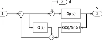
Figure 3. Disturbance observer control chart.
Figure 3 shows the block diagram of DOB, where r is the input signal of the velocity loop, d is the external disturbance of the system, Gp(s) is the transfer function of the real object, Gn(s) is the transfer function of the nominal object, and Q(s) is the low-pass filter. The real model Gp(s) can
be described by the nominal model Gn(s) and a variable transfer function D(s):
Gp(s)=Gn(s)[1+D(s)] In the transfer function, the input signal is Gcy(s), and the disturbance signal is Gdy(s). In the effect of low-frequency input signals, Q(s)≈1 gives rise to Gcy(s)≈Gn(s) and Gdy(s)≈0; Likewise in the effect of high-frequency input signals, Q(s)≈0 gives rise to Gcy(s)≈Gp(s) and Gdy(s)≈Gp(s). As the frequency band increases, the anti-interference ability of the system increases and the robustness decreases. In other words, the order, bandwidth, and relative degree of Q(s) are of prime importance to be considered in the design of DOB. The following sufficient conditions must be satisfied to obtain a stable DOB system:
| ( ) ( ) | 1, [0, );
|| ( ) ( ) || sup| ( ) ( ) | 1 Q s D s
Q s D s Q j D j
(22) The following filter is typically used in Q(s):
2 1 1
1 ( )
( )
1 ( )
N
k k k
N k k k
a s Q s
a s
(23) The relative degree of Q(s) must not be less than that of Gn(s). In this study, it suggests:
3 3 2 2
3 1 ( )
3 3 1
s Q S
s s s
(24) The use of different values can result in different cut-off frequencies of Q(s).
Simulation Verification
The Calculation of Discrete Sampling Period
variables are within |u(t)|≤u0=5, the continuous transfer function can be discretized by using the sampling period, and then the discrete feed-forward controller ZPETC is designed accordingly. With the purpose of minimizing the continuous loss function described in Eq. 10, the sampling period Tm and weight coefficient p are selected.
2 160 ( )
40 160
Gc s
s s
(25) The weight coefficient p(0) for the zero sampling period can be calculated from Eq. 11:
2 160
*5
0 160 0.42
12 0
1
(0) 0.98
( 2) 0.42 * (2 0.42)
Ku m
y
K p
m m
(26)
The controllable canonical form of closed-loop transfer function Gc(s) can be expressed as:
x Ax Bx y Cx
(27) Where
40 160 1
0 160
1 0 0
A B C
(28) Then, the loss function can be transformed into:
2
0 ( (0) )
T
J
x Qx p u dt(29) Where
0 0 0
[0 160]
160 0 25600
T
Q C C
(30)
The minimal loss of the continuous optimal controller is:
(0) (8.7 386.6)
L (31) The approximate reference sampling period Tm can be calculated from Eq. 14:
2 2 160
1.3 0.004
0.64 8.7 160 *386.6
m
T
(32) The sampling period and weight coefficient can be determined from Eq. 18:
0 0.5* 0.002 0.4 (0) 0.394
m
T T
p p
(33)
Design of ZPETC
Discrete Sampling Period. The transfer function Gc(s) can be discretized using zero-order holder, and its sampling period is T0=0.002s, by which the following discrete transfer function Gc(z) can be obtained:
1 1
1 2
(0.001558 0.001517 ) ( )
1 1.922 0.9246 c
z z
G z
z z
1 2
2
1 2 2
*(1 1.961 0.9608 )*(0.001558 0.001517 ) ( )
(0.001558 0.001517) ( ) (1 1.961 0.9608 )*(164.77 160.4 ) z
z
z z z z
G z
G z z z z z
(35)
Discrete Sampling Period. When the sampling period is T0=0.001s, the discrete transfer function Gc(z) is:
1 1
1 2
(0.0003937 0.0003895 ) ( )
1 1.961 0.9608
c
z z
G z
z z
(36) Then, the feed-forward controller ZPETC can be designed:
1 2 2
( ) (1 1.961 0.9608 )*(641.8 633.3 ) z
G z z z z z
(37)
Simulation and Analysis
The parameters are as follows, Gc(s)=160/(s2+40s-160), kp=5, =0.002, T0=0.002s, and y(t)=5sin(2*t). The simulation results based on the ZPETC and DOB designed in this project are shown in Figure 4-Figure 7. It shows the optimal value of T0 of the feed-forward controller ZPETC is 0.002s with excellent position tracking performance and contour error precision in Figure4 and Figure 5. On the contrary, the system output are divergent with other values of T0 as shown in Figure 6 and Figure 7. Thus, the method presented in this project is valuable and effective to determine the optimal discrete sampling period, and thereby, to design an optimal discrete controller.
[image:7.612.341.452.353.441.2]
Figure 4. Position tracking curves. Figure 5. Position following error curves.
[image:7.612.343.448.475.558.2]
Figure 6. Position tracking curves. Figure 7. Position tracking curves.
Conclusions
The optimal discrete sampling period was determined by balancing the offset loss and the control loss, and then a ZPETC was designed via adding DOB to enhance the anti-interference ability and robustness of the system. The proposed methods are capable of improving the stability and velocity of the discrete controller, and reducing the contour error of the system. This results may be of importance for various trajectory tracking applications.
Acknowledgment
This work was supported by the Science and Technology Program of Guangdong Province under grand number 2015B010114004.
T0=0.002s
T0=0.001s
T0=0.002s
References
[1] Ximei Z., Qingding G., Robust Tracking Control Based on ZPETC and DOB for Permanent Magnet Linear Synchronous Motor, C. Proceedings of the CSEE, 30(2007)60-63.
[2] Xiaodong L., Yunjie W., Youmin L A O A, et al, Digital Servo Control Based on Adaptive Zero Phase Error Tracking Controller & Zero Phase Prefilter, C. Chinese Control & Decision Conference, (2010)3492-3497.
[3] Xinglin C., Chuan L., Naixin Z., et al, Controller design based on ZPETC-FF and DOB for precision motion platform, J. Journal of harbin institute of technology, 46(1)(2014)1-6
[4] Zhonghua D., Naisheng Z., Shanmei C., et al, Zero phase error tracking control for AC position servo control system, J. Transactions of china electrotechical society, 6(1998)14-17.
[5] Zhijun L., Chengying L., Fanwei M., et al, ZPETC and DOB based controller design for PMLSM and experimental investigation, C. Proceedings of the CSEE, 32(2012)134-140.
[6] Adnan R., Ismail H., Ishak N., et al, Real-time adaptive feedforward Zero Phase Error Tracking Control for X-Y motion, C. IEEE International Conference on System Engineering & Technology, (2012)1-6.
[7] Barton K.L., Alleyne A.G., A Cross-Coupled Iterative Learning Control Design for Precision Motion Control, J. IEEE Transactions on Control Systems Technology, 16(6)(2008)1218-1231. [8] Hsu, Syh-Shiuh Yeh, Pau-Lo, Estimation of the contouring error vector for the cross-coupled control design, J. IEEE/ASME Transactions on Mechatronics, 7(1)(2002)44-51.
[9] Ouyang P.R., Dam T., Pano V., Cross-coupled PID control in position domain for contour tracking, J. Robotica, 33 (6)(2015)1351-1374.
[10] Su K., Cheng M., Chang Y., Contouring accuracy improvement of parametric free-form curves -A Fuzzy Logic-based Disturbance Compensation approach, C. IEEE International Conference on Mechatronics. 6(2013)730-735.
[11] Masayoshi Tomizuka, Zero Phase Error Tracking Algorithm For Digital Control, J. American Society of Mechanical Engineers, Dynamic Systems and Control Division, 109(1)(1985)65-68. [12] Wei Huang, Xin Wang, Tracking rover simulator attitude control Based on Zero Phase Error, J. Servo Control, 2(2013)37-40.
[13] Li Zhou, Shihong Yang, Xiaodong Gao, Gain-characteri-stics manipulation technique for zero phase error tracking controller, J. Control Theory & Applications. 5(2012)655-659.
[14] Chunhong Zhang, Qiang Liu, Tracing experiment study on zero phase error linear motor servo system based on interpolation compensation, J. Machine Tool & Hydraulics. 7(2011)18-20.