Two stages optimization model on make or buy analysis and quality improvement considering learning and forgetting curve

(1)

https://doi.org/10.3926/jiem.2615

Two Stages Optimization Model on Make or Buy Analysis and Quality

Improvement Considering Learning and Forgetting Curve

Mega Aria Pratama , Cucuk Nur Rosyidi , Eko Pujiyanto Universitas Sebelas Maret Surakarta (Indonesia)

[email protected], [email protected], [email protected]

Received: March 2018 Accepted: July 2018

Abstract:

Purpose: The aim of this research is to develop two stages optimization model on make or buy analysis and quality improvement considering learning and forgetting curve. The first stage model is developed to determine the optimal selection of process/suppliers and the component allocation to the selected process/suppliers. The second stage model deals with quality improvement efforts to determine the optimal investment to maximize Return on Investment (ROI) by taking into consideration the learning and forgetting curve.

Design/methodology/approach: The research used system modeling approach by mathematically modeling a system which consists of a manufacturer with multi suppliers where the manufacturer tries to determine the best combination of their own processes and suppliers to minimize certain costs and provides funding for quality improvement efforts for their own processes and suppliers.

Findings:This research provides better decisions in make or buy analysis and to improve the components by quality investment considering learning and forgetting curve.

Research limitations/implications: This research has limitations concerning investment fund that assumed to be provided by the manufacturer which in the real system the fund may be provided by the suppliers. In this model, we also do not differentiate between two types of learning, namely autonomous and induced learning.

Practical implications: This model can be used by a manufacturer to gain deeper insight in making decisions concerning process/suppliers selection along with component allocation and how to improve the component by investment allocation to maximize ROI.

Originality/value: This paper combines two models, which in previous research both models are discussed separately. The inclusion of learning and forgetting also gives a new perspective in quality investment decision.

Keywords: quality improvement, quality investment, learning and forgetting curve, return on investment

To cite this article:

(2)

1. Introduction

In a tight market competition, a manufacturing company must formulate the best strategy to win the competition. According to Mustajib and Irianto (2010), a manufacturing company has to produce not only a good product at a competitive price, but also on-time delivery and fast service to satisfy the customers. But, it becomes a challenge for manufacturing company to fulfill those requirements by improving their production eficiency. Greater eficiency will make a manufacturing company produces their product at lower cost and will get better revenue without compromising the quality (Kumar & Sosnoski, 2009).

Generally, a manufacturing company will use their own resources to produce their needed component for final product assembly. It is known as in-house production. By use in-house production method, manufacturing company can maximize the utilization of their production facilities and get better control of the quality and cost. Unfortunatelly by the growth of the market, a manufacturing company is often constrained by their capacities and capabilities to fulfill the market demand. So, to overcome this problem, they usually use an instant solution called outsourcing. According to Belcourt (2006), manufacturing companies were triggered to an outsourcing option since many outsourcing companies provide services on workers, machines or even production activities. But, outsourcing decision is not an easy task. Suppliers have many uncertainties in terms of cost, quality and delivery (Teeravaraprug, 2008). Manufacturing company has to choose the suppliers that meet their standard of performance.

After manufacturing company selects the appropriate suppliers, there is another problem that follows about how to allocate the components to the selected prcesses and suppliers. Rosyidi, Pratama, Jauhari, Suhardi and Hamada (2016) developed a make or buy analysis model to solve the above problems. In the model, a manufacturing company will be able not only to choose the best alternative that give the minimal cost, but also the allocation for each choosen alternative. The objective function of the model is to minimize the total cost which consists of manufacturing cost, purchasing cost, quality loss, scrap cost, and lateness cost. The manufacturing cost is resulted from the total cost of in-house production activities, while purchasing cost from the total cost of outsourcing activities. Quality loss dealt with the customer quality cost, while scrap cost dealt with the cost from discarding the component which did not conform to the specifications. Lateness cost is the penalty cost for company if they pass the due date to deliver the product to their customer (Rosyidi, Fatmawati & Jauhari, 2016). The model also considered several constraints such as capacity constraint, demand constraint, selected process constraint, stock removal constraint, process sequencing constraint and binary constraint.

After manufacturing company makes decision about make or buy and its allocation, they have to maintain or even improve their product quality through quality improvement both in-house and supplier sides. Quality improvement can be done in a manufacturing company by investing some fund to their processes in order to reduce the variance of their final product. The manufacturing company has to know exactly about what kind of investment they have to make. There are some kinds of investments that can be adopted by manufacturing company. The first is technology (machine) investment. According to Dunne, Foster, Haltiwanger and Troske (2004), by investing a new machine or technology, manufacturing company will improve their product quality, productivity, and revenue. The second is human resource investment. According to Blundel, Dearden, Meghir and Sianesi (1999), human resource investment included training, workshop, recruitment etc. In this paper, learning investment is considered to improve product quality by reducing product variance (Moskowitz, Plante & Tang, 2001).

(3)

learning investment will maximize the Return on Investment (ROI). The amount of ROI will be used as the objective function of the Second Stage Model (SSM).

In this research, those two models above will be solved sequentially to help manufacturing company, not only to choose optimal alternatives between make or buy decision, but also the quality improvement. In practice, this research will contribute to solve the make or buy decisions along with the component allocations and also determine the optimal variance reduction to maximize the ROI.

2. Literature Review

2.1. Previous Research on Make or Buy Deisions

Make or buy problem has been attracted many researchers to determine the components that must be produced in-house or outsourced. In addition, many reseachers also have combined the make or buy problem with another topics such as tolerance design, quality loss, Analytic Hierarchy Process (AHP), etc. Chase, Greenwood, Loosli and Hauglund (1990) developed an optimization model to select a process that gives optimal component tolerance in an assembly product. The research was considered to be the earliest model in this topic. Hambali, Sapuan, Ismail and Nukman (2009) developed a model in process selection for composite manufacturing using Analytical Hierarchy Process. Mustajib and Irianto (2010) developed an integrated model for process selection and quality improvment in multi-stage process. Rosyidi, Fatmawati et al. (2016) developed a process selection model to minimize manufacturing cost, quality loss and lateness cost in a make to order manufacturing system.

Supplier selection research have also attracted many researchers. For example, Feng, Wang and Wang (2001) developed an optimization model for concurrent selection of tolerance and suppliers. Teeravaraprug (2008) developed a model for outsourcing and vendor selection based on Taguchi loss function. Rezaei and Davoodi (2008) developed a deterministic, multi-item inventory model with supplier selection and imperfect quality. Sabatini, Jauhari and Rosyidi (2011) developed a supplier selection model based on tolerance allocation to minimize purchasing cost and quality loss. Rosyidi, Murtisari and Jauhari (2016) developed a concurrent optimization model for supplier’s selection, tolerance and component allocation with fuzzy quality loss.

Furthermore, the research on both process and supplier selection or make or buy problem have been conducted by following reseachers. Bajec and Jakomin (2010) discussed about the importance of make or buy decisions for a company. Rosyidi, Akbar and Jauhari (2014) developed a make or buy analysis model on tolerance design to minimize manufacturing cost and quality loss. The research was based on previous models developed by Chase et al. (1990) and Feng et al. (2001). Rosyidi, Pratama, Jauhari, Suhardi and Hamada (2015) and Rosyidi, Puspitoningrum, Jauhari, Suhardi and Hamada (2016) developed a make or buy analysis model with multi-stage manufacturing process to minimize manufacturing cost and taguchi quality loss (2015) and also fuzzy quality loss (2016). Pratama and Rosyidi (2017) developed a make or buy decision model with multi-stage manufacturing process and supplier imperfect quality. Rosyidi, Pratama et al (2016) developed a make or buy analysis model in a multi-stage manufacturing processes. The model will become a basis for this research as the first stage model. The output of this model will become the input for the second stage model of this research.

2.2. Previous Research on Quality Improvement with Learning and Forgetting Curve

(4)

In quality improvement studies, the role of learning curve can not be ignored. Actually, learning curve has been used in many fields. For example, Womer (1979) developed a model about learning curves, production rate, and program cost. Cunningham (1980) used the learning curve as a management tool. Fine (1986) studied about quality improvement and learning curve in a productive system. Moskowitz et al. (2001) developed a model on allocation of quality improvement targets based on investments in learning. Serel, Dada, Moskowitz and Plante (2002) conducted a research about quality investment under autonomous and induced learning. Rosyidi, Jauhari, Suhardi and Hamada (2016) developed a variation reduction model for quality improvement to minimize investment and quality costs by considering suppliers’ learning curve. Later, Rosyidi, Nugroho, Jauhari, Suhardi and Hamada (2016) developed an optimization model about quality improvement through variance reduction of component by investment allocation in learning.

The applications of learning curve in those researches above have not been considered forgetting curve in the model. To find a better result, we have to include not only learning curve but also forgetting curve. Learning and forgetting curves have been used in various fields of research. Li and Cheng (1994) developed a model of economic production quantity by considering learning and forgetting aspects. Jaber and Bonney (1997) conducted a study of the relationship between learning curve and forgetting curve. Jaber and Bonney (2003) developed a lot sizing model considering learning and forgetting aspects to improve product quality. Badiru (1995) conducted a multivariate analysis of learning and forgetting effects on product quality. This research, especially the SSM will develop based on learning and forgetting curves.

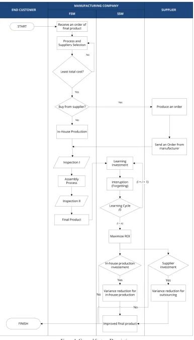
3. Model Development

3.1. System Description

In this research, we develop two models, namely First Stage Model (FSM) and Second Stage Model (SSM). The output of FSM will become the input for SSM. FSM is an optimization model in make or buy analysis to select an alternative between in-house, outsource, or both. This model also determines the component allocation for every decision. Once the number of components are determined, those components will be inspected to ensure their quality and will be assembled into the finished product. Based on the results of the allocation, the variance of every single component is known which will be used as the input of SSM.

(5)

(6)

3.2. Model Formulation 3.2.1. Notations

QL : Current Quality Loss Cost Q*

L : Quality loss cost after the learning and forgetting L*

cik : Optimal learning investment

m : Machine index

k : Component index

σ2

Ri** : Variance after the learning and forgetting d0 : Current memories

b(t) : Interruption time l *

ik : Optimal Learning rate g(t) : Learning Periods LCik : Learning investement lik : Learning rate

Pik : Proportion of variance reduction LCik Max : Maximum fund in cycle i

LC(i – 1)k Max : Maximum fund in cycle i-1 LC *

(i – 1)k : Optimal learning investment in cycle i – 1

j : Supplier index

χk : Component allocation from selected alternative I : Learning cycle index

A : Quality Loss Cost Coefficient σ2

Ri : Assembly product variance di : Residual Memories after forgetting fi : Forgetting rate

σ2

ik* : Component variance after learning

Ie : Cost coefficient for the exponential investment function LC *

ik :Optimal learning rate for each component and cycle

3.2.2. Objective Function

(7)

(2) The next cost considered in the objective function is quality loss after the occurrence of learning and forgetting. Before formulating this cost, first we have to find the component variance after learning and forgetting. Quality loss after the occurrence of learning and forgetting is formulated in Equation (3).

(3) Component variance after the occurrence of learning and forgetting can be obtained by calculating residual memories after forgetting occurs in every cycle as formulated in Equation (4).

(4) Then, component variance after the occurrence of learning and forgetting can be obtained by Equation (5).

(5) Assembly variance after the occurrence of learning and forgetting is formulated in Equation (3) and can be obtained with Equation (6).

(6) Component variance after the learning process is formulated in Equation (7).

(7)

Optimal learning rate for each component and cycle are obtained from Equation (8).

(8)

Cost coefficient for the exponential investment function is formulated in Equation (9) below.

(9) Learning investment for each component and cycle obtained from the following equation below.

(10)

Proportion of variance reduction (pik) in Equation (10) is the decision variable in the SSM. Learning rate for each component and cycle can be obtained by following equation.

(11) The optimal learning investment can be found by considering optimal learning rate in Equation (8) and Learning investment in Equation (10). Equation (12) shows the formula.

(8)

In every learning cycle, there will be a maximum investment fund. The maximum fund for cycle i can be obtained by determining the difference between maximum found at cycle i – 1with optimal learning investment at cycle i – 1 for each component. Equation (13) shows the formula. Equation (13) shows the formula.

(13) Based on the calculation of each cost above, then the return on investment can be calculated as in Equation (14).

(14)

3.2.3. Model Constraints

This SSM considers two constraints, namely learning investment and learning rate constraints. Learning rate constraint is used to ensure that the maximum fund provided by the company is greater than learning investment cost for each component. Equation (15) shows this constraint formula.

(15) Optimal learning rate constraint is used to ensure that the company will get further variance reduction. To meet this requirement, the optimal learning rate must be equal or greater than the current learning rate. Equation (16) shows this constraint formula.

(16)

4. Numerical Example

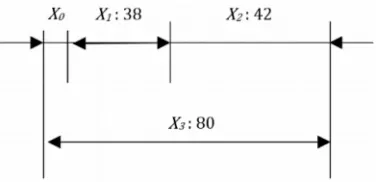
A numerical example is used in this research to show how the model works in a case. The example in this research refers to the case in Cao, Mao, Ching and Yang (2009) with some adjustments of the parameters to fit the model. In this research, the product consists of three components: Revolution axis, End shied nut and Sleeve. Figure 2 shows the dimensional chain of the assembly. The dimension of the revolution axis (x1), end shield nut (x2), and sleeve

(x3) are 38 mm, 42 mm, and 80 mm, respectively. To maintain good performance, a gap of x0 (the important quality

characteristic) with a tolerance of 0.2 mm is required.

In this numerical example, it is assumed that the manufacturing company has two stages of the production process (cell) used to produce the three components. Each stage of the process has three identical machines. Each machine and supplier have different characteristics in term of manufacturing costs, processing time and tolerance. Table 1. shows the machine characteristics in cell 1, whereas Table 2. shows the machine characteristics in cell 2. Table 3. shows the characteristics of each supplier. Table 4. shows the machine's production capacity and supplier capacity and Table 5. shows the sequence of processes for each component.

(9)

Figure 2. The dimensional chain

Cell 1

Component

Machine 1 Machine 2 Machine 3

Tol.

(mm) (IDR)Cost

Proc. time

(Min) (mm)Tol. (IDR)Cost

Proc. time

Proc. Time (Min)

1 0.008 40,000 9 0.005 50,000 14 0.003 60,000 13

2 0.008 45,000 10 0.005 57,500 15 0.003 65,000 14

3 0.008 60,000 12 0.005 65,000 18 0.003 75,000 16

Table 1. Machine characteristics in Cell 1

Cell 2

Component

Machine 1 Machine 2 Machine 3

Tol.

Proc. time

Proc. Time (Min)

1 0.006 55,000 12 0.0045 60,000 9 0.007 40,000 15

2 0.006 67,500 14 0.0045 70,000 9 0.007 45,000 16

3 0.006 75,000 17 0.0045 80,000 10 0.007 50,000 18

Table 2. Machine characteristics in Cell 2

Component

Supplier 1 Supplier 2

Tolerance

Processing time

(Min/Unit) Tolerance(mm) (IDR)Cost

Processing time (Min/Unit)

1 0.005 75,000 25 0.025 70,000 20

2 0.005 80,000 32 0.025 72,500 24

3 0.005 87,500 35 0.025 77,500 31

Table 3. Suppliers characteristics

Cell 1 Cell 2

Supplier 1 Supplier 2 Machine 1 Machine 2 Machine 3 Machine 1 Machine 2 Machine 3

800 800 800 800 800 800 800 700

(10)

The FSM is solved using oracle crystal ball software. The algorithm used for the optimal solution search in Oracle Crystal Ball is the combination between tabu search and scatter search (Oracle Corporation, 2008). The results of the optimization are shown in Table 6.

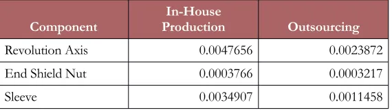
From Table 6, we can see that to meet the 1,000 units demand, the company must produce 450 units of Component 1 on Machine 2 in Cell 1 followed by 450 units on Machine 1 on Cell 2, and the remaining number of Component 1 must becprovided by Supplier 1. While for component 2, 240 units will be produced on Machine 3 at Cell 1 followed by Machine 3 at Cell 2, and the remaining number of Component 2 must be supplied by Supplier 1 and Supplier 2 for 160 and 600 units respectively. 300 units of Component 3 produced on Machine 2 and 200 units on Machine 3 in Cell 1, followed by Machine 1 and Machine 3 on Cell 2 with the same component quantities. The remaining components will be supplied by Supplier 1 and Supplier 2 for 260 and 240 units respectively. The total cost resulted from the optimization is IDR. 307,711,391. The manufacturing cost, purchasing cost, external quality loss, scrap cost, and lateness cost are IDR. 140,050,000 IDR. 138,900,000 IDR. 25,825,846, and IDR. 2,185,545 and IDR. 750,000 respectively. From this optimization result, we can determine each component variance that will be improved using the SSM. Table 7 shows the current variance from both in-house and outsourcing result.

The company has to continuously improve the component quality by reducing the component variance either in-house production or outsourcing. It aims to get better quality of the final product. The company has to invest some funds in the form of learning investment for each component. The investment allocation for each component is IDR. 25,000,000 for in-house process and IDR. 10,000,000 for suppliers. In this numerical example, we assume there are four learning cycles (i = 4), in which each cycle consists of 4 learning periods (g (t) = 4). In every learning cycle there are some interruption time. In this numerical example, the interruption time is assumed to be 3 periods (b(t) = 3). The forgetting rate (fi) is assumed to have different value of 0.08, 0.06, 0.04 and 0.02 at each cycle. In addition, the operator memories of the learning process just before the break time is assumed to be 100% (d0 = 100%). The company has spent the previous year's investment of IDR. 500,000 for each component and establishes the quality loss cost coefficient for the final product of IDR. 2,000,000.

Component 1 Cell 1 → Cell 2

Table 5. Process sequence of the components

Component

Cell 1 Cell 2

Supplier 1 Supplier 2

M 1 M 2 M 3 M 1 M 2 M 3

1 – 450 – 450 – – 550 –

2 – – 240 – – 240 160 600

3 – 300 200 300 – 200 260 240

Table 6. First stage optimization results

Component ProductionIn-House Outsourcing

Revolution Axis 0.0047656 0.0023872

End Shield Nut 0.0003766 0.0003217

Sleeve 0.0034907 0.0011458

(11)

The objective of SSM is to determine the optimal variance reduction based on the allocation of components from each selected machines and or suppliers by maximizing Return on Investment at the end of the fourth cycle of the learning investment by considering the forgetting factor. The optimization process in this second stage model also uses the same algorithm with the first stage model and it is processed using Oracle Crystal Ball software. The results of optimization are shown in Tables 8-11.

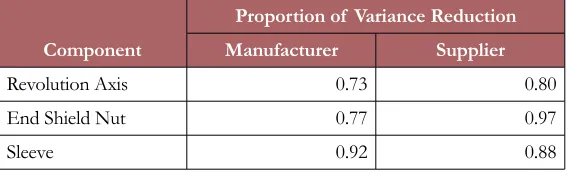
Based on the proportion of variance reduction in the tables above, the component variance can be reduced from both the manufacturer and the supplier. The results of variance reduction are shown in Tables 12 and 13.

Component

Proportion of Variance Reduction Manufacturer Supplier

End Shield Nut 0.79 0.92

Sleeve 0.96 0.86

Table 8. Proportion of Variance Reduction at first cycle

Component

Sleeve 0.92 0.88

Table 9. Proportion of Variance Reduction at second cycle

Component

Sleeve 0.91 0.77

Table 10. Proportion of Variance Reduction at third cycle

Component

Sleeve 0.79 0.57

Table 11. Proportion of Variance Reduction in fourth cycle

Component

Variance _{Percentage of}

Variance Reduction Early 1st_cycle _{End 4}th_Cycle

Revolution Axis 0.0047656 0.0030371 36.27%

End Shield Nut 0.0003766 0.0002928 22.26%

Sleeve 0.0034907 0.0026591 23.83%

(12)

Component

Variance _{Percentage of}

Variance Reduction Early 1st_cycle _{End 4}th_Cycle

Revolution Axis 0.0023872 0.0008919 62.64%

End Shield Nut 0.0007469 0.0002502 66.50%

Sleeve 0.0011458 0.0004602 59.83%

Table 13. Variance Reduction in supplier side

Component

Quality Loss Cost

Early 1st_cycle _{End 4}th_Cycle

Revolution Axis IDR. 15,539,380 IDR. 6,394,061

End Shield Nut IDR. 8,287,670 IDR. 3,410,166

Sleeve IDR. 17,265,978 IDR. 7,104,512

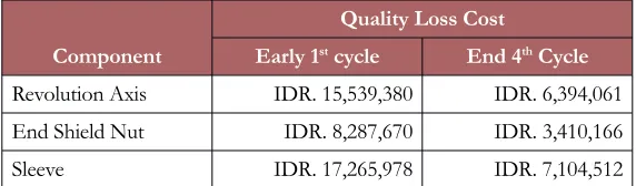
Table 14. Reduction of quality loss in manufacturer side

Component

Revolution Axis IDR. 4,707,927 IDR. 1,762,561 End Shield Nut IDR. 6,505,500 IDR. 2,435,540

Sleeve IDR. 4,279,934 IDR. 1,602,329

Table 15. Reduction of quality loss in supplier side

Component

Revolution Axis IDR. 20,247,308 IDR. 8,156,622

End Shield Nut IDR. 14,793,169 IDR. 5,845,705

Sleeve IDR. 21,545,912 IDR. 8,706,841

Total IDR. 56,586,389 IDR. 22,709,168

Table 16. Total reduction of quality loss

From the variance reductions obtained above, the reductions of quality loss cost from both the manufacturer and the suppliers can be determined as shown in Tables 14-16.

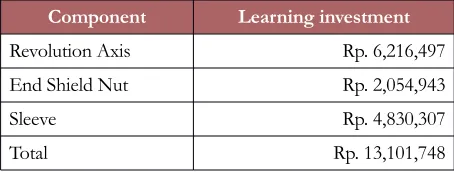
To get the variance reduction, the company must allocate some funds to a learning investment. The company make a learning investment on each component, with a maximum fund allocation of IDR.25,000,000 for the manufacturer and IDR. 10,000,000, for supplier of each component. This difference is due to companies prioritizing the reduction of variance made by the manufacturer (in-house). The allocation of funds must be managed so that it can be used to make learning investments until the end of the cycle. Tables 17-19 show the details of learning investment of each component made by the manufacturer, supplier and total learning investment.

(13)

Component Learning investment

Revolution Axis Rp. 24,455,974

End Shield Nut Rp. 4,346,588

Sleeve Rp. 5,178,073

Total Rp. 33,980,635

Table 17. Learning investment in manufacturer side

Sleeve Rp. 4,830,307

Total Rp. 13,101,748

Table 18. Learning investment in supplier side

Sleeve Rp. 10,008,380

Total Rp. 47,082,383

Table 19. Total learning investment

Component Return on Investment

Revolution Axis 37.40%

End Shield Nut 112.21%

Sleeve 196.24%

Total 71.17%

Table 20. ROI in manufacturer side

Sleeve 55.43%

Total 73.98%

Table 21.ROI in supplier side

Sleeve 128.28%

Total 71.95%

(14)

We also compare the SSM in this paper with the model of Rosyidi, Nugroho et al. (2016). The main difference between those two models is the existence of forgetting curve in SSM which was not considered yet in Rosyidi, Nugroho et al. (2016). The results of the optimization in term of quality loss and learning investment are shown in Table 23. From the table we can see that the SSM gives lower quality loss both current and after variance reduction. The difference between both total costs are IDR.77,925,275 and IDR. 51,923,693 for SSM and Rosyidi, Nugroho et al. (2016) respectively. The costs show that the SSM performs better in quality improvement than Rosyidi, Nugroho et al. (2016). The better improvement in quality loss of the SSM needs 77.4% higher learning investment than Rosyidi, Nugroho et al. (2016). This result shows that by incorporating forgetting curve in the model gives better results in quality loss with the consequnces of higher learning investment. The learning investment is justified due to the savings gain by the company in term of quality loss.

Component

SSM

(IDR) Rosyidi, Nugroho et al. (2016)(IDR)

Current QL ReductionAfter Var. InvestmentLearning Current QL ReductionAfter Var. InvestmentLearning Revolution Axis 39,559,005 11,419,441 33,725,100 136,611,737 117,659,593 18,661,279 End Shield Nut 28,293,495 8,676,541 29,346,420 98,987,643 86,510,010 11,485,395

Sleeve 42,241,270 12,072,513 26,563,936 145,569,855 125,076,160 20,379,749

Total 110,093,770 32,168,495 89,635,456 381,169,235 329,245,763 50,526,423

Table 23. Results of model comparison

5. Sensitivity Analysis

Sensitivity analysis is used to study the effect of the parameters in the model to both decision variables and objective function (Daellenbach & McNickle, 2005). This analysis will be focused to the SSM. There are two scenarios in this sensitivity analysis. The first scenario is performed by changing the interruption time (b(t)) and the learning cycle (i). Table 24 shows the scenarios.

b(t ) (Periods) 2 3 4 5

i (Cycle) 1 2 3 4

Table 24. Scenarios of sensitivity analysis

5.1. Interruption Time (b(t)) Effects

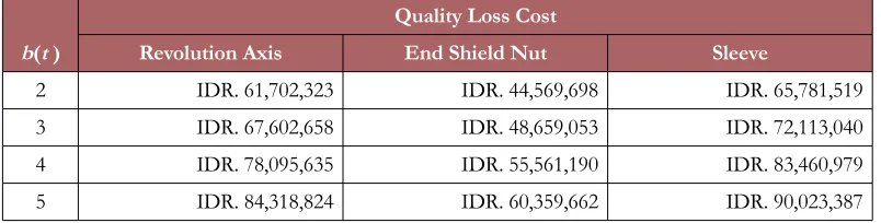
Interruption time indicates how long a worker will experience the forgetting process. The occurrence of long interruption will have a negative impact to the manufacturing company. In addition, an increase of the interruption time will make the variance target will not achieved. This first scenario of sensitivity analysis will show how the model behaves to the change of parameters. The b(t) value used in this scenarios are 2, 3, 4 and 5 periods. The changes in b(t) affects the amount of quality loss. Table 25 shows the influence of interruption time to the quality loss.

(15)

b(t )

Revolution Axis End Shield Nut Sleeve

2 IDR. 61,702,323 IDR. 44,569,698 IDR. 65,781,519

3 IDR. 67,602,658 IDR. 48,659,053 IDR. 72,113,040

4 IDR. 78,095,635 IDR. 55,561,190 IDR. 83,460,979

5 IDR. 84,318,824 IDR. 60,359,662 IDR. 90,023,387

Table 25. Effects of interruption time to the quality loss

b(t )

Variance Reduction Percentage

Revolution Axis End Shield Nut Sleeve Total

2 51.96% 43.57% 47.12% 47.55%

3 41.27% 42.54% 36.77% 40.19%

4 19.83% 26.42% 21.71% 22.65%

5 11.17% 10.31% 2.72% 8.07%

Table 26. Effects of Interruption time to the variance reduction

b(t )

Return on Investment

2 132.45% 84.66% 114.92% 110.17%

3 54.95% 41.93% 67.38% 54.46%

4 45.80% 26.25% 41.39% 3720%

5 25.22% 17.54% 18.14% 19.96%

Table 27. Effects of Interruption time to the ROI

In addition to the effect on the cost of quality loss, the changes in interruption time (b(t)) will also affect the variance reduction percentage obtained by the company. Table 26 shows the effect of changes of b(t) on the variance reduction percentage.

From Table 26, we can see that each value of b(t) will increase, while the variance reduction percentage will decrease. For example, when the value of b(t) is 4 periods, the variance reduction percentage for the Revolution Axis is 19.83%, and when the value b(t) increases to 5 periods, the variance reduction percentage at that component decreases to 11.17%. The similar results are obtained for all other components. This occurs because the addition of the interruption time (b(t)) will increase the variance in which the greater the decrease of the variance, the lower the reducttion percentage. The change of interruption time will also affect to the ROI. Table 27 shows the effect of b(t) changes on the ROI.

(16)

Figure 3. Effects of interruption time to variance reduction

Figure 4. Effects of interruption time to The ROI

5.2. Learning cycle (i ) analysis

The learning cycle (i) is one of the important parameters considered in this model. The learning cycle is useful to give a break to a learning process in every cycle, so the forgetting process will occur. The number of learning cycles used will depend on the decision of the manufacturing company. The number of learning cycles can be determined in advanced at the beginning of the cycle and will stop when the variance reduction target has been achieved.

i

Quality Loss Costs

Revolution Axis End Shield Nut Sleeve

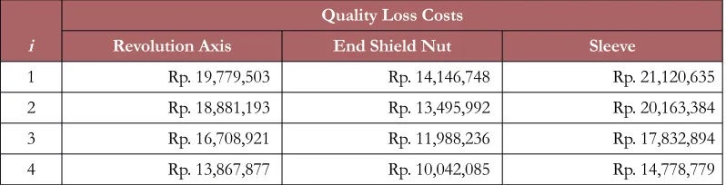
1 Rp. 19,779,503 Rp. 14,146,748 Rp. 21,120,635

2 Rp. 18,881,193 Rp. 13,495,992 Rp. 20,163,384

3 Rp. 16,708,921 Rp. 11,988,236 Rp. 17,832,894

4 Rp. 13,867,877 Rp. 10,042,085 Rp. 14,778,779

Table 28. Effects of learning cycles to quality loss

i

Variance Reduction Percentage

1 5.78% 1.13% 3.64% 5.78%

2 14.11% 5.49% 17.99% 14.11%

3 30.39% 29.35% 27.90% 30.39%

(17)

In this scenario, the learning cycle parameters (i) are assumed to be to 1, 2, 3, and 4 cycles. The addition of the learning cycle affects the quality loss as shown in Table 28.

From Table 28 above we can see that each addition of i will decrease the quality loss. When total cycle is 3, the quality loss for Revolution Axis component is IDR. 16,708,921, and when the cycle increases to 4, the value of quality loss on that component decreases to IDR. 13,867,877. Similar patterns are found for all other components. This occurs because the more learning cycles are used, the value of the variance of the product will continue to reducing. The addition of the learning cycles used also affects to variance reduction percentage. Table 29 shows the influence of learning cycles to variance reduction percentage.

From Table 29 above it can be seen that each addition of the learning cycles (i) makes the variance reduction percentage increasing. For example, when the number of i is 3 cycle, the variance reduction percentage for Revolution Axis component is 30.39%, and when the value of i is added to 4 cycle, the variance reduction percentage on that component increases to 42.08%. Similarly for all other components. This happens because the more learning cycles are used, the value of the variance of the product will continue to reduce. Of course, the variance reduction percentage will be greater.

As the objective function of this second stage model to maximize the return on investment, this change of learning cycle also affects the ROI. Table 30 shows the effect of i on the ROI.

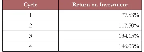
From Table 30 above we can see that the addition of the number of learning cycles (i) will increase the ROI. The resulting ROI is the accumulated ROI value of the n-cycle. For example, with 4 learning cycles, the ROI is 146.03%. The value is the accumulation of ROI from the first cycle until the fourth cycle. The increased of ROI comes from the greater variance reduction percentage, even though in the same time there will be an increase in the learning investment cost. Figure 5 shows the influence of learning cycle to the variance reduction percentage while the influence of learning cycle on the ROI is shown in Figure 6.

Cycle Return on Investment

1 77.53%

2 117.50%

3 134.15%

4 146.03%

Table 30. Effects of learning cycle to the ROI

Figure 5. Effect of learning cycle to the Variance Reduction Figure 6. Effects of learning cycle to the ROI

6. Conclusions

(18)

determine the optimal investment of quality improvement to maximize the ROI considering learning and forgetting curve. The SSM in this research gave better results compared with the previous model without forgetting curve. The SSM gave higher benefit in term of quality improvement with a consequence that the company has to spend higher learning investment. Hence the SSM is suitable for a company which has a production cycle with some learning and forgetting in the cycle and needs to continuously perform quality improvement by investment in learning. From the results of sensivity analysis, the model is quite sensitive to the parameters of the model. The increase of the interruption time will reduce the amount of ROI. More learning cycle will also increase the amount of ROI. Hence, before a manufacturing company uses this model, a careful data collection and processing must be done. For the future research, this study can be extended by differentiate between induced and autonomous learning. Moreover, this research can also be extended by using dynamic forgetting rate.

Declaration of Conflicting Interests

The authors declared no potential conflicts of interest with respect to the research, authorship, and/or publication of this article.

Funding

This research was funded by Research Grant from The Institute of Research and Community Services Universitas Sebelas Maret Surakarta under Graduate Scheme with Contract Number 543/UN27.21/PP/2018.

References

Badiru, A.B.(1995). Multivariate analysis of the effect of learning and forgetting on product quality. International Journal of Production Research, 33(3), 777-794. https://doi.org/10.1080/00207549508930179

Bajec, P., & Jakomin, I.A. (2010). Make-or-buy decision process for outsurcing. Distribution Logistics Review, 22(4), 285-291.

Belcourt, M. (2006). Outsourcing–The benefits and risks. Human Resource Management Review, 16(2), 269-279. https://doi.org/10.1016/j.hrmr.2006.03.011

Bernstein F., & Kok, A.G. (2009). Dynamic cost reduction through process improvement in assembly networks. Management Science, 55(4), 552-567. https://doi.org/10.1287/mnsc.1080.0961

Blundell, R., Dearden, L. Meghir, C., & Sianesi, B. (1999). Human capital investment: The returns from education and training to the individual, the firm and the economy. Fiscal Studies, 20(1), 1-23.

https://doi.org/10.1111/j.1475-5890.1999.tb00001.x

Cao, Y., Mao, J., Ching, H., & Yang, J. (2009). A robust tolerance optimization method based on fuzzy quality loss. Proceedings of the Institution of Mechanical Engineers Part C: Journal of Mechanical Engineering Science, 223(11), 2647-2653. https://doi.org/10.1243/09544062JMES1451

Chase, K.W., Greenwood, W.H., Loosli, B.G., & Hauglund, L.F.(1990). Least cost tolerance allocation for mechanical assemblies with automated process selection. Manufacturing Review, 3(1), 49-59.

Cunningham, J.A. (1980). Using the learning curve as a management tool: The learning curve can help in preparing cost reduction programs, pricing forecasts, and product development goals. IEEE Spectrum, 17(6), 45-48. https://doi.org/10.1109/MSPEC.1980.6330359

Daellenbach, H.G., & McNickle, D.C. (2005). Management science: Decision making through systems thinking. New York, USA: Palgrave McMillan. https://doi.org/10.1007/978-0-230-80203-2

(19)

Fine, C.H. (1986). Quality improvement and learning in productive systems. Management Science, 32(10), 1301-1315. https://doi.org/10.1287/mnsc.32.10.1301

Hambali, A., Sapuan, S.M., Ismail, N., & Nukman Y. (2009). Composite manufacturing process selection using analytical hierarchy process. International Journal of Mechanical and Materials Engineering, 4(1), 49-61.

Jaber, M.Y., & Bonney, M.A. (1997). Comparative study of learning curves with forgetting. Applied Mathematical Modelling, 21(8), 523-531. https://doi.org/10.1016/S0307-904X(97)00055-3

Jaber, M.Y., & Bonney, M. (2003). Lot sizing with learning and forgettig in set-ups and product quality. International Journal of Production Economics, 83(1), 95-111. https://doi.org/10.1016/S0925-5273(02)00322-5

Kumar, S., & Sosnoski, M. (2009). Using DMAIC Six Sigma to systematically improve shopfloor production quality and costs. International Journal of Productivity and Performance Management, 58(3).

https://doi.org/10.1108/17410400910938850

Li, C.L., & Cheng, T.C.E. (1994). An Economic Production quantity model with learning and forgetting consideration. Production and Operations Management, 3(2), 118-132. https://doi.org/10.1111/j.1937-5956.1994.tb00114.x

Moskowitz, H., Plante, R., & Tang, J. (2001). Allocation of quality improvement target based on investments in learning. Naval Research Logistics, 48 8), 684-709. https://doi.org/10.1002/nav.1042

Mustajib, M.I., & Irianto, D. (2010). An integrated model for process selection and quality improvement in multi-stage processes. Journal of Advanced Manufacturing Systems, 9(1), 31-48. https://doi.org/10.1142/S0219686710001788 Oracle Corporation (2008). One-minute spotlight optquest: Finding the best solutions under uncertain conditions. Pratama, M.A., & Rosyidi, C.N. (2017). Make or buy decision model with multi-stage manufacturing process and supplier

imperfect quality. AIP Conference Proceedings, 1902(1), 020026. https://doi.org/10.1063/1.5010643

Rezaei, D. & Davoodi, M. (2008). A Deterministic, multi-item inventory model with supplier selection and imperfect quality. Applied Mathematical Modelling, 32(10), 2106-2116.

Rosyidi, C.N., Akbar, R.R., & Jauhari, W.A. (2014). Make or buy analysis model based on tolerance design to minimize manufacturing cost and quality loss. Makara Journal of Technology, 18(2), 86-90.

https://doi.org/10.7454/mst.v18i2.400

Rosyidi, C.N. Pratama, M.A., Jauhari, W.A., Suhardi, B., & Hamada, K. (2015). Make or buy decision model with multi-stage manufacturing process to minimize manufacturing cost and quality loss. IEEE International Conference on Joint 3rd International Conference in Electrical Vehicular Technology and International Conference on Electric Vehicular Technology and Industrial, Mechanical, Electrical and Chemical Engineering (ICEVT – IMECE) (189-193). https://doi.org/10.1109/ICEVTIMECE.2015.7496662

Rosyidi, C.N., Fatmawati, A., & Jauhari, W.A. (2016). An integrated optimization model for product design and production allocation in a make to order manufacturing system. International Journal of Technology, 7(5), 819-830. https://doi.org/10.14716/ijtech.v7i5.1173

Rosyidi, C.N., Jauhari, W.A., Suhardi, B., & Hamada, K. (2016). A variation reduction allocation model for quality improvement to minimize investment and quality costs by considering suppliers’ learning curve. IOP Conf. Series: Materials Science and Engineering, 114(1). https://doi.org/10.1088/1757-899X/114/1/012083

Rosyidi, C.N., Murtisari, R., & Jauhari. W.A. (2016). A concurrent optimization model for suppliers selection, tolerance and component allocation with fuzzy quality loss. Cogent Engineering, 3(1), 1222043. https://doi.org/10.1080/23311916.2016.1222043

(20)

Rosyidi, C.N., Pratama, M.A., Jauhari, W.A., Suhardi, B., & Hamada, K. (2016). Make or buy analysis model in a multi-stage manufacturing processes. Proceedings of IEEE International Conference on Industrial Engineering and Engineering Management (IEEM) (971-976). https://doi.org/10.1109/IEEM.2016.7798022

Rosyidi, C.N., Puspitoningrum, W., Jauhari, W.A., Suhardi, B., & Hamada, K. (2016). Make or buy analysis model based on tolerance allocation to minimize manufacturing cost and fuzzy quality loss. IOP Conference Series: Material Science and Engineering, 114(1). https://doi.org/10.1088/1757-899X/114/1/012082

Sabatini, N., Jauhari, W.A., & Rosyidi, C.N. (2011). Supplier selection model based on tolerance allocation to minimize purchasing cost and quality loss. Proceedings of International Seminar on Industrial Engineering and Service Science (IESS). Solo, Indonesia.

Serel, D.A., Dada, M., Moskowitz H., & Plante, R.D. (2002). Investing in quality under autonomous and induced learning. IIE Transactions., 35(6), 545-555. https://doi.org/10.1080/07408170304415

Teeravaraprug, J. (2008). Outsourcing and vendor selection model based on Taguchi loss function. Songklanakarin Journal of Science and Technology, 30(4), 523-530.

Tsou, J.C., & Chen, J.M. (2005). Case Study: Quality improvement model in a car seat assembly line. Production Planning & Control: The Management of Operations, 16(7), 681-690. https://doi.org/10.1080/09537280500249223 Womer, N.K. (1979). Learning curves, production rate and program cost. Management Science, 25 (4), 312-319.

https://doi.org/10.1287/mnsc.25.4.312

Zhu, K., Zhang, R., & Tsung, F. (2007). Pushing quality improvement along supply chains, Management Science, 53(3), 421-436. https://doi.org/10.1287/mnsc.1060.0634

Zollo, M., & Winter, S.G. (2002). Deliberate learning and the evolution of dynamic capabilities. Organization Science, 13(3), 339-351. https://doi.org/10.1287/orsc.13.3.339.2780

Journal of Industrial Engineering and Management, 2018 (www.jiem.org)

Article’s contents are provided on an Attribution-Non Commercial 4.0 Creative commons International License. Readers are allowed to copy, distribute and communicate article’s contents, provided the author’s and Journal of Industrial Engineering and