Forecasting Gold Price with Auto Regressive Integrated Moving Average Model

Issues

ISSN: 2146-4138

available at http: www.econjournals.com

International Journal of Economics and Financial Issues, 2017, 7(4), 324-329.

Forecasting Gold Price with Auto Regressive Integrated Moving

Average Model

Naliniprava Tripathy*

Indian Institute of Management Shillong, Shillong, Meghalaya, India. *Email: [email protected]

ABSTRACT

The present study forecasts the gold price of India by using auto regressive integrated moving average (ARIMA) model over a period of 25 years from July 1990 to February 2015. The study also uses mean absolute error (MAE), root mean square error, maximum absolute percentage error, maximum absolute error (Max AE), and mean absolute percentage error (MAPE) to evaluate the accuracy of the model. The result of the study suggests that ARIMA (0,1,1) is the most suitable model used for forecasting the Indian gold prices since it contains least MAPE, Max AE and MAE. The study suggests that the past 1-month gold price has a significant impact on current gold price. The result of the study are particularly important to investors, economists, market regulators and policy makers for understanding the effectiveness of gold price to take better investment decision and devise better risk management tools.

Keywords: Auto Regressive Integrated Moving Average, Gold Price, Forecasting Techniques, Multiple Regression

JEL Classifications: G1, G17, C5

1. INTRODUCTION

Gold is a precious metal and different from other assets. It

is highly liquid and responds to price changes (Ranson and Wainwright, 2005). Gold plays a unique role as a store of value and hedge risks (Taylor, 1998; Capie et al., 2005; Hammoudeh et al., 2010). It plays a distinctive role not only as financial

assets in international currency reserves but also contributing

significantly to the stabilization of international money market.

Among all the investment alternatives available in the world, gold has shown continuously better performance over the years than other conventional asset class with a CAGR of 14.5% in US Dollar (USD) terms. Gold price is regarded as world’s

economic movements and also partially as reflections of investors’ expectation. During financial crises period 2008-2009, many mineral prices have dropped 40% but global gold price has

increased on an average 6% shown opposite trends. It indicates that gold price behave differently. Most of the research studies

state that the price of gold reflects inflation expectations. Because

commodity prices can incorporate new information faster than any consumer prices (Mahdavi and Zhou, 1997). The price of gold and other assets such as stocks, bonds, oil price and foreign currency

are frequently correlated (Corti and Holliday, 2010). The increase of gold price appears to lead to fall in the price of other financial

assets. Some studies have examined that the gold is viewed as

safe heaven on stock market direction. (Baur and McDermott, 2010; Baur and Lucey, 2010; Takashi and Shigeyuki, 2012). This

implies that change in gold price may be monitored by observing the movements of stock prices. Gold is an investment asset and used as a risk management tool in hedging. Investors invest in

gold to minimizing their potential losses. Hence, prediction of gold price is a vital issues in financial economics today.

Accurate forecasting of the gold price will not only help to monetary policymakers but also to hedge fund managers, and international portfolio managers to take better investment

decisions in the market. However, there is little research work has

been made on the prediction of gold price in India. The present research study seeks to address this gap. In this context, we have

raised three research questions. First, the present study will add

different forecasting performance measures such as mean absolute error (MAE), mean absolute percentage error (MAPE). Maximum absolute percentage error (Max APE), maximum absolute error

(Max AE), and root mean square error (RMSE). The structure of the paper is organized as follows: Section 2 describes the literature

review, the data and methodology are presented in Section 3, and Section 4 presents the empirical results of the study. Concluding

observation is provided in the final section.

2. LITERATURE REVIEW

Gold price prediction is receiving prominent attention among

researchers today. Larry and Fabio (1996) find that the real

appreciations or depreciations of the euro and the yen against the U.S. dollar have profound effects on the price of gold in all other currencies. Further the study suggests that the primary gold producers of the world (Australia, South Africa, and Russia)

appear to have no significant influence over the world price of gold. Khaemusunun, (2009) predicts the Thai gold price by using

Multiple Regression and ARIMA model. The study has examined the impact of currencies of the United States, Australia, Canada,

Peru, Hong Kong, Japan, Germany, Italy, Singapore, Colombia, Oil Prices and Interest Rate on the gold price. The study finds

that American, Australian, Canadian, Japanese currencies are

significantly affecting the Thai gold price. The study concludes

that ARIMA (1, 1, 1) is the most suitable model for predicting Thai

gold price. Ismail et al. (2009) use multiple linear regression (MLR)

models for forecasting the gold prices. The study has taken multiple economic factors such as commodity research bureau future index,

USD/Euro foreign exchange rate, inflation rate, money supply, New York Stock Exchange Index; standard and Poor 500 index, Treasury bill and USD index. The study finds that Commodity Research Bureau future index, USD/Euro foreign exchange rate, Inflation rate, money supply are having a significant impact on gold price. The study concludes that MLR model appeared to be useful for predicting the gold price. Hammoudeh et al. (2010) shows

that gold affects the volatility of the USD/Euro exchange rate. The study concludes that there is an interdependent exist between the volatility of gold price and the exchange rate. Kuan-Min et al.

(2011) investigates the short-run and long-run inflation hedging

effectiveness of gold in the United States and Japan. The study

finds that gold return is unable to hedge against inflation in either

US or Japan during the little momentum structures.

Ai, et al. (2012) proposes an interval method to explore the

relationship between exchange rate of the Australian dollar, USD

and the gold price. The empirical evidence finds that the exchange

rate relates to the gold price both in the long-run and short-run.

Ewing and Malik (2013) find evidence of volatility transmission between gold and oil future prices. Massarrat (2013) forecast the

gold price by using the ARIMA model. The results suggest that

ARIMA (0, 1, 1) is the most suitable model for predicting the

gold price. Pung, et al. (2013) forecast the gold prices of Malaysia by using ARIMA and GARCH model. The study concludes that GARCH model is a more appropriate model than ARIMA Model for predicting the gold prices. Rebecca et al. (2014) use ARMA model

and 6-step-ahead forecast model for predicting the monthly adjusted closing price of gold. The forecasted value than compared with

original corresponding prices. The study finds that actual values fell within the forecast limits. Nicholas (2014) investigates the dynamic

relationship between gold prices, nominal and real exchange rate

changes in Australia by using error correction model. The study finds

that gold price can be used to forecasting the Australian dollar/USD exchange rate. The study concludes that Gold price information can

improve AU Dollar/USD exchange rate forecasting significantly. Hossein et al. (2014) forecast the gold price by using both parametric and nonparametric time series model. The study finds that none of

the models provide a most accurate estimate of gold price in both the short and long run. The study concludes that univariate models are however outperforming the multivariate models for forecasting

the gold price. Hossein and Abdolreza (2015) predict the gold price by using artificial neural networks (ANN) and ARIMA model. The

result shows that ANN model outperforms ARIMA model.

3. DATA AND METHODOLOGY

The study employs monthly gold price from July 1990 to February 2015. All the required information for the study has been retrieved from the Multi Commodity Exchange of India Ltd., Yahoo Finance

website, and World gold council. The demeaned continuously compounding percentage returns of gold prices are calculated by using monthly price difference of the natural logarithms,

subtracting the sample mean and multiplying by 100.

The development of ARIMA model encompasses predominantly

three steps such as identification, estimation, and diagnostic checking. Before using ARIMA model, it is important to check

the stationarity of data. So the study uses unit root test. The selection of the regression model will be made by observing the autocorrelation (AC) function (ACF) and partial ACF (PACF).

The ACF and PACF are used to find conclusive evidence of its

stationary condition. If the ACF dies off smoothly at a geometric

rate, and the PACs become zero after one lag, then a first-order autoregressive model is appropriate. Alternatively, if the AC zero

after one lag and the partial ACs declined geometrically, then a

first-order moving average process is necessary.

3.1. Model Estimation

Box-Jenkins’ ARIMA model is one of the extensively used models

for forecasting. The model uses no other independent variable, but the prediction is made only from the historical series of a variable. The next step is to identify the model. The regressor that would be chosen to form the model will be selected from the variable

lag of time of AR (p) and MA (q).

3.2. ARIMA Model

Analysts, multinational corporations, dealers in foreign exchange, exporters, importers and speculators commonly believe that past patterns provide an indication of future movement at least in the

short run. Box and Jenkins’ (1976) ARIMA model is one of the

widely used models for predicting the gold price today. The model assumes that the future values of time series have a functional relationship with current, past values and white noise. The model uses the historical value of the series for prediction. ARIMA model takes historical data and decomposes it into an Autoregressive

of the auto regressive process, d is the order of the data stationary

and q is the order of the moving average terms based on

Box-Jenkins methodology.

The ARIMA (p, d, q) can be written as

∅_p

( )

(

)

(1)

W h e r e ∅_p

_{( )}

1 .. i s t h e

autoregressive operator of order p,

θ_q

_{( )}

1 .. is the moving average operator of order; (1−B)d is the dit difference: B is backward shift operator;

and α_t is the error term at time t.

The study used the Akaike information criterion (AIC) and Schwartz Bayesian criterion for choosing alternative ARIMA model. The models with the lowest AIC and BIC is chosen for the analysis.

3.3. Diagnostic Checking 3.3.1. AC

The most traditional test to ascertain the presence or absence of auto correlated error terms is the Durbin-Watson d-statistics. If DW statistics will be around 2, there is no serial correlation. The DW statistics will fall below two if there is a positive serial correlation. If there is a negative correlation, the statistics will lie somewhat in between 2 and 4. Since there are limitations of the DW test to test for serial correlation. So two other tests of serial

correlation-the Q-statistic and the Breusch-Godfrey LM test are

preferred in most applications.

The sophisticated method of creating the stationary condition of

the residuals is to check the Ljung-Box Q statistic. Q statistical

data is often issued, as a test of whether the series is white noise. The Q statistics at lag k is a test statistics for the null that there is no AC up to order computed as

QLB T T j

k T jj

= +

−

∑ ₋

( 2) 1

2

Γ ₍₂₎

If there is no serial correlation in the residuals, the ACs and PACs at

all lags will be nearly zero, and all Q-statistics will be insignificant.

If the Q-statistics are significant at all lags, the presence of AC

found in the sample. Such result persuades to reject the null hypothesis that price returns are independent.

3.4. Multiple Regression Model

Multiple regression is made to satisfy the purpose of finding lag

factors affecting gold Price. Simple linear regression models are

used to confirm ARIMA results. In Regression model, the lagged

values of gold prices are used for prediction.

Goldprice_t = α + βGoldprice_t-1+β₁Goldprice_t-2+β₂Goldprice t-3+β3Goldpricet-4+β4Goldpricet-5 (3)

The study also used R2 _{to know how much of the variability of}

dependent variable can be explained by independent variable (s). R2 _{only considering values between 0 and 1. Value for R}2 _close to one shows a good fit of forecasting model and a value close to zero presents a poor fit.

3.5. Forecasting Evaluation Technique

The performance of the ARIMA model is evaluated by using such as MAE, RMSE, MAPE, Max AE, and MAPE.

4. EMPIRICAL ANALYSIS

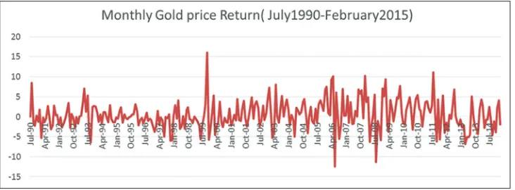
The Figure 1 exhibits the monthly gold return series. It is observed that there is an increasing trend in the performance with higher values displaying less variation in gold price return in the market.

AC is useful for finding the presence of a periodic signal. The ACF

and PACFs of the series of gold return, is presented in the Table 1.

Table 1: AC and PAC of gold return

Lag AC PAC Q-Stat P

1 0.108 0.108 3.4552 0.063

4 0.062 0.045 6.4544 0.168

8 −0.015 −0.026 7.8981 0.443

12 0.010 −0.024 20.037 0.066

16 0.082 0.073 23.187 0.109

20 0.081 0.091 28.317 0.102

24 0.044 0.046 31.326 0.145

28 0.006 0.002 32.542 0.253

32 −0.026 −0.048 33.190 0.409

36 −0.043 −0.095 38.570 0.354

AC: Auto correlation, PAC: Partial auto correlation

The ACFs and PACFs of gold price shown in Table 1, and it exhibits random walk behavior. Table 1 demonstrates that

gold price series is non-stationary and differencing. Hence, log

transformation is needed to make the series stationary. After differencing, the ACF and PACF for gold price show that the series have become stationary that depicted in Table 2.

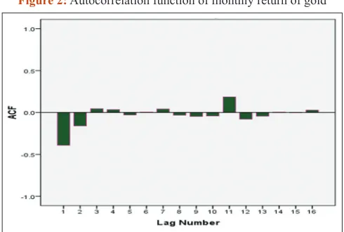
Figures 2 and 3 show the 1st _{variation of gold price series that may} have a mean of zero and distribute as white noise.

Table 2 report that Q-statistics is significant at almost all lags.

It indicates that there is an important serial correlation in the

residuals. Hence, the null hypothesis of weak-form market efficiency is rejected. It implies that relationship between the gold

returns at the current period and its value in the previous cycle

is significant. It confirms the presence of AC in the Indian gold returns and does not exhibit weak form efficiency.

Table 3 presents the Breusch-Godfrey serial correlation LM test, which is statistically significant and rejects the hypothesis. The study confirms the serial correlation. So it suggests that the

gold return does not follow Random Walks. Table 4 exhibits that Durbin-Watson statistics is within the range of 2 and indicates the

absence of first-order serial correlation.

Durbin-Watson statistical value for the model equals to 2 hence AC

problem is solved. It is observed from Table 4 that recent 1-month

gold price have a significant impact on the current gold price and

2-month lag, 3-month lag, 4-month lag and 5-month lag gold

price do not significantly affect the current month’s price pattern of gold. The `t’ value of these variables is not significant. Now it is essential to find out that whether these results are in conformity with the ARIMA findings.

As represented by the model, the multiple regression tells some information about what factors that have an impact on the gold price change. It is observed that the Indian gold prices with

one lag are significant in explaining the variation in the price

of gold.

The Table 5 shows the summary results of ARIMA model. The

BIC in Table 5 indicates that Gold price follows the ARIMA (0, 1, 1) when regressed on past gold price since the BIC value

is 6.871 which is minimum. It indicates that gold price follows

auto regressive process of order 0 and moving average process of

order 1 and differencing of 1 respectively. The analysis reveals that current gold price depends on the just preceding months'

gold price which is confirmed with our multiple regression

Table 2: AC and PAC of gold return

Lag AC PAC Q-Statistic P

1 −0.392 −0.392 45.720 0.000

4 0.034 −0.174 54.295 0.000

8 −0.033 −0.052 55.437 0.000

12 −0.080 −0.012 69.251 0.000

16 0.028 −0.037 70.114 0.000

20 0.078 0.040 75.973 0.000

24 0.038 0.024 78.019 0.000

28 0.003 0.006 81.793 0.000

32 −0.028 0.028 83.814 0.000

36 −0.066 0.003 95.831 0.000

Figure 2: Autocorrelation function of monthly return of gold

Figure 3: Partial autocorrelation function of monthly return of gold

Table 3: Breusch-Godfrey serial correlation LM test

Gold return

F-statistic 2.284695 P (F) 0.079041

Obs*R2 _{6.811276 P (Chi-square) 0.078163}

Durbin-Watson statistic 1.991123 F-statistic 1.724053

Table 4: Regression analysis of gold price on current and past gold price

Predictor

variable Coefficients Standard error t-statistic P R

2 _{Adj R}2 _{DW F P (F-statistic)}

t-1 0.122357 0.059265 2.064560 0.0399* 0.024582 0.007470 1.999435 1.436507 (0.21)

t-2 −0.081323 0.059729 −1.361535 0.1744

t-3 0.056306 0.059801 0.941549 0.3472

t-4 0.043809 0.059278 0.739033 0.4605

t-5 0.021290 0.058918 0.361357 0.7181

C 0.058918 0.213349 1.567101 0.1182

analysis. The immediate next minimum BIC is for ARIMA (1, 1, 0). These results also reinforce the findings of regression

models.

The smaller the forecasting error, better the prediction model. It is observed from the Table 6 that about 99%of the gold price is

explained by current, and past 1-month gold price. R2 _{value is} close to one shows a good fit of the forecasting model.

All RMSE, MAPE, Max APE, Max AP, and MAE are

non-negative numbers that are quite good for an ideal model. As per

RMSE, ARIMA (1, 1, 1) is the best model for forecast the gold

price. Similarly, ARIMA (1, 1, 0) and ARIMA (2, 1, 0) is also

best prediction model for gold price as per as per MAPE, Max AE and MAE model. As per MAPE, Max AE and MAE, ARIMA

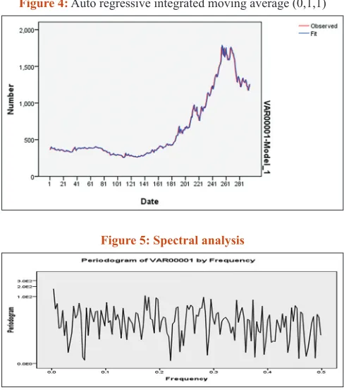
(0, 1, 1) is the best model for gold price prediction since the BIC is low and error are the least. It also confirms with our regression model. The ARIMA (0, 1, 1) selected as the best one followed by ARIMA (1, 1, 0) and ARIMA (2, 1, 0) model (Figure 4).

The study also uses spectrum analysis for predicting the value and the direction of changes in the monthly gold price. The primary

purpose of frequency analysis is to decompose the original series

into a sum of series so that each component in this amount can

identify as either a trend, periodic or quasi-periodic or noise.

Figure 5 shows a typical spectrum and an initial result is the simple

random walk model fits the data very well. The simple random walk model tells us little about the long run (low frequency)

properties of the series.

5. CONCLUSION

The present paper aim to establish and corroborate the prediction of gold price in India. The paper uses the monthly time series data to discover the forecasting of gold price. The study used ARIMA model to predict the gold price. The study has further used different

Figure 4: Auto regressive integrated moving average (0,1,1)

Figure 5: Spectral analysis

Table 6: Forecasting accuracy

ARIMA (p, d, q) RMSE MAPE Max APE MAE Max AE R2 _Rank

ARIMA (0, 1, 1) 30.459 2.702 15.316 19.010 175.355 0.995 1

ARIMA (1, 1, 0) 30.485 2.706 15.432 19.031 175.609 0.995 2

ARIMA (1, 1, 1) 30.314 2.722 14.400 19.049 178.516 0.995 4

ARIMA (2, 1, 0) 30.523 2.702 15.230 19.009 175.805 0.995 3

ARIMA: Auto regressive integrated moving average, RMSE: Root mean square error, MAPE: Mean absolute percentage error, Max APE: Maximum absolute percentage error,

MAE: Mean absolute error, Max AE: Maximum absolute error

Table 5: Summary of ARIMA (p, d, q) models for gold return

ARIMA (p, d, q) Normalized BIC SEE

(1, 0, 0) 7.332 0.004

(0, 0, 1) 10.931 0.02

(1, 0, 1) 7.309 0.01

(0, 1, 1) 6.871 0.06

(0, 1, 2) 6.893 0.06

(1, 0, 2) 7.345 0.01

(1, 0, 3) 7.319 0.01

(1, 0, 4) 7.384 0.01

(1, 1, 0) 6.873 0.06

(1, 1, 1) 6.881 0.15

(1, 1, 2) 6.902 0.23

(1, 2, 1) 6.906 0.06

(1, 2, 2) 6.909 0.14

(0, 0, 2) 9.933 0.03

(2, 0, 0) 7.322 0.06

(2, 1, 0) 6.895 0.06

(2, 1, 1) 6.910 0.14

(2, 1, 3) 6.935 0.22

forecasting technique such as MAE, RMSE, MAPE, Max AE, and

MAPE to determine the accuracy of the model. The result shows

that ARIMA (0, 1, 1) is the best model for gold price prediction since the BIC is low and MAPE, Max AE and MAE are the least. It also confirms the findings of the regression model. The result of the study indicates that past 1-month gold price makes a significant

impact on current gold price. The result of the study is in line with

earlier research (Massarrat, 2013). The present research study

suggests that ARIMA model can be used for forecasting the gold prices in India. We, also, attempt to identify the sensitivity of gold prices using the multiple regression analysis. It is observed that

the Indian gold prices with one lag are significant in explaining the variation in the price of gold. This finding suggests that gold is viewed as a significant financial assets for making effective

investments.

During the period of global financial crisis, stock markets crashed, but the gold price continues to increase in India. The profitability of

investing and trading depends on the predictability. If the direction of the gold market is successfully predicted, the investors might

be better guided and earn a safe return. The empirical findings are

particularly important for policy makers, hedge fund managers, international portfolio managers and gold exporters. The analysis of results is also useful for investment decision making of investors

as well. However, the future research work can be explored by

using an alternative approach such as ANN and wavelet analysis for improving the predicting power of gold price.

REFERENCES

Ai, H., Shouyang, W., Shanying, X. (2012), An interval method for studying the relationship between the Australian dollar exchange rate and the gold price. Journal of Systems Science and Complexity, 25(1), 121-132.

Baur, D.G., McDermott, T.K. (2010), Is gold a safe haven? International evidence. Journal of Banking and Finance, 34(8), 1886-1898. Baur, D.G., Lucey, B.M. (2010), Is gold a hedge or a safe haven? An

analysis of stocks, bonds and gold. The Financial Review, 45(2), 217-229.

Box, G.E.P., Jenkins, G.M. (1976), Time Series Analysis: Forecasting and Control. San Francisco: Holden-Day.

Corti, C.H., Holliday, R. (2010), Gold Science and Applications. USA:

Taylor and Francis Group, LLC.

Ewing, B.T., Malik, F. (2013), Volatility transmission between gold and oil futures under structural breaks. International Review of Economics and Finance, 25(C), 113-121.

Hammoudeh, S., Yuan, Y., McAleer, M., Thompson, M. (2010), Precious metals-exchange rate volatility transmission and hedging strategies. International Review of Economics and Finance, 19(4), 698-710. Hossein, M., Abdolreza, Y.C. (2015), Modeling gold price via artificial

neural network. Journal of Economics, Business and Management, 3(7), 699-703.

Hossein, H., Emmanuel, S.S., Rangan, G. (2014), Forecasting the Price of Gold. Department of Economics Working Paper Series, University of Pretoria, Working Paper: 2014-28, June.

Ismail, Z., Yahya, A., Shabri, A. (2009), Forecasting gold prices using multiple linear regression method. American Journal of Applied Sciences, 6(8), 1509-1514.

Kuan-Min, W., Yuan-Ming, L., Thanh-Binh, N.T. (2011), Time and place where gold acts as an inflation hedge: An application of long-run and short-run threshold model. Economic Modelling, 28(3), 806-819. Khaemusunun, P. (2009), Forecasting Thai Gold Prices. Available from:

http://www.wbiconpro.com/3-Pravit-.pdf.

Larry, A.S., Fabio, S. (1996), The price of gold and the exchange rates. Journal of International Money and Finance, 15(6), 879-897. Massarrat, A.K. (2013), Forecasting of gold prices (box Jenkins approach).

International Journal of Emerging Technology and Advanced Engineering, 3(3), 662-670.

Nicholas, A. (2014), Can gold prices forecast the Australian dollar movements? International Review of Economics and Finance, 29, 75-82.

Pung, Y.P., Nor, H.M., Maizah, H.A. (2013), Forecasting Malaysian gold using GARCH model. Applied Mathematical Sciences, 7(58), 2879-2884.

Ranson, D., Wainright, H.C. (2005), Why Gold, not Oil, is the Superior Predictor of Inflation. Gold Report, World Gold Council, November. Rebecaa, D., Dedu, V.K., Bonye, F. (2014), Modeling and forecasting of

gold prices on financial markets. American International Journal of Contemporary Research, 4(3), 107-113.

Mahdavi, S., Zhou, S. (1997),Gold and commodity prices as leading indicators of inflation: Tests of long-run relationship and predictive performance. Journal of Economics and Business, 49(5), 475-489. Takashi, M., Shigeyuki, H. (2014), Cointegration with regime shift

between gold and financial variables. International Journal of Financial Research, 5(4), 90-97.