Using structural equation modeling for network meta-analysis

R E S E A R C H A R T I C L E

Open Access

Using structural equation modeling for

network meta-analysis

Yu-Kang Tu

and Yun-Chun Wu

Abstract

Background:Network meta-analysis overcomes the limitations of traditional pair-wise meta-analysis by incorporating all available evidence into a general statistical framework for simultaneous comparisons of several treatments. Currently, network meta-analyses are undertaken either within the Bayesian hierarchical linear models or frequentist generalized linear mixed models. Structural equation modeling (SEM) is a statistical method originally developed for modeling causal relations among observed and latent variables. As random effect is explicitly modeled as a latent variable in SEM, it is very flexible for analysts to specify complex random effect structure and to make linear and nonlinear constraints on parameters. The aim of this article is to show how to undertake a network meta-analysis within the statistical framework of SEM.

Methods:We used an example dataset to demonstrate the standard fixed and random effect network meta-analysis models can be easily implemented in SEM. It contains results of 26 studies that directly compared three treatment groups A, B and C for prevention of first bleeding in patients with liver cirrhosis. We also showed that a new approach to network meta-analysis based on the technique of unrestricted weighted least squares (UWLS) method can also be undertaken using SEM.

Results:For both the fixed and random effect network meta-analysis, SEM yielded similar coefficients and confidence intervals to those reported in the previous literature. The point estimates of two UWLS models were identical to those in the fixed effect model but the confidence intervals were greater. This is consistent with results from the traditional pairwise meta-analyses. Comparing to UWLS model with common variance adjusted factor, UWLS model with unique variance adjusted factor has greater confidence intervals when the heterogeneity was larger in the pairwise

comparison. The UWLS model with unique variance adjusted factor reflects the difference in heterogeneity within each comparison.

Conclusion:SEM provides a very flexible framework for univariate and multivariate meta-analysis, and its potential as a powerful tool for advanced meta-analysis is still to be explored.

Keywords:Randomized controlled trials, Network meta-analysis, Mixed treatments comparisons, Structural equation modeling, Generalized linear mixed models, Multivariate meta-analysis

Background

Meta-analysis is a very important methodological tool for evidence synthesis [1]. Traditional meta-analysis compares outcomes of two groups directly using data from studies in which the difference in the results between these two groups were tested. When more than two groups are to be compared, multiple pairwise meta-analyses need to be undertaken. When two of those

groups have never been compared directly by any study, it becomes impossible to undertake the traditional meta-analysis for them. Even if each pair of those groups have been compared directly, different pairwise comparisons involve different studies using different evidence bases in their comparisons, and the results may not be consistent. For instance, in three pairwise comparisons for groups A, B, and C, pairwise meta-analyses may show A is better than B, B is better than C, but A is not better than C. The limitations of the traditional approach to comparing mul-tiple groups have been documented extensively [2–6]. * Correspondence:[email protected]

Department of Public Health and Institute of Epidemiology and Preventive Medicine, College of Public Health, National Taiwan University, Taipei, Taiwan

One recent development in meta-analysis methodology to resolve those issues is network meta-analysis for com-parisons of multiple treatment groups [7–15]. Network meta-analysis incorporates all available evidence into a general statistical framework to yield consistent results for comparisons of all available treatments. Whilst the idea of indirect comparisons for treatments that had not been tested directly was first proposed in 1990s [16, 17], Lumley coined the term network meta-analysis and proposed a linear mixed model approach to compari-sons of multiple treatments within the same statistical model [7]. Later, Lu and Ades developed a sophisticated Bayesian hierarchical model, providing a flexible statis-tical framework to take into account the complexity in the data structure within multi-arm trials [11]. Their statistical approach, widely known as mixed treatments comparison or Bayesian network meta-analysis, has been a popular approach to comparisons of multiple treatments [5, 12, 18, 19].

Several recent articles looked further into the com-plexity in modeling multiple treatments comparisons with an attempt to implement Lu and Ades’s approach within the generalized linear mixed modelling frame-work [8, 12, 19, 20], to make netframe-work meta-analysis more accessible to clinicians and meta-analysts who are not familiar with Bayesian statistics. However, it is quite a challenging task to develop a formal statistical model for undertaking multiple treatment compari-sons [9, 11, 18, 19, 21–25]. Two specific issues arise from implementing Lu & Ades’s Bayesian model into generalized linear mixed model: First, Lu and Ades’s approach uses the contrast between two treatment groups, such as log odds ratio or differences in means, as the outcome, and consequently, treatment contrasts between any pair of treatments within a multi-arm study are not independent; their correlations therefore need to be taken into account in the model [26, 27]. Secondly, as the ran-dom effect structure for those treatment contrasts to ad-dress the heterogeneity becomes increasingly complex when the number of treatments involved in a network meta-analysis increases, specifying the random effect structure with treatment contrasts as the outcomes is not a simple task [12].

Structural equation modeling (SEM) is a statistical method originally developed for modeling causal rela-tions among observed and latent variables. It can also be used to analyze longitudinal data and its results have been shown to be equivalent to those from multilevel modeling. Recent developments in SEM extend its appli-cation to multilevel data and non-continuous dependent variables. Consequently, generalized linear mixed model-ing can now be undertaken within SEM framework. As random effect is explicitly modeled as a latent variable in SEM, it is very flexible for analysts to specify complex

random effect structure and to make linear and nonli-near constraints on parameters. Those advantages have been shown to be very useful for undertaking multiva-riate meta-analysis within SEM [28–30]. In our previous studies, we have shown how to undertake network meta-analysis by means of generalized linear mixed modelling [25, 31–33]. In this article, we attempt to de-velop a SEM approach to network meta-analysis based on the Lu & Ades’s model. This article is organized as follows: we first briefly review the Lu & Ades model and show how it can be implemented within generalized li-near mixed models using treatment contrasts as the out-come. We then use an example to show how SEM can be used to undertake a network meta-analysis for the fixed and random effect network meta-analysis and how the weighting for each study can be taken into account. Finally, we demonstrate how a new approach to network meta-analysis, namely the unrestricted weight least squares (UWLS) method, can be implemented in SEM.

Methods

There are two models for network meta-analysis: fixed effect model assumes that treatment effects are common across studies, and random effect model assumes that treatment effects are heterogeneous across studies.

Fixed effect model for network meta-analysis

The fixed effect network meta-analysis for multiple treat-ment comparisons based on Lu and Ades’s approach can be specified as:

gð^yk⋅jÞ¼ηk⋅i¼

μb⋅j ;b¼A;B;C;… ifk¼b μb⋅jþdbk¼μb⋅jþdAk−dAb ;k¼B;C;D;… ifkis′after′B

(

ð1Þ

where treatments are coded as A, B, C,..., K, and K is the number of treatments to be compared within the

net-work. The^y_k⋅j is the expected value foryk.j, which is the

observed outcome for treatmentkin studyj. Theg() is a

link function for the model to transform the ^y_k⋅j to ηk.j,

which is the expected value given by the model for arm

k in study j, and μb.j is the baseline treatment effect in

trialj. The difference between the other treatmentkand

treatment b in the same trial will be estimated by

ex-pressing them in terms of effects relative to the treat-ment A, which is the global baseline treattreat-ment within the whole network. Due to identification reason and its interpretation as the effect of treatment A compared to

itself, dAAis fixed at 0, and Lu and Ades called dAB to

dAk the basic parameters. The advantage of expressing

all treatment comparisons as the relations between basic parameters is that the number of pairwise comparisons

to be estimated for a network meta-analysis involving k

Random effect model for network meta-analysis

For the random effect network meta-analysis, dbk in Eq. (1) is replaced by δkb.j, the trial-specific effect of

treatment k relative to trial-specific baseline treatment

b, and the equation is given as:

gð^y_k⋅jÞ¼ηk⋅i¼

μb⋅j ;b¼A;B;C;… ifk¼b

μb⋅jþδbk⋅j ;k¼B;C;D;… ifkis′after′B (

ð2Þ

These trial-specific effects are then drawn from a nor-mal distribution:δbk⋅j∼Nðdbk;τ2bkÞ. Then,dbkis expressed in terms of the basic parameters: dbk=dAk−dAb, with

dAA being fixed at 0 [9, 12, 35]. Note that although the model in Eq. (2) uses data from each treatment arm of a study, it selects one treatment within each study as the trial-specific baseline treatment to estimate the treat-ment contrast between this baseline treattreat-ment and other treatments within the same study. When a study consists of more than two treatment arms, it will contribute more than one treatment contrast, and these treatment contrasts are not independent. Therefore,δbk.jwill follow

a multivariate normal distribution. For instance, suppose study 1 compares treatment B, C and D, and δBC.1 and

δBD.1 in Eq. (2) for this study will then follow bivariate

normal distribution:

δBC⋅1 δBD⋅1

!

∼MV N dBC dBD

; τ 2

BC cv

cv τ2_BD

#!

4 0 @

Where cv is the covariance between τ2

BC and τ2BD. In the Lu & Ades approach, all the random effect vari-ances are constrained to be equal, i.e. τ2

BC ¼τ2BD¼τ2, and cv is 1

2τ2, i.e. the correlation between random effects is 0.5 [11].

Contrast-based model

To implement the treatment contrasts model in Eqs. (1) and (2) into general or generalized linear mixed model, we can either use the contrast-based approach [36], where treatment contrasts are derived from each study before undertaking network analysis, or use the arm-based approach [25, 37], where data from each arm is used directly. For the contrast-based approach, the dependency of treatment contrasts within a multi-arm trial needs to be taken into account in the model. As taking into account this dependency is not straightforward in most software packages, data trans-formation using some matrix algebra techniques can be used to create an independent dataset [25, 28, 31]. In the contrast-based fixed effect model shown in Eq. (1), effect size summary odds ratio or risk ratio,

needs to be transformed into natural log odds ratio or risk ratio, which behaves approximately as a nor-mal, and the model can now be written as:

Δi⋅j ¼ XK

k¼BbAktAkþvi⋅j

vi⋅j∼Nð0;σ2i⋅jÞ;

ð3Þ

whereΔi.jis the effect size summary of theithtreatment

contrast in study j such as difference in means or log odds ratio,tAkis the contrast coding dummy variable for

treatment contrast A versuskfor k= B to K,bABtobAK

are regression coefficients for treatment contrasts A ver-sus B to A verver-sus K in the network, andσ2_i⋅jis the known variance of Δi.j. The vector b for regression coefficients

can be obtained by [38]:

b¼XT_V−1_X−1_XT_V−1_{Δ; ð4Þ}

where the matrix X contains all the covariates tAB,

tAC,…, and tAK, XT is the transposed X, Δ is the

vec-tor of Δi.j, and V−1is the inverse of the block-diagonal

matrixV:

V¼

V1 0 0 0

0 V2 0 0

⋮ ⋮ ⋱ ⋮

0 0 0 VJ

2 6 6 6 4

3 7 7 7 5

The diagonal elements in V are Vj, j = 1 to J, the

variance-covariance matrix ofvi.jin Eq. (3).Vjis a scalar

if study jis a two-arm study and a matrix if studyjis a multi-arm study. Cheung proposed to use Cholesky de-composition to decomposeV−1=LLT, whereLis a lower triangular matrix andLT is the transpose of L[28]. We can pre-multiply X and Δ by LT to obtain the trans-formed matrix Xe¼LTX and the transformed vector

Δe¼LT_{Δ. So Eq. (4) can be re-written as:}

b¼ XeTXe

−1

XeTΔe: ð5Þ

Under this transformation, the impact of vi.jin Eq. (3)

has been absorbed into Xe and Δe, so Eq. (3) can be re-written as an ordinary least squares model:

Δ∼i⋅j¼ PK

k¼BbAkxAkþei⋅j

ei⋅j∼Nð0;1Þ

where Δ∼_i⋅j is the transformed Δi.j, and xAk is the

Example data: sclerotherapy

The example dataset contains results of 26 studies that directly compared three treatment groups A, B and C for prevention of first bleeding in patients with liver cir-rhosis [39]: A was the control group, B was sclerother-apy, and C was the use of beta-blocker. The whole dataset can be found in the Additional file 1. Among the 26 study, two are three-arm trials, and seven compared A to C and 17 compared A to B. Throughout the ana-lysis in this article, treatment A was chosen as the global baseline treatment.

As the outcome is a binary variable, the difference in the outcome between any two treatments may be expressed as odds ratio or risk ratio, but to undertake a trial-based approach, we need to take a natural log transformation of odds ratio or risk ratio. Here, we used log odds ratio as the effect size measure. For the three-arm trials, we calcu-lated two treatment contrasts, A vs B and A vs C, and the covariance between the two correlated treatment contrasts is the variance of log odds ratio for treatment A. The re-gression model for the fixed effect network meta-analysis is therefore written as:

lnORi⋅j ¼bABtABþbACtACþvi⋅j

vi⋅j∼Nð0;σ2i⋅jÞ

ð6Þ

where lnORi.j is the ithlog odds ratio for study j, σ2i⋅j is

the variance of lnORi.j, tAB is a dummy variable where

treatment contrast for A versus B is denoted 1 and

con-trast for A versus C denoted 0, and tAC a dummy

vari-able where treatment contrast for A versus C is denoted 1 and contrast for A versus B denoted 0. Note that if

there are trials that compared B to C, tAB would coded

−1 andtAC coded 1 for those trials [25]. The regression

coefficientbABandbACin Eq. (6) cannot be directly

esti-mated in SEM, because lnORi.j are not independent in

the three-arm trials; butbAB andbACcan be obtained by

transforming lnORi.j, tAB and tAC using the procedure

described in the previous section. For the random effect

model, bAB.jandbAC .jin Eq. (6) are replaced with bAB:j

and b_AC:j, which are assumed to follow a bivariate

nor-mal distribution:

b_AB:j b_AC:j

!

∼MVN βAB βAC

;

τ2 1

2τ

2

1

2τ

2 _τ2

2 6 6 6 4

3 7 7 7 5 0

B B B @

1 C C C

A; ð7Þ

where theβAB and βAC are the average treatment effect

difference between A and B and between A and C, re-spectively; and τ2 is the treatment effect variability across studies.

Contrast-based SEM network meta-analysis

SEM is a multivariate statistical analysis technique that is a combination of factor analysis and multiple regres-sion analysis [40]. Many traditional statistical methods such as analysis of variance, regression analysis, and fac-tor analysis can therefore be considered as special models of SEM. Traditional SEM requires that the out-come variables and the latent constructs have to be con-tinuous, but with new development of SEM theory and software packages, these are no longer limitations of SEM. As a result, generalized linear mixed models and SEM can now be considered generalized latent variable models [41]. The main difference between SEM and generalized linear mixed models is that random effects are explicitly specified as latent variables in SEM and re-lationships between observed/latent variable are expli-citly specified as causal or non-causal. A comprehensive overview of SEM is beyond the scope of this article, and readers can find an in-depth discussion of applications of SEM to univariate and multivariate meta-analyses in a series of articles and a textbook [28–30, 42–45].

Although network meta-analysis can now be undertaken within the statistical framework of generalized linear mixed models, we feel integrating network meta-analysis into SEM framework has several advantages: first, network meta-analysis can be visualized in SEM, and this can be useful for understanding the complexity of the model, especially when analysts wish to look into the role of po-tential effect modifiers or moderators in the comparisons of multiple treatments by undertaking meta-regression [46]. Secondly, SEM software packages are more flexible in making constraints on model parameters such as re-gression coefficients, variances and covariances, because random effects are explicitly modelled as latent variables. Thirdly, SEM is a primary research tool for social scien-tists, but they are less familiar with network meta-analysis, which is becoming more and more popular in biological and medical research. Therefore, integrating network meta-analysis into SEM framework will bring network meta-analysis to attentions of greater audiences [45].

UWLS for meta-analysis

Recently, a new approach has been proposed for meta-analysis, which differs from the standard fixed or ran-dom effect models [47, 48]. The standard fixed effect meta-analysis for pairwise comparisons is just weight least squares regression and can be written as:

Δj¼μþvj ð8Þ

where Δj may be the log odds ratio or difference in

means between two treatments,vj is the standard error

ofΔjandvj∼N 0;σ2j

, whereσ2_j is the variance ofΔj. In

to the variance ofΔj, i.e.vj∼N 0;ϕσ2j

. The introduction

of variance adjustment factor ϕ to Eq. (8) will not affect

the point estimate forμ, but its standard error will be

af-fected: whenϕ is larger than 1, the confidence interval

for μ will be greater than that given by the standard

fixed effect model, but in contrast, when ϕ is smaller

than 1, the confidence interval for μ will become

smaller. According to recent studies [47,49], UWLS

ap-proach provides satisfactory estimates and confidence intervals that are comparable to random effects when there is no publication bias and identical to fixed-effect meta-analysis when there is no heterogeneity.

UWLS for network meta-analysis

In network meta-analysis, the numbers of studies involved in pairwise comparisons are usually quite different, and the degree of heterogeneity within each pairwise compari-son also varies. Therefore, network meta-analysis usually uses random effect model to take into account the hetero-geneity across the whole network. Currently, the Bayesian or non-Bayesian network meta-analysis usually assumes a common variance for the random effect estimation; for in-stance, our analysis of the example data in the previous section assumed that the random effect variances for the comparisons between treatment A and B and between A and C are identical. This assumption effectively reduces the number of parameters to be estimated in the model, rendering it more likely to converge, and saves the computation time. However, it also makes a strong as-sumption about the distribution of heterogeneity within the network meta-analysis and sometimes may yield ambiguous results. For instance, suppose in a network meta-analysis involving treatment A, B, C, D and E, only one trial that compares A and E was found. If the hete-rogeneity is large in other parts of the network, the estimated common variance for random effect is likely to be large but the estimated confidence interval for A-E comparison would become greater than that reported by the single trial, even if the evidence within the network is consistent. This is because the confidence interval for A-E comparison reported by the random effect network meta-analysis is the one given under the assumption that A-E comparison has the same degree of heterogeneity as other pairwise comparisons in the network.

The standard random effect network meta-analysis therefore gives rise to a few issues with regard to the as-sessment of inconsistency between direct and indirect evidence. For treatment contrasts with few head-to-head trials, their confidence interval estimated by traditional pairwise meta-analysis is very likely to be smaller than that given by the random effect network meta-analysis assuming a common random effect variance. Conse-quently, methods for evaluation of inconsistency be-tween direct and indirect evidence may yield different

results under different assumptions with regard to the random effect variance [50, 51].

The UWLS approach provides an alternative way to address the heterogeneity. The parameter ϕ in UWLS approach can be interpreted from two perspectives: one is to view ϕ as the dispersion parameter to provide a correction to the known with-study standard error σ2_j. For a commonϕ, this can be implemented in most stat-istical packages. However, if ϕ is unique to different treatment contrasts, it will be far more straightforward to fit this type of models in SEM. The other way to in-terpret ϕ is to consider UWLS as a multiplicative ran-dom effect model, while the traditional ranran-dom effect model is additive in the structure of random effect com-ponents. In other words,ϕcan be viewed as the random effect τ2 in Eqs. (6) and (7), where the total variance is ϕ+σ2, but in UWLS the total variance is ϕσ2. Con-sequently, UWLS is to add ϕ into a fixed effect model, making it behave similarly to a random effect model, and a large ϕ^ indicates large treatment effect heterogeneity.

For different pairwise comparisons within the network meta-analysis, we may estimate differentϕin Eq. (8) for different pairwise comparisons. We now extend the UWLS approach to network meta-analysis involving treatment A, B, C,…, K withptreatment pairs:

Δc:j¼dABþdACþ…þdAKþvc:j

vc:j ∼ N 0;ϕ_cσ2_c:j

ð9Þ

The variable Δc.jis the treatment contrast c, c = 1 to p, reported by studyj, dAk,k= B to K, are the basic

pa-rameters for the comparison between A andk,σ2 c:jis the variance ofΔc.jandϕc is the variance adjustment factor

for treatment contrast c within the network meta-analysis.

UWLS for SEM network meta-analysis

To implement such a model in SEM requires re-arrangement of data. Using the example data for illus-tration, its UWLS model can be written as:

Δc:j¼dABþdACþv1:jþv2:j; c¼1or2

v1:j ∼ N 0;ϕ1σ21:j

v2:j ∼ N 0;ϕ₂σ2 2:j

ð10Þ

whereΔ1 .jis the log odds ratio reported by studyjthat

compared treatment A to B and Δ2 .j the log odds ratio

for study j that compared treatment A to C; dAB is the

the average treatment difference between A and C;σ2_1:jis

the variance of Δ1 .j; σ22:j is the variance of Δ2 .j; and ϕ1

andϕ2are the variance adjustment factors for treatment

contrasts A-B and A-C, respectively.

We used SEM software package Mplus (version 7.11, Muthen & Muthen, Los Angeles, USA) to undertake all the analyses throughout our study, as Mplus is very fle-xible in making constraints on parameters estimation. All the data and Mplus codes in this article can be found in the Additional file 1.

Results

Contrast-based SEM network meta-analysis for example data

SEM fits simultaneously a group of regression equations, which specify the relationships between observed and latent variables. Latent variables in SEM represent some hidden constructs that cannot be observed or measured directly but have to be estimated from a group of ob-served (also known as manifest) variables. One special feature of SEM is that the statistical model can be visua-lized by using a path diagram, and most SEM software packages allow users to draw their path diagrams and undertake the analysis directly. In a path diagram, ob-served variables are in squares, while latent variables are in circles. A single arrow represents a prediction or causal relationship, e.g. X→Y dipicts that X predicts Y or X causes Y. A double arrow represents a correlation or covariance, e.g. X↔Y depicts that X and Y are correlated. Results show that the log odds ratio for treatment A and B is −0.485 (95% Confidence Inter-val [CI]: −0.717 to −0.254) and for A and C is −0.600 (95% CI: -0.932 to −0.268).

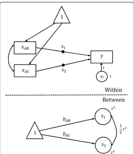
Figures 1 and 2 show the path diagrams for Eqs. (6) and (7) with fixed and random effects, respectively, dem-onstrating how to use the multilevel SEM to undertake the random effect network meta-analysis for example

data. In the level-1 model (the Within-level in Fig. 2),y

is the transformed log odds ratio, and xAB and xAC are

the transformed tAB and tAC, respectively. The filled

cir-cle on the arrow fromxABto yrepresents random slope

that is referred to as s1 in the level-2 model (the

Between-level in Fig. 2). The filled circle on the arrow from xAC to y represents random slope that is referred

to ass2in the level-2 model. The variance ofs1 ands2

is τ2 in Eq. (7), and their covariance is constrained to be1₂τ2. Note that in Fig. 2 there is no random intercept, and the intercept ofyis fixed at 0. The arrows from the variable in triangle tos1ands2indicate that the means of s1and s2are estimated, which give rise toβABand βACin

Eq. (7). The variance of the residual error termeyis fixed at unity. Results show that the log odds ratio for treatment A and B is−0.585 (95% CI: -1.087 to−0.082) and for A and C is−0.711 (95% CI: -1.438 to 0.016).

UWLS for SEM network meta-analysis for example data

To estimate UWLS model with common variance ad-justment factorsϕ1=ϕ2in Eq. (10), we only need to

re-move the constraint on the variance of ey in the fixed effect network meta-analysis model shown in Fig. 1. Table 1 showed results from Mplus for the fixed effect, random effect, and the two UWLS models. Results from Mplus show that ϕ is 3.563, and the log odds ratio for treatment A and B is−0.485 (95% CI: -0.922 to−0.049) and for A and C is−0.600 (95% CI: -1.227 to 0.027). The

Fig. 1Path diagram for the fixed effect network meta-analysis model

point estimates are identical to those in the fixed effect model but the confidence intervals are greater. To esti-mate the UWLS model with unique variance adjustment factors in Eq. (10), we need to create two residual error terms for y: one for studies reporting treatment con-trasts A-B and the other for those reporting treatment contrast A-C. Figure 3 shows the path diagram, wherey

is the transformed log odds ratios and is regressed on

xAB and xAC, which are the transformed variables tAB

and tAC, respectively. Variables gAB and gAC are dummy

variables for studies reporting treatment contrasts A-B and A-C, respectively. The filled circle on the arrow fromgABtoyrepresents random slope that is labelled as s1, and the filled circle on the arrow fromgACtoy

repre-sents random slope that is labelled as s2. The means of s1ands2are fixed at zero, and the variances ofs1ands2

areϕ1andϕ2in Eq. 8, respectively, with their covariance

being fixed at zero. In this model, the residual error for

y is split into two independent random variables s1and s2, and their variances are estimated separately. Results

from Mplus show that the log odds ratio for treatment A and B is−0.484 (95% CI: -0.958 to−0.010) and for A and C is −0.600 (95% CI: -1.075 to −0.125). The point estimates are almost identical to those given by the fixed

effect model, but the confidence intervals are greater. Compared to the confidence intervals reported by the UWLS model with common ϕ, the confidence interval for xABis greater but that forxAC is smaller. This is

be-cause the variance adjustment factors ϕ1 and ϕ2 are

4.288 and 2.031, respectively, indicating a greater degree of heterogeneity within A-B head-to-head trials. This is consistent with results from the traditional pairwise meta-analyses in which the degree of heterogeneity in studies reporting treatment contrast A-B is greater than that of studies reporting contrast A-C.

Discussion

In this article, we demonstrate how to undertake net-work meta-analysis within the statistical framenet-work of structural equation modeling. While issues such as the evaluation of inconsistency between direct and indirect evidence are important and can be integrated into SEM framework, it is beyond the scope of the present study to discuss these issues. Standard statistical software packages for generalized linear mixed modeling may be used to analyze the fixed and random effect models dis-cussed in this article, but SEM software packages are more flexible in specifying complex covariance structure and imposing constraints on parameter estimation. Our results are very close to those reported in previous pub-lications using the command mvmeta for the statistical software package Stata [25, 52]. The estimated random effect variance τ2is 0.877, which is slightly smaller than that given by mvmeta in Stata. Mplus only implements maximum likelihood estimation rather than restricted maximum likelihood estimation [53], but maximum like-lihood estimation tends to under-estimate the variance component in multilevel models [43]. However, metaSEM package in R has implemented restricted maximum likeli-hood estimation and can be used to fit multivariate meta-analysis and network meta-meta-analysis [43, 53].

It is quite straightforward to implement UWLS ap-proach to network meta-analysis with heteroscedastic er-rors in SEM. In the UWLS approach, the between and within-study heterogeneities are considered multiplicative Table 1Results of four SEM models for the example data

Fixed effect model Random effect model UWLS model with commonϕ UWLS model with uniqueϕ

Fixed effect coefficients

bAB −0.485 (−0.717 to−0.254) −0.585 (−1.087 to−0.082) −0.485 (−0.922 to−0.049) −0.485 (−0.958 to−0.010)

bAC −0.600 (−0.932 to−0.268) −0.711 (−1.438 to 0.016) −0.600 (−1.227 to 0.027) −0.600 (−1.075 to−0.125)

Random effect coefficients

τ2

0.877 ϕ

AB 3.563 4.288

AC 3.563 2.031

(ϕσ2

), and this is different from the traditional random ef-fect model, where they are considered additive (σ2

+τ2). The additive random effect assumes that the between and within-study heterogeneities are independent, while the multiplicative random effect assumes that the between and study heterogeneities are related. As within-study heterogeneityσ2is a known quantity, it can then be viewed as the weight for the between-study heterogeneity ϕ. Two recent studies compare the performance of addi-tive or multiplicaaddi-tive heterogeneity in traditional pairwise meta-analyses and found that results of these two models tend to agree but multiplicative model produces narrower confidence intervals [48, 49]. Further research is warranted to compare their performance in network meta-analyses.

Conclusion

SEM provides a useful framework for univariate and multivariate meta-analysis, and its potential as a powerful tool for advanced meta-analysis is still to be explored.

Additional file

Additional file 1:The dataset and Mplus scripts used for statistical analysis. (DOCX 110 kb)

Abbreviations

SEM:Structural equation modeling; UWLS: Unrestricted weighted least squares

Acknowledgements

We would like to thank the editor and three reviewers for their constructive suggestions and comments, which greatly improve our paper.

Availability of data and materials

All data generated or analysed during this study are included in the Additional file 1.

Funding

This project was partly funded by a grant from the Ministry of Science & Technology in Taiwan (grant number: MOST 103–2314 - B - 002 - 032 - MY3).

Authors’contributions

YKT conceived the ideas, obtained the data, undertook the analysis and wrote the draft of the manuscript. YCW helped with the statistical analysis, interpretation of results and the revisions of the manuscript. YKT takes the full responsibility for the integrity of this manuscript. All authors read and approved the final manuscript.

Ethics approval and consent to participate Not applicable.

Consent for publication Not applicable.

Competing interests

The authors declare that they have no competing interests.

Publisher’s Note

Springer Nature remains neutral with regard to jurisdictional claims in published maps and institutional affiliations.

Received: 7 March 2017 Accepted: 10 July 2017

References

1. Sutton AJ, Higgins JPT. Recent developments in meta-analysis. Stat Med. 2008;27(5):625_–50.

2. Caldwell DM, Ades AE, Higgins JPT. Simultaneous comparison of multiple treatments: combining direct and indirect evidence. BMJ. 2005;331(7521): 897–900.

3. Li T, Puhan M, Vedula S, Singh S, Dickersin K. Group TAHNM-aMMW: network meta-analysis-highly attractive but more methodological research is needed. BMC Med. 2011;9(1):79.

4. Tu Y-K. Faggion CM: a primer on network meta-analysis for dental research. ISRN Dent. 2012;2012:10.

5. Cipriani A, Higgins JPT, Geddes JR, Salanti G. Conceptual and technical challenges in network meta-analysis. Ann Intern Med. 2013;159(2):130–7. 6. Dias S, Welton NJ, Sutton AJ, Ades AE. Evidence synthesis for decision

making 1: introduction. Med Decis Mak. 2013;33(5):597_–606.

7. Lumley T. Network meta-analysis for indirect treatment comparisons. Stat Med. 2002;21(16):2313–24.

8. Lu G, Welton NJ, Higgins JPT, White IR, Ades AE. Linear inference for mixed treatment comparison meta-analysis: a two-stage approach. Res Synth Methods. 2011;2(1):43–60.

9. Dias S, Sutton AJ, Ades AE, Welton NJ. Evidence synthesis for decision making 2: a generalized linear modeling framework for Pairwise and network meta-analysis of randomized controlled trials. Med Decis Mak. 2013;33(5):607_–17. 10. Jansen JP, Fleurence R, Devine B, Itzler R, Barrett A, Hawkins N, Lee K,

Boersma C, Annemans L, Cappelleri JC. Interpreting indirect treatment comparisons and network meta-analysis for health-care decision making: report of the ISPOR task force on indirect treatment comparisons good research practices: part 1. Value Health. 2011;14(4):417–28.

11. Lu G, Ades AE. Combination of direct and indirect evidence in mixed treatment comparisons. Stat Med. 2004;23(20):3105–24.

12. Jones B, Roger J, Lane PW, Lawton A, Fletcher C, Cappelleri JC, Tate H. Moneuse P, on behalf of psi health technology special interest group ESs-t: statistical approaches for conducting network meta-analysis in drug development. Pharm Stat. 2011;10(6):523–31.

13. Song F, Altman DG, Glenny A-M, Deeks JJ. Validity of indirect comparison for estimating efficacy of competing interventions: empirical evidence from published meta-analyses. BMJ: Br Med J. 2003;326(7387):472.

14. Song F, Loke YK, Walsh T, Glenny A-M, Eastwood AJ, Altman DG. Methodological problems in the use of indirect comparisons for evaluating healthcare interventions: survey of published systematic reviews. Br Med J. 2009;338(7700):b1147.

15. Glenny A-M, Altman D, Song F, Sakarovitch C, Deeks J, D'amico R, Bradburn M, Eastwood A. Indirect comparisons of competing interventions. Health Technol Assess. 2005;9(26):1–148.

16. Bucher HC, Guyatt GH, Griffith LE, Walter SD. The results of direct and indirect treatment comparisons in meta-analysis of randomized controlled trials. J Clin Epidemiol. 1997;50(6):683_–91.

17. Hasselblad V. Meta-analysis of multitreatment studies. Med Decis Mak. 1998;18(1):37–43.

18. Donegan S, Williamson P, D'Alessandro U, Tudur Smith C. Assessing key assumptions of network meta-analysis: a review of methods. Res Synth Methods. 2013;4(4):291–323.

19. Senn S, Gavini F, Magrez D, Scheen A. Issues in performing a network meta-analysis. Stat Methods Med Res. 2013;22(2):169–89.

20. Hong H, Carlin BP, Shamliyan TA, Wyman JF, Ramakrishnan R, Sainfort F, Kane RL. Comparing Bayesian and Frequentist approaches for multiple outcome mixed treatment comparisons. Med Decis Mak. 2013;33(5):702–14. 21. Lu G, Ades AE. Assessing evidence inconsistency in mixed treatment

comparisons. J Am Stat Assoc. 2006;101(474):447_–59.

22. Higgins JPT, Jackson D, Barrett JK, Lu G, Ades AE, White IR. Consistency and inconsistency in network meta-analysis: concepts and models for multi-arm studies. Res Synth Methods. 2012;3(2):98–110.

23. Salanti G. Indirect and mixed-treatment comparison, network, or multiple-treatments meta-analysis: many names, many benefits, many concerns for the next generation evidence synthesis tool. Res Synth Methods. 2012;3(2):80–97. 24. White IR, Barrett JK, Jackson D, Higgins JPT. Consistency and inconsistency

25. Tu Y-K. Use of generalized linear mixed models for network meta-analysis. Med Decis Mak. 2014;34(7):911_–8.

26. Lu G, Ades AE. Modeling between-trial variance structure in mixed treatment comparisons. Biostatistics. 2009;10(4):792–805.

27. Franchini AJ, Dias S, Ades AE, Jansen JP, Welton NJ. Accounting for correlation in network meta-analysis with multi-arm trials. Res Synth Methods. 2012;3(2):142_–60. 28. Cheung M. Modeling dependent effect sizes with three-level meta-analyses: a structural equation modeling approach. Psychol Methods. 2014;19(2):211–29. 29. Cheung MW. A model for integrating fixed-, random-, and

mixed-effects meta-analyses into structural equation modeling. Psychol Methods. 2008;13(3):182–202.

30. Cheung MWL. Multivariate meta-analysis as structural equation models. Struct Equ Model Multidiscip J. 2013;20(3):429–54.

31. Tu Y-K. Linear mixed model approach to network meta-analysis for continuous outcomes in periodontal research. J Clin Periodontol. 2015;42(2):204–12.

32. Tu YK. Using generalized linear mixed models to evaluate inconsistency within a network meta-analysis. Value Health. 2015;18(8):1120_–5. 33. Tu Y-K. Node-splitting generalized linear mixed models for evaluation of

inconsistency in network meta-analysis. Value Health. 2016;19(8):957–63. 34. Piepho HP, Williams ER, Madden LV. The use of two-way linear mixed

models in multitreatment meta-analysis. Biometrics. 2012;68(4):1269_–77. 35. Hoaglin DC, Hawkins N, Jansen JP, Scott DA, Itzler R, Cappelleri JC, Boersma

C, Thompson D, Larholt KM, Diaz M, et al. Conducting indirect-treatment-comparison and network-meta-analysis studies: report of the ISPOR task force on indirect treatment comparisons good research practices: part 2. Value Health. 2011;14(4):429–37.

36. Salanti G, Higgins JPT, Ades AE, Ioannidis JPA. Evaluation of networks of randomized trials. Stat Methods Med Res. 2008;17(3):279–301.

37. Hong H, Chu HT, Zhang J, Carlin BP. A Bayesian missing data framework for generalized multiple outcome mixed treatment comparisons. Res Synth Methods. 2016;7(1):6–22.

38. Orsini N, Bellocco R, Greenland S. Generalized least squares for trend estimation of summarized dose-response data. Stata J. 2006;6(1):40_–57. 39. Pagliaro L, D'Amico G, Sörensen TIA, Lebrec D, Burroughs AK, Morabito A,

Tiné F, Politi F, Traina M. Prevention of first bleeding in CirrhosisA meta-analysis of randomized trials of nonsurgical treatment. Ann Intern Med. 1992;117(1):59_–70.

40. Kline RB. Principles and practice of structural equation modeling. 4th ed. New York: Guilford publications; 2015.

41. Skrondal A, Rabe-Hesketh S. Generalized latent variable modeling: multilevel, longitudinal and structural equation models. London: Chapman & Hall; 2004. 42. Cheung M, Chan W. Meta-analytic structural equation modeling: a

two-stage approach. Psychol Methods. 2005;10(1):40–64.

43. Cheung MW-L: metaSEM: An R Package for Meta-Analysis using Structural Equation Modeling. Front Psychol 2015, 5.

44. Cheung MWL. Fixed-effects meta-analyses as multiple-group structural equation models. Struct Equ Model Multidiscip J. 2010;17(3):481–509. 45. Cheung MW-L: Meta-analysis: a structural equation modeling approach.

Chichester, UK: John Wiley & Sons; 2015.

46. Greco T, Edefonti V, Biondi-Zoccai G, Decarli A, Gasparini M, Zangrillo A, Landoni G. A multilevel approach to network meta-analysis within a frequentist framework. Contemp clinical trials. 2015;42:51–9. 47. Stanley TD, Doucouliagos H. Neither fixed nor random: weighted least

squares meta-analysis. Stat Med. 2015;34(13):2116–27.

48. Stanley TD, Doucouliagos H. Neither fixed nor random: weighted least squares meta-regression. Res Synth Methods. 2017;8(1):19–42. 49. Mawdsley D, Higgins JPT, Sutton AJ, Abrams KR. Accounting for

heterogeneity in meta-analysis using a multiplicative model-an empirical study. Res Synth Methods. 2017;8(1):43–52.

50. Chaimani A, Higgins JPT, Mavridis D, Spyridonos P, Salanti G. Graphical tools for network meta-analysis in STATA. PLoS One. 2013;8(10):e76654. 51. Chaimani A, Vasiliadis HS, Pandis N, Schmid CH, Welton NJ, Salanti G. Effects

of study precision and risk of bias in networks of interventions: a network meta-epidemiological study. Int J Epidemiol. 2013;

52. White IR. Multivariate random-effects meta-analysis. Stata J. 2009;9(1):40_–56. 53. Cheung MW-L. Implementing restricted maximum likelihood estimation in

structural equation models. Struct Equ Model Multidiscip J. 2013;20(1):157–67.

• We accept pre-submission inquiries

• Our selector tool helps you to find the most relevant journal

• We provide round the clock customer support

• Convenient online submission

• Thorough peer review

• Inclusion in PubMed and all major indexing services

• Maximum visibility for your research

Submit your manuscript at www.biomedcentral.com/submit