Statistical Inference on Random Dot Product Graphs: a
Survey
Avanti Athreya [email protected]
Donniell E. Fishkind [email protected]
Minh Tang [email protected]
Carey E. Priebe [email protected]
Department of Applied Mathematics and Statistics Johns Hopkins University
Baltimore, MD, 2128, USA
Youngser Park [email protected]
Center for Imaging Science Johns Hopkins University Baltimore, MD, 21218, USA
Joshua T. Vogelstein [email protected]
Department of Biomedical Engineering Johns Hopkins University
Baltimore, MD, 21218, USA
Keith Levin [email protected]
Department of Statistics University of Michigan Ann Arbor, MI, 48109, USA
Vince Lyzinski [email protected]
Department of Mathematics and Statistics University of Massachusetts
Amherst, MA, 01003-9305, USA
Yichen Qin [email protected]
Department of Operations, Business Analytics, and Information Systems, College of Business University of Cincinnati
Cincinnati, OH, 45221-0211, USA
Daniel L Sussman [email protected]
Department of Mathematics and Statistics Boston University
Boston, MA, 02215, USA
Editor:Edoardo M. Airoldi
Abstract
The random dot product graph (RDPG) is an independent-edge random graph that is ana-lytically tractable and, simultaneously, either encompasses or can successfully approximate
a wide range of random graphs, from relatively simple stochastic block models to complex latent position graphs. In this survey paper, we describe a comprehensive paradigm for statistical inference on random dot product graphs, a paradigm centered on spectral em-beddings of adjacency and Laplacian matrices. We examine the graph-inferential analogues of several canonical tenets of classical Euclidean inference. In particular, we summarize a body of existing results on the consistency and asymptotic normality of the adjacency and Laplacian spectral embeddings, and the role these spectral embeddings can play in the construction of single- and multi-sample hypothesis tests for graph data. We investigate several real-world applications, including community detection and classification in large social networks and the determination of functional and biologically relevant network prop-erties from an exploratory data analysis of theDrosophilaconnectome. We outline requisite background and current open problems in spectral graph inference.
Keywords: Random dot product graph, adjacency spectral embedding, Laplacian spec-tral embedding, multi-sample graph hypothesis testing, semiparametric modeling
1. Introduction
Random graph inference is an active, interdisciplinary area of current research, bridging combinatorics, probability, statistical theory, and machine learning, as well as a wide spec-trum of application domains from neuroscience to sociology. Statistical inference on ran-dom graphs and networks, in particular, has witnessed extraordinary growth over the last decade: see, for example, Goldenberg et al. (2010) and Kolaczyk (2009) for a discussion of the considerable applications in recent network science of several canonical random graph models.
Of course, combinatorial graph theory itself is centuries old—indeed, in his resolution to the problem of the bridges of K¨onigsberg, Leonard Euler first formalized graphs as mathematical objects consisting of vertices and edges. The notion of a random graph, however, and the modern theory of inference on such graphs, is comparatively new, and owes much to the pioneering work of Erd˝os, R´enyi, and others in the late 1950s. E.N. Gilbert’s short 1959 paper (Gilbert, 1959) considered a random graph for which the existence of edges between vertices are independent Bernoulli random variables with common probability p; roughly concurrently, Erd˝os and R´enyi provided the first detailed analysis of the probabilities of the emergence of certain types of subgraphs within such graphs (Erd˝os and R´enyi, 1960), and today, graphs in which the edges arise independently and with common probability p are known as Erd˝os-R´enyi (or ER) graphs.
networks, we considerlatent positionrandom graphs (Hoff et al., 2002). In a latent position graph, to each vertexiin the graph there is associated an elementxi of the so-calledlatent spaceX, and the probability of connection pij between any two edges iand j is given by a
link or kernel functionκ ∶ X × X → [0,1]. That is, the edges are generated independently
(so the graph is anindependent-edge graph) andpij =κ(xi, xj).
The random dot product graph (RDPG) of Young and Scheinerman (Young and Schein-erman, 2007) is an especially tractable latent position graph; here, the latent space is an appropriately constrained subspace of Euclidean space Rd, and the link function is sim-ply the dot or inner product of the pair of d-dimensional latent positions. Thus, in a
d-dimensional random dot product graph withnvertices, the latent positions associated to the vertices can be represented by an n×dmatrix X whose rows are the latent positions,
and the matrix of connection probabilities P= (Pij)is given byP=XX⊺. Conditional on
this matrix P, the RDPG has an adjacency matrix A= (Aij) whose entries are Bernoulli
random variables with probabilityPij. For simplicity, we will typically consider symmetric, hollowRDPG graphs; that is, undirected, unweighted graphs in whichAii=0, so there are
no self-edges. In our real data analysis of a neural connectome in Section 6.3, however, we describe how to adapt our results to weighted and directed graphs.
In any latent position graph, the latent positions associated to graph vertices can themselves be random; for instance, the latent positions may be independent, identically distributed random variables with some distribution F on Rd. The well-known stochastic blockmodel (SBM), in which each vertex belongs to one ofK subsets known asblocks, with connection probabilities determined solely by block membership (Holland et al., 1983), can be repre-sented as a random dot product graph in which all the vertices in a given block have the same latent positions (or, in the case of random latent positions, an RDPG for which the distribution F is supported on a finite set). Despite their structural simplicity, stochastic block models are the building blocks for all independent-edge random graphs; in Wolfe and Olhede (2013), the authors demonstrate that any independent-edge random graph can be well-approximated by a stochastic block model with a sufficiently large number of blocks. Since stochastic block models can themselves be viewed as random dot product graphs, we see that suitably high-dimensional random dot product graphs can provide accurate ap-proximations of latent position graphs (Tang et al., 2013), and, in turn, independent-edge graphs. Thus, the architectural simplicity of the random dot product graph makes it par-ticularly amenable to analysis, and its near-universality in graph approximation renders it expansively applicable. In addition, the cornerstone of our analysis of random dot product graphs is a set of classical probabilistic and linear algebraic techniques that are useful in much broader settings, such as random matrix theory. As such, the random dot product graph is both a rich and interesting object of study in its own right and a natural point of departure for wider graph inference.
is to construct methods and estimators of graph parameters or graph distributions; and, for these estimators, to analyze their (1) consistency; (2) asymptotic distributions; (3) asymptotic relative efficiency; (4) robustness to model misspecification; and (5) implications for subsequent inference including one- and multi-sample hypothesis testing. In this paper, we summarize and synthesize a considerable body of work on spectral methods for inference in random dot product graphs, all of which not only advance fundamental tenets of this paradigm, but do so within a unified and parsimonious framework. The random graph estimators and test statistics we discuss all exploit theadjacency spectral embedding (ASE) or theLaplacian spectral embedding(LSE), which are eigendecompositions of the adjacency matrix A and normalized Laplacian matrix L = D−1/2AD−1/2, where D is the diagonal
degree matrixDii= ∑j≠iAij.
The ambition and scope of our approach to graph inference means that mere upper bounds on discrepancies between parameters and their estimates will not suffice. Such bounds are legion. In our proofs of consistency, we improve several bounds of this type, and in some cases improve them so drastically that concentration inequalities and asymptotic limit distributions emerge in their wake. We stress that aside from specific cases (see F¨uredi and Koml´os, 1981; Tao and Vu, 2012; Lei, 2016), limiting distributions for eigenvalues and eigenvectors of random graphs are notably elusive. For the adjacency and Laplacian spectral embedding, we discuss not only consistency, but also asymptotic normality, robustness, and the use of the adjacency spectral embedding in the nascent field of multi-graph hypothesis testing. We illustrate how our techniques can be meaningfully applied to thorny and very sizable real data, improving on previously state-of-the-art methods for inference tasks such as community detection and classification in networks. What is more, as we now show, spectral graph embeddings are relevant to many complex and seemingly disparate aspects of graph inference.
comparison of Chernoff information, a long-standing open question of the relative merits of the adjacency and Laplacian graph representations.
Morever, graph embedding plays a central role in the foundational work on hypothesis testing of Tang et al. (2017a) and Tang et al. (2017b) for two-sample graph comparison: these papers provide theoretically justified, valid and consistent hypothesis tests for the semiparamatric problem of determining whether two random dot product graphs have the same latent positions and the nonparametric problem of determining whether two random dot product graphs have the same underlying distributions. This, then, yields a system-atic framework for determining statistical similarity across graphs, which in turn underpins yet another provably consistent algorithm for the decomposition of random graphs with a hierarchical structure Lyzinski et al. (2017). In Levin et al. (2017), distributional re-sults are given for an omnibus embedding of multiple random dot product graphs on the same vertex set, and this embedding performs well both for latent position estimation and for multi-sample graph testing. For the critical inference task of vertex nomination, in which the inference goal is to produce an ordering of vertices of interest (see, for instance Coppersmith, 2014), we find in Fishkind et al. (2015a) an array of principled vertex nom-ination algorithms —-the canonical, maximum likelihood and spectral vertex nomnom-ination schemes—and a demonstration of the algorithms’ effectiveness on both synthetic and real data. In Lyzinski et al. (2016b) the consistency of the maximum likelihood vertex nomina-tion scheme is established, a scalable restricted version of the algorithm is introduced, and the algorithms are adapted to incorporate general vertex features.
Overall, we stress that these principled techniques for random dot product graphs exploit the Euclidean nature of graph embeddings but are general enough to yield meaningful results for a wide variety of random graphs. Because our focus is, in part, on spectral methods, and because the adjacency matrixA of an independent-edge graph can be regarded as a noisy version of the matrix of probabilitiesP(Oliveira, 2009), we rely on several classical results on matrix perturbations, most prominently the Davis-Kahan Theorem (see Bhatia (1997) for the theorem itself, Rohe et al. (2011) for an illustration of its role in graph inference, and Yu et al. (2015) for a very useful variant). We also depend on the aforementioned spectral bounds in Oliveira (2009) and a more recent sharpening due to Lu and Peng (Lu and Peng, 2013). We leverage probabilistic concentration inequalities, such as those of Hoeffding and Bernstein (Tropp, 2015). Finally, several of our results do require suitable eigengaps forP and lower bounds on graph density, as measured by the maximum degree and the size of the smallest eigenvalue ofP. It is important to point out that in our analysis, we assume that the embedding dimensiondof our graphs is known and fixed. In real data applications, such an embedding dimension is not known, and in Section 6.3, we discuss approaches (see Chatterjee, 2015; Zhu and Ghodsi, 2006) to estimating the embedding dimension. Robustness of our procedures to errors in embedding dimension is a problem of current investigation.
average degree, in which differences between vertices in different blocks are assumed to be at the boundary of detectability. Our efforts have a somewhat different flavor, in that we seek to understand the precise behavior of a widely applicable procedure in a more general model. Additionally, we treat sparsity as a secondary concern, and typically do not broach the question of the exact limits of our procedures. Our spectral methods may not be optimal for all random graph models, of course (Krzakala et al., 2013; Kawamoto and Kabashima, 2015), but they are very useful, in that they rely on well-optimized computational methods, can be implemented quickly in many standard languages, extend readily to other models, and serve as a foundation for more complex analyses.
Finally, we would be remiss not to point out that while spectral decompositions and cluster-ings of the adjacency matrix are appropriate for graph inference, they are also of considerable import in combinatorial graph theory: readers may recall, for instance, the combinatorial ratio-cutproblem, whose objective is to partition the vertex set of a graph into two disjoint sets in a way that minimizes the number of edges between vertices in the two sets. The min-imizer of a relaxation to the ratio-cut problem (Fiedler, 1973) is the eigenvector associated to the second smallest eigenvalue of the graph Laplacian L. While we do not pursue more specific combinatorial applications of spectral methods here, we note that Chung (1997) provides a comprehensive overview, and von Luxburg (2007) gives an accessible tutorial on spectral methods.
We organize the paper as follows. In Section 2, we define random dot product graphs and the adjacency spectral embedding, and we recall important linear algebraic background. In Section 4, we discuss consistency, asymptotic normality, and hypothesis testing, as well as inference for hierarchical models. In Section 6, we discuss applications of these results to real data. Finally, in Section 7 we discuss current theoretical and computational difficulties and open questions, including issues of optimal embedding dimension, model limitations, robustness to errorful observations, and joint graph inference. Finally, in A, we provide further details in the proofs of our main results.
2. Definitions, notation, and background
2.1 Preliminaries and notation
We begin by establishing notation. For a positive integern, we let [n] = {1,2,⋯, n}. For a
vectorv∈Rn, we let ∥v∥ denote the Euclidean norm of v. We denote the identity matrix,
zero matrix, and the square matrix of all ones by, I, 0, and J, respectively. We use ⊗ to
denote the Kronecker product. For ann1×n2 matrixH, we let Hij denote itsi, jth entry;
we denote by H⋅j the column vector formed by the j-th column of H; and we denote by
Hi⋅ the row vector formed by the i-th row of H. For a slight abuse of notation, we also let Hi ∈Rn2 denote the column vector formed by transposing the i-th row of H. That is, Hi= (Hi⋅)⊺. Given any suitably specified ordering on eigenvalues of a square matrixH, we
letλi(H)denote thei-th eigenvalue (under such an ordering) ofHandσi(H) = √
λi(H⊺H)
thei-th singular value of H. We let∥H∥ denote the spectral norm of Hand ∥H∥F denote
the rows ofH, so that∥H∥2→∞=maxi∥Hi∥. We denote the trace of a matrix Hby tr(H).
For ann×nsymmetric matrixHwhose entries are all non-negative, we will frequently have
to account for terms related to matrix sparsity, and we defineδ(H) and γ(H) as follows:
δ(H) =max 1≤i≤n
n
∑
j=1
Hij γ(H) = σd
(H) −σd+1(H)
δ(H) (1)
(We remark that whenH is a matrix of connection probabilities for a random graph, δcan be interpreted as the maximum expected degree, andγ relates this quantity to an eigengap that is especially useful in the case of probability matrices of suitably low rank.) In a number of cases, we need to consider a sequence of matrices. We will denote such a sequence by Hn, where nis typically used to denote the index of the sequence. The distinction between a particular elementHnin a sequence of matrices and a particular row Hi of a matrix will be clear from context, and our convention is typically to use n to denote the index of a sequence and ior h to denote a particular row of a matrix. In the case where we need to consider theith row of a matrix that is itself thenth element of a sequence, we will use the notation(Hn)i.
We define agraphGto be an ordered pair of(V, E)whereV is the so-calledvertexornode
set, andE, the set ofedges, is a subset of the Cartesian product ofV×V. In a graph whose
vertex set has cardinality n, we will usually represent V as V = {1,2,⋯, n}, and we say
there is an edge betweeni and j if(i, j) ∈E. Theadjacency matrixA provides a compact
representation of such a graph:
Aij =1 if(i, j) ∈E, andAij =0 otherwise.
Where there is no danger of confusion, we will often refer to a graph Gand its adjacency matrixA interchangeably.
Our focus is random graphs, and thus we will let Ω denote our sample space, F the σ
-algebra of subsets of Ω and P our probability measure P∶ F → [0,1]. We will denote the
expectation of a (potentially multi-dimensional) random variable X with respect to this measure by E. Given an event F ∈ F, we denote its complement by Fc, and we let Pr(F)
denote the probability ofF. As we will see, in many cases we can choose Ω to be subset of Euclidean space. Because we are interested in large-graph inference, we will frequently need to demonstrate that probabilities of certain events decay at specified rates. This motivates the following definition.
Definition 1 (Convergence a.a.s. and w.h.p.) Given a sequence of events {Fn} ∈ F,
where n=1,2,⋯, we say thatFn occursasymptotically almost surely(a.a.s.) ifPr(Fn) →1
asn→ ∞. We say thatFnoccurs with high probability(w.h.p.), and writeFn w.h.p. , if for
anyc0>1, there exists finite positive constantC0 depending onc0 such thatPr[Fnc] ≤C0n−c0
for all n. We note that Fn occurring w.h.p. is stronger than Fn occurring asymptotically almost surely. Morever, Fn occurring with high probability implies, by the Borel-Cantelli Lemma Chung (2001), that with probability 1 there exists an n0 such that Fn holds for all n≥n0.
Definition 2 (Asymptotic notation) If w(n) is a quantity depending on n, we will say
that w is of order α(n) and use the notation w(n) ∼ Θ(α(n)) to denote that there exist
positive constants c, C such that forn sufficiently large,
cα(n) ≤w(n) ≤Cα(n).
When the quantity w(n) is clear andw(n) ∼Θ(α(n)), we sometimes simply write “w is of
order α(n)”. We writew(n) ∼O(n) if there exists a constantC such that fornsufficiently
large, w(n) ≤ Cn. We write w(n) ∼ o(n) if w(n)/n→ 0 as n → ∞, and w(n) ∼ o(1) if
w(n) →0 as n→ ∞. We write w(n) ∼Ω(n) if there exists a constant C such that for all n
sufficiently large, w(n) ≥Cn.
Throughout, we will use C>0 to denote a constant, not depending onn, which may vary
from one line to another.
2.2 Models
Since our focus is ond-dimensional random dot product graphs, we first define anan inner product distributionas a probability distribution over a suitable subset ofRd, as follows:
Definition 3 ( d-dimensional inner product distribution) LetF be a probability dis-tribution whose support is given by suppF = Xd⊂ Rd. We say that F is a d-dimensional
inner product distribution onRd if for all x,y∈ Xd=suppF, we have x⊺y∈ [0,1].
Next, we define a random dot product graph as an independent-edge random graph for which the edge probabilities are given by the dot products of the latent positions associated to the vertices. We restrict our attention here to graphs that are undirected and in which no vertex has an edge to itself.
Definition 4 (RDPG with distribution F) Let F be a d-dimensional inner product distribution with X1,X2, . . . ,Xn
i.i.d.
∼ F, collected in the rows of the matrix
X= [X1,X2, . . . ,Xn]⊺∈Rn×d.
Suppose A is a random adjacency matrix given by Pr[A∣X] = ∏
i<j
(X⊺iXj)Aij(1−X⊺iXj)1−Aij (2)
We then write (A,X) ∼RDPG(F, n) and say that A is the adjacency matrix of a random
dot product graph (RDPG) of dimension or rank at most dand with latent positionsgiven by the rows ofX. IfXX⊺ is, in fact, a rank dmatrix, we say A is the adjacency matrix of a rank d random dot product graph.
Next, for such random dot product graphs, we frequently need to consider thed×dsecond
moment matrix∆, defined as follows:
Definition 5 (Second moment matrix) Suppose A is an adjacency matrix from the random dot product graph model with distribution F. Let X1∼F be one of the i.i.d vectors
of latent positions. Define the second moment matrix ∆ via the expectation
While our notation for a random dot product graph with distribution F is (A,X) ∼
RDPG(F), we emphasize that in this paper the latent positions X are always assumed
to be unobserved. An almost identical definition holds for random dot product graphs with fixed but unobserved latent positions:
Definition 6 (RDPG with fixed latent positions) In the definition 4 given above, the latent positions are themselves random. If, instead, the latent positions are given by a fixed matrix X and, given this matrix, the graph is generated according to Eq.(2), we say that A is a realization of a random dot product graph with latent positions X, and we write A∼RDPG(X).
Remark 7 (Nonidentifiability) Given a graph distributed as an RDPG, the natural task is to recover the latent positions X that gave rise to the observed graph. However, the RDPG model has an inherent nonidentifiability: letX∈Rn×dbe a matrix of latent positions
and let W ∈ Rd×d be a unitary matrix. Since XX⊺ = (XW)(XW)⊺, it is clear that the
latent positions Xand XW give rise to the same distribution over graphs in Equation (2). Note that most latent position models, as defined below, also suffer from similar types of non-identifiability as edge-probabilities may be invariant to various transformations.
As we mentioned, the random dot product graph is a specific instance of the more general latent position random graph with link or kernel function κ. Indeed, the latent positions themselves need not belong to Euclidean space per se, and the link function need not be an inner product.
Definition 8 (Latent position random graph with kernel κ) Let X be a set and κ∶ X × X → [0,1] a symmetric function. Suppose to each i∈ [n] there is associated a point Xi∈ X. Given X= {X1,⋯,Xn} consider the graph with adjacency matrix A defined by
Pr[A∣X] = ∏
i<j
κ(Xi,Xj)Aij(1−κ(Xi,Xj))1−Aij (3)
Then A is the adjacency matrix of a latent position random graph with latent position X and link function κ.
Similarly, we can define independent edge graphs for which latent positions need not play a role.
Definition 9 (Independent-edge graphs) For a matrix symmetric matrix P of proba-bilities, we say that A is distributed as an independent edge graph with probabilities P if
Pr[A∣X] = ∏
i<j
PAij
ij (1−Pij)
1−Aij (4)
By their very structure, latent position random graphs, for fixed latent positions, are independent-edge random graphs. In general, for any latent position graph the matrix of edge probabilities P is given by Pij = κ(Xi,Xj) Of course, in the case of an random
dot product graph with latent position matrixX, the probabilityPij of observing an edge between vertex i and vertexj is simply X⊺iXj. Thus, for an RDPG with latent positions
In order to more carefully relate latent position models and RDPGs, we can consider the set of positive semidefinite latent position graphs. Namely, we will say that a latent position random graph is positive semidefinite if the matrix P is positive semidefinite. In this case, we note that an RDPG can be used to approximate the latent position random graph distribution. (In fact, as we describe further below, new work of Rubin-Delanchy, Tang, and Priebe (Rubin-Delanchy et al., 2017) presents a generalization of the RDPG which allows us to drop the positive semidefiniteness requirement.) The best rank-d approximation of P, in terms of the Frobenius norm (Eckart and Young, 1936), will correspond to a RDPG withd-dimensional latent positions. In this sense, by allowing dto be as large as necessary, any positive semi-definite latent position random graph distribution can be approximated by a RDPG distribution to arbitrary precision (Tang et al., 2013).
While latent position models generalize the random dot product graph, RDPGs can be easily related to the more limitedstochastic blockmodel(SBM) graph (Holland et al., 1983). The stochastic block model is also an independent-edge random graph whose vertex set is partitioned into K groups, called blocks, and the stochastic blockmodel is typically param-eterized by (1) aK×K matrix of probabilities Bof adjacencies between vertices in each of
the blocks, and (2) ablock-assignment vector τ ∶ [n] → [K] which assigns each vertex to its
block. That is, for any two vertices i, j, the probability of their connection is
Pij =Bτ(i),τ(j),
and we typically write A∼SBM(B, τ). Here we present an alternative definition in terms
of the RDPG model.
Definition 10 (Positive semidefinite k-block SBM) We say an RDPG with latent po-sitions X is an SBM with K blocks if the number of distinct rows in X is K, denoted X(1),⋯,X(K) In this case, we define the block membership function τ ∶ [n] ↦ [K] to be a function such that τ(i) =τ(j) if and only if Xi=Xj. We then write
A∼SBM(τ,{X(i)}Ki=1)
In addition, we also consider the case of a stochastic block model in which the block mem-berships of each vertex is randomly assigned. More precisely, letπ∈ (0,1)K with∑nk=1πk=1 and suppose that τ(1), τ(2), . . . , τ(n) are now i.i.d. random variables with distribution
Categorical(π); that is, Pr(τ(i) = k) = πk for all k. Then we say A is an SBM with
i.i.d block memberships, and we write
A∼SBM(π,{X(i)}).
We also consider thedegree-corrected stochastic block model (Karrer and Newman, 2011):
Definition 11 (Degree Corrected SBM) We say an RDPG is a degree-corrected stochas-tic block model (DCSBM) with K blocks if there exist K unit vectors y1, . . . , yK ∈Rd such that for eachi∈ [n], there existsk∈ [K] and ci∈ (0,1) such thatXi=ciyk.
For an important generalization that offers more flexibility in block memberships, we con-sider themixed-membership stochastic block model (MMSBM) of Airoldi et al. (2008):
Definition 13 (Mixed Membership SBM) We say an RDPG is a mixed membership stochastic block model (MMSBM) with K blocks if there existsKunit vectorsy1, . . . , yK ∈Rd
such that for each i ∈ [n], there exists α1, . . . , αK > 0 such that ∑Kk=1αk = 1 and Xi = ∑Kk=1αkyk.
Remark 14 The mixed membership SBM allows for each vertex to be in a mixture of different blocks. Additionally, note that every RDPG is a MMSBM for some choice of K.
Our next theorem summarizes the relationship between these models.
Theorem 15 Considered as statistical models for graphs—to wit, sets of probability dis-tributions on graphs—the positive-semidefinite K-block SBM is a subset of the K-block DCSBM and theK-block MMSBM. Both the positive semidefiniteK-block DCSBM andK -block MMSBM are subsets of the RDPG model withK-dimensional latent positions. Finally, the union of all possible RDPG models, without restriction of latent position dimension, is dense in the set of positive semidefinite latent position models.
We emphasize that, as mentioned previously, very recent work of Rubin-Delanchy, Priebe, and Tang (Rubin-Delanchy et al., 2017) on the generalized random dot product graph (gRDPG) extends the essential construction of the random dot product graph to encom-pass non-positive-semidefinite stochastic block models and mixed membership block models, and the gRDPG possesses an elegant uniqueness property that permits the representation of mixed membership as a convex combination of extreme points in a simplex. So, while we impose some restrictions on positive-definiteness here, these are primarily for ease of exposition. Our methodology is general enough to encompass networks that exhibit both homophily and heterophily (see, for example, Hoff, 2007). Moreoever, when considering normalized latent positions for random dot product graphs, our requirement of positive definiteness is, in effect, a degree-corrected “affinity.” Also, as we show in Section 6.3, our techniques have proven empirically appropriate in the analysis of certain directed graphs, wherein we consider right- and left-singular vectors in a singular value decomposition of the adjacency matrix.
2.3 Embeddings
Since we rely on spectral decompositions, we begin with describing the notations for the spectral decomposition of the rank dpositive semidefinite matrix P=XX⊺.
Definition 16 (Spectral Decomp. of P) Since P is symmetric and positive semidefi-nite, let P=UPSPUP⊺ denote its spectral decomposition, with UP∈Rn×d having
orthonor-mal columns and SP∈Rd×d a diagonal matrix with nonincreasing entries (SP)1,1≥ (SP)2,2≥ ⋯ ≥ (SP)d,d>0.
Definition 17 (Adjacency spectral embedding (ASE)) Given a positive integer d≥
1, the adjacency spectral embedding (ASE) of A into Rd is given by Xˆ =UAS1A/2 where
∣A∣ = [UA∣U⊥A][SA⊕S⊥A][UA∣U⊥A]⊺
is the spectral decomposition of ∣A∣ = (ATA)1/2 and SA is the diagonal matrix of the d
largest eigenvalues of∣A∣ andUA is then×dmatrix whose columns are the corresponding
eigenvectors.
The intuition behind the notion of adjacency spectral embedding is as follows. Our goal is to estimate the latent position matrixX. Now, if the matrixPwere actually observable, then the spectral embedding of P, given by UPS1P/2, is simply some orthogonal transformation
of X. Of course, Pis typically not observable; instead we observeA, a noisy version of P. The ASE will be a good estimate ofX provided that the noise does not greatly impact the embedding—that is, ifAandPare suitably close. As we will see shortly, one can show that
∥A−XX⊺∥ =O(∥X∥) =o(∥XX⊺∥)with high probability (Oliveira, 2009; Lu and Peng, 2013;
Tropp, 2015; Lei and Rinaldo, 2015). That is to say, A can be viewed as a comparatively small perturbation of XX⊺. Weyl’s inequality or the Kato-Temple inequality (Cape et al., 2017a; Kato, 1950) guarantee that the eigenvalues of A are “close” to the eigenvalues of XX⊺. In addition, by the Davis-Kahan theorem (Davis and Kahan, 1970), the subspace spanned by the top d eigenvectors of XX⊺ is well-approximated by the subspace spanned by the topdeigenvectors ofA.
Having defined the adjacency spectral embedding, we next define the analogous Laplacian spectral embedding, which uses the spectral decomposition of the normalized Laplacian matrix.
Definition 18 (Laplacian Spectral Embedding (LSE)) LetL(A) =D−1/2AD−1/2
de-note the normalized Laplacian ofA where D is the diagonal matrix whose diagonal entries Dii= ∑j/=iAij. Given a positive integerd≥1, the Laplacian spectral embedding (LSE) of A into Rd is given byX˘ =UL(A)S˜1A/2 where
∣L(A)∣ = [UL(A)∣U⊥L(A)][SL(A)⊕S⊥L(A)][UL(A)∣U⊥L(A)]
⊺
is the spectral decomposition of∣L(A)∣ = (L(A)⊺L(A))1/2 andSL(A)is the diagonal matrix
containg the dlargest eigenvalues of ∣L(A)∣ on the diagonal andUL(A) is the n×dmatrix
whose columns are the corresponding eigenvectors.
3. Core proof techniques: probabilistic and linear algebraic bounds
In this section, we give an overview of the core background results used in our proofs. While we defer to the appendix the proofs of our primary results on consistency and normality for spectral graph estimates, we provide key background here to allow the reader a consolidated, accessible guide to the essential linear algebraic foundations of our approach. The key tools to several of our results on consistency and normality of the adjacency spectral embedding depend on a triumvirate of matrix concentration inequalities, the Davis-Kahan Theorem, and detailed bounds via the power method.
3.1 Concentration inequalities
Concentration inequalities for real- and matrix-valued data are a critical component to our proofs of consistency for spectral estimates. We make use of classical inequalities, such as Hoeffding’s inequality, for real-valued random variables, and we also exploit more recent work on the concentration of sums of random matrices and matrix martingales around their expectation. For a careful study of several important matrix concentration inequalities, see Tropp (2015).
We begin by recalling Hoeffding’s inequality, which bounds the deviations between a sample mean of independent random variables and the expected value of that sample mean.
Theorem 19 Let Xi, 1≤i≤n, be independent, bounded random variables defined on some
probability space (Ω,F,P). Suppose ai, bi are real numbers such that ai≤Xi≤bi. Let X¯ be
their sample mean:
¯
X= 1
n n
∑
i=1
Xi
Then
Pr(X¯−E(X¯) ≥t) ≤exp(
[−2n2t2] ∑ni=1(bi−ai)2
) (5)
and
Pr(∣X¯ −E(X¯)∣ ≥t) ≤2 exp(
[−2n2t2] ∑ni=1(bi−ai)2
) (6)
For an undirected, hollow RDPG with probability matrixP,E(Aij) =Pij for all i≠j. As
such, one can regard A as a “noisy” version of P. It is tempting to believe that A and P are close in terms of the Frobenius norm, but this is sadly not true; indeed, it is easy to see that
∥A−P∥2F =Θ(∥P∥2F)
To overcome this using only Hoeffding’s inequality, we can instead consider the difference
(A2−P2)ij, which is a sum of independent random variables. Hence, Hoeffding’s inequality
implies that
∣(A2−P2)ij∣2=o(∣P2ij∣2)
somewhat stronger and more elegant results can be shown by considering the spectral norm instead. In particular, a nontrivial body of recent work on matrix concentration implies that, under certain assumptions on the sparsity of P, the spectral norm of A−P can be
well-controlled. We focus on the following important results of Oliveira (2009) and Tropp (2015) and further improvements of Lu and Peng (2013) and Lei and Rinaldo (2015), all of which establish that the A andP are close in spectral norm.
Theorem 20 (Spectral norm control of A−P) Suppose Let A be the adjacency
ma-trix of an independent-edge random graph on [n] with matrix of edge probabilities P. For
any constant c, there exists another constant C, independent of n and P, such that if
δ(P) >Clnn, then for any n−c<η<1/2,
Pr(∥A−P∥ ≤4 √
δ(P)ln(n/η)) ≥1−η. (7)
In Lu and Peng (2013), the authors give an improvement under slightly stronger density assumptions1:
Theorem 21 (Refined spectral norm control of A−P) With notation as above,
sup-pose there exist positive constants such that for nsufficiently large,δ(P) > (logn)4+a. Then
for anyc>0 there exists a constant C depending on c such that
P(∥A−P∥ ≤2 √
δ(P) +Cδ1/4(P)lnn) ≥1−n−c. (8)
3.2 Matrix perturbations and spectral decompositions
The above results formalize our intuition that A provides a “reasonable” estimate for P. Moreover, in the RDPG case, wherePis of low rank and is necessarily positive semidefinite, these results have implications about the nonnegativity of the eigenvalues ofA. Specifically, we use Weyl’s Theorem to infer bounds on the differences between the eigenvalues of A and P from the spectral norm of their difference, and the Gerschgorin Disks Theorem to infer lower bounds on the maximum row sums ofPfrom assumptions on the eigengap ofP (since bothPandAare nonnegative matrices, one could also obtain the same lower bounds by invoking the Perron-Frobenius Theorem). For completeness, we recall the Gerschgorin Disks Theorem and Weyl’s Theorem (these can be found, for example, in Horn and Johnson, 1985). The former relates the eigenvalues of a matrix to the sums of the absolute values of the entries in each row, and the latter establishes bounds on the differences in eigenvalues between a matrix and a perturbation.
Theorem 22 (Gerschgorin Disks) Let H be a complex n×nmatrix, with entries Hij.
For i∈ {1,⋯, n}let Ri = ∑j≠i∣Hij∣. Let the ith Gerschgorin disk D(Hii, Ri) be the closed
disk centered at Hii with radius Ri. Then every eigenvalue of Hlies within at least one of the Gershgorin discs D(Hii, Ri).
1. A similar bound is provided in Lei and Rinaldo (2015), but withδ(P)defined asδ(P) =nmaxijPijand
Theorem 23 (Weyl) Let M,H, and R be n×n Hermitian matrices, and suppose M = H+R. Suppose H and R have eigenvalues ν1 ≥ ⋯ ≥ νn and r1 ≥ ⋯ ≥ rn, respectively.
Suppose the eigenvalues ofM are given by µ1≥ ⋯ ≥µn. Then νi+rn≤µi≤νi+r1
From our random graph model assumptions and our graph density assumptions, we can conclude that with for sufficiently largen, the topdeigenvalues ofA will be nonnegative: Remark 24 (Nonnegativity of the top d eigenvalues of A) SupposeA∼RDPG(X).
Since P = XX⊺, it is necessarily positive semidefinite, and thus has nonnegative
eigen-values. If we now assume that γ(P) > c0 for some constant c0, then along with the
Gershgorin Disks Theorem, guarantee that the top d eigenvalues of P are all of order
δ(P), and our rank assumption on P mandates that the remaining eigenvalues be zero.
If δ(P) >log4+a
′
n, the spectral norm bound in (8) applies, ensuring that for n sufficiently large, ∥A−P∥2 ∼O(
√
δ(P)) with high probability. Thus, by Weyl’s inequality, we see that
the top deigenvalues ofA are, with high probability, of orderδ, and the remaining are, with high probability, within √δ of zero.
Since P = XX⊺ = UPS1P/2(UPS1P/2)⊺ and A is close to P, it is intuitively appealing to
conjecture that, in fact, ˆX=UAS1/2
A should be close to some rotation of UPS
1/2
P . That is,
ifX is the matrix of true latent positions—-so XW=UPS1P/2 for some orthogonal matrix W—then it is plausible that ∥Xˆ −XW∥F ought to be comparatively small. To make this
precise, however, we need to understand how both eigenvalues and eigenvectors of a matrix behave when the matrix is perturbed. Weyl’s inequality addresses the former. The impact of matrix perturbations on associated eigenspaces is significantly more complicated, and the Davis-Kahan Theorem (Davis and Kahan, 1970; Bhatia, 1997) provides one approach to the latter. The Davis-Kahan has a significant role in several approaches to spectral estimation for graphs: for example, Rohe, Chatterjee, and Yu leverage it in Rohe et al. (2011) to prove the accuracy of spectral estimates (specifically, the graph Laplacian) in high-dimensional stochastic blockmodels. The version we give below is from Yu et al. (2015), which is a user-friendly guide to the the Davis-Kahan Theorem and its statistical implications.
The Davis-Kahan Theorem is often stated as a result on canonical angles between subspaces. To that end, we recall that ifU and V are two n×d matrices with orthonormal columns,
then we define the vector ofdcanonicalorprincipal angles between their column spaces to be the vector Θ such that
Θ= (θ1=cos−1σ1,⋯, θd=cos−1σd)⊺
whereσ1,⋯, σd are the singular values ofU⊺V. We define the matrix sin(Θ)to be thed×d
diagonal matrix for which sin(θ)ii=sinθi.
Theorem 25 (A variant of Davis-Kahan) Suppose Hand H′ are two symmetric n×n
matrices with real entries with spectrum given by λ1≥λ2⋯ ≥λn and λ′1≥λ′2⋯ ≥λ′n,
Let 0 < d ≤ n be fixed, and let V be the matrix of whose columns are the eigenvectors
v1,⋯, vd, and similarly V′ the matrix whose columns are the eigenvectors v′1,⋯v′n. Then
∥sin(Θ)∥F ≤ 2 √
d∥V−V′∥
λd(H) −λd+1(H)
.
Observe that if we assume that P is of rank d and has a sufficient eigengap, the Davis-Kahan Theorem gives us an immediate bound on the spectral norm of the difference between UAU⊺A and UPU⊺P in terms of this eigengap and the spectral norm difference of A−P,
namely:
∥UAU⊺A−UPU⊺P∥ =max
i ∥sin(θi)∥ ≤
C∥A−P∥
λd(P) .
Recall that the Frobenius norm of a matrix Hsatisfies
(∥H∥F)2= ∑
i,j
H2ij =tr(H⊺H) ≥ ∥H∥2
and further that ifH is of rankd, then
(∥H∥F)2≤d∥H∥2
and hence for rankdmatrices, spectral norm bounds are easily translated into bounds on the Frobenius norm. It is worth noting that Rohe et al. (2011) guarantees that a difference in projections can be transformed into a difference between eigenvectors themselves: namely, given the above bound for∥UAU⊺A−UPU⊺P∥F, there is a constantC and an orthonormal
matrixW ∈Rd×d such that
∥UPW−UA∥F ≤C √
d∥A−P∥ λd(P)
. (9)
While these important results provide the backbone for much of our theory, the detailed bounds and distributional results described in the next section rely on a decomposition of ˆX in terms of (A−P)UPS−1/2
P and a remainder. This first term can be viewed as an
application of the power method for finding eigenvectors. Additionally, standard univariate and multivariate concentration inequalities and distributional results can be readily applied to this term. On the other hand, the remainder term can be shown to be of smaller order than the first, and much of the technical challenges of this work rely on carefully bounding the remainder term.
4. Spectral embeddings and estimation for RDPGs
of the adjacency matrix of an ER graph. Again, despite their model simplicity, Erd˝ os-R´enyi graphs veritably teem with open questions; to cite but one example, in a very recent manuscript, Arias-Castro and Verzhelen (Arias-Castro and Verzelen, 2014) address, in the framework of hypothesis testing, the question of subgraph detection within an ER graph.
Moving up to the slightly more heterogeneous stochastic block model, we again find a rich literature on consistent block estimation in stochastic block models. Fortunato (Fortunato, 2010) provides an overview of partitioning techniques for graphs in general, and consistent partitioning of stochastic block models for two blocks was accomplished by Snijders and Nowicki (Snijders and K.Nowicki, 1997) and for equal-sized blocks by Condon and Karp in 2001. For the more general case, Bickel and Chen (Bickel and Chen, 2009) demonstrate a stronger version of consistency via maximizing Newman-Girvan modularity (Newman, 2006) and other modularities. For a growing number of blocks, Choi et al. (Bickel et al., 2013) prove consistency of likelihood based methods, and Bickel et al. (Bickel et al., 2011) provide a method to consistently estimate the stochastic block model parameters using sub-graph counts and degree distributions. This work and the work of Bickel and Chen (Bickel and Chen, 2009) both consider the case of very sparse graphs. In Airoldi et al. (2008), Airoldi et al. define the important generalization of a mixed-membership stochastic block-model, in which block membership may change depending on vertex-to-vertex interactions, and the authors demonstrate methods of inference for the mixed membership and block probabilities.
Rohe, Chatterjee and Yu show in Rohe et al. (2011) that spectral embeddings of the Lapla-cian give consistent estimates of block memberships in a stochastic block model, and they also demonstrate how to deploy spectral approaches to estimate block memberships even in strongly heterophilic block models. One of the earliest corresponding results on the consistency of the adjacency spectral embedding the estimation of block memberships is given by Sussman and coauthors in Sussman et al. (2012), where it is proved that for a stochastic block model with K blocks and a rank dblock probability matrix B, clustering the rows of the adjacency spectral embedding via k-means clustering (see Pollard, 1981) results in at most logn vertices being misclassified. An improvement to this can be found in Fishkind et al. (2013), where consistency recovery is possible even if the rank of the embedding dimension is unknown.
In Lyzinski et al. (2014), under the assumption of distinct eigenvalues for the second moment matrix ∆ (recall we defined this in 5) of a random dot product graph, it is shown that clustering the rows of the adjacency spectral embedding results in asymptotically almost surely perfect recovery of the block memberships in a stochastic blockmodel—that is, for sufficiently largen, the probability of all vertices being correctly assigned is close to 1. An especially strong recovery is exhibited here: it is shown that in the 2 → ∞ norm, ˆX is
sufficiently close to a rotation of the the true latent positions. In fact, each row in ˆX is withinClogn/
√
nof the corresponding row inX. Unlike a Frobenius norm bound, in which it is possible that some rows of ˆX may be close to the true positions but others may be significantly farther away, this 2→ ∞bound implies that the adjacency spectral embedding
Furthermore, in Tang et al. (2017a), one finds a nontrivial tightening of the Frobenius norm bound for the difference between the (rotated) true and estimated latent positions: in fact the Frobenius norm is not merely bounded from above by a term of order logn, but rather concentrates around a constant. This constant-order Frobenius bound forms the basis of a principled two-sample hypothesis test for determining whether two random dot product graphs have the same generating latent positions (see Section 5.2).
In Lyzinski et al. (2017), the 2 → ∞-norm bound is extended even to the case when the
second moment matrix ∆ does not have distinct eigenvalues. This turns out to be criti-cal in guaranteeing that the adjacency spectral embedding can be effectively deployed for community detection in hierarchical block models. We present this bound for the 2 → ∞
norm in some detail here; it illustrates the confluence of our key techniques and provides an effective roadmap for several subsequent results on asymptotic normality and two-sample testing.
4.1 Consistency of latent position estimates
We state here one of our lynchpin results on consistency, in the 2→ ∞norm, of the adjacency
spectral embedding for latent position estimation of a random dot product graph. We given an outline of the proof here, and refer the reader to the Appendix A for the details, which essentially follow the proof given in Lyzinski et al. (2017). We emphasize our setting is a sequence of random dot product graphs An ∼RDPG(Xn) for increasing n and thus we
make the following density assumption on Pn asnincreases:
Assumption 1 LetAn∼RDPG(Xn)forn≥1be a sequence of random dot product graphs withAn being a n×n adjacency matrix. Suppose thatXn is of rankdfor all nsufficiently
large. Suppose also that there exists constantsa>0andc0>0such that for all nsufficiently
large,
δ(Pn) =max
i n
∑
j=1
(Pn)ij ≥log4+a(n); γ(Pn) = λd (Pn)
δ(Pn) ≥c0.
We remark that this assumption is, in essence, a restriction on graph sparsity, and not a particular onerous one; d-dimensional random dot product graphs with i.i.d latent po-sitions that are not “too” degenerate will meet these requirements, and bounds on δ of the polylogarithmic order given above are quite common (see Oliveira, 2009; Lu and Peng, 2013).
Our consistency result for the 2 → ∞ norm is Theorem 26 below. In the proof of this
fluidly between the two versions of a random dot product graph, adapting our results as appropriate in each case.
In the Appendix, we give a detailed proof of Theorem 26 and we point out the argument used therein also sets the stage for the central limit theorem for the rows of the adjacency spectral embedding given in Subsection 4.2.
Theorem 26 Let An∼RDPG(Xn) for n≥1 be a sequence of random dot product graphs
where the Xn is assumed to be of rank d for all n sufficiently large. Denote by Xˆn the adjacency spectral embedding ofAnand let (Xˆn)i and(Xn)i be thei-th row ofXˆnandXn,
respectively. Let En be the event that there exists an orthogonal transformation Wn∈Rd×d
such that
max i ∥(
ˆ
Xn)i−Wn(Xn)i∥ ≤ Cd
1/2log2n
δ1/2(P
n)
where C>0is some fixed constant andPn=XnX⊺n. ThenEnoccurs asymptotically almost
surely; that is, Pr(En) →1 as n→ ∞.
Under the stochastic blockmodel, previous bounds on ∥X−Xˆ∥F implied that k-means
applied to the rows of ˆX would approximately correctly partition the vertices into their the true blocks with up to O(logn) errors. However, this Frobenius norm bound does not
preclude the possibility of large outliers in the individual rows ofX−Xˆ. The improvements
provided by Theorem 26 overcome this hurdle and, as shown in Lyzinski et al. (2014), under suitable sparsity and eigengap assumptions, k-means applied to ˆX will exactly correctly partition the vertices into their true blocks. This implication demonstrates the importance of improving the overall bounds and in focusing on the correct metrics for a given task—in this case, for instance, block identification.
While we defer the proof of this result to the Appendix, in A.1, we provide a brief outline and note several key ingredients here. First is a lemma guaranteeing the existence of an orthogonal matrixW∗ such that
∥W∗SA−SPW∗∥F =O((logn)δ1/2(P)
That is, there is an approximate commutativity between right and left multiplication of the corresponding matrices of eigenvalues by this orthogonal transformation. The second essential component is, at heart, a bound inspired by the power method. Specifically, we show that there exists an orthogonal matrix
∥Xˆ −XW∥ = ∥(A−P)UPSP−1/2∥F +O((logn)δ−1/2)
Finally, from this point, establishing the bound on the 2 → ∞ norm is a consequence of
Hoeffding’s inequality applied to sums of the form
∑
k
(Aik−PikUkj)
.
The 2→ ∞ bound in Theorem 26 has several important implications. As we mentioned,
restrictive assumptions on the the second moment matrix, and illustrate how this can be used to cluster vertices in an SBM perfectly; that is, with no vertices misclassified. In addition, in Lyzinski et al. (2014), we show that clustering the rows of the ASE can be useful for inference in a degree-corrected stochastic block model as well. In Section 6, we see that because of Theorem 26, the adjacency spectral embedding and a novel angle-based clustering procedure can be used for accurately identifying subcommunities in an affinity-structured, hierarchical stochastic blockmodel (Lyzinski et al., 2017). In the next section, we see how our proof technique here can be used to obtain distributional results for the rows of the adjacency spectral embedding.
4.2 Distributional results for the ASE
In the classical statistical task of parametric estimation, one observes a collection of i.i.d observationsX1,⋯, Xnfrom some family of distributionsFθ∶θ∈Θ, where Θ is some subset
of Euclidean space, and one seeks to find a consistent estimatorT(X1,⋯, Xn) forθ. As we
mentioned in Section 1, often a next task is to determine the asymptotic distribution, as
n→ ∞, of a suitable normalization of this estimatorT. Such distributional results, in turn,
can be useful for generating confidence intervals and testing hypotheses.
We adopt a similar framework for random graph inference. In the previous section, we demonstrate the consistency of the adjacency spectral embedding for the true latent position of a random dot product graph. In this section, we establish the asymptotic normality of the rows of this embedding and the Laplacian spectral embedding. In the subsequent section, we examine how our methodology can be deployed for multisample graph hypothesis testing.
We emphasize that distributional results for spectral decompositions of random graphs are comparatively few. The classic results of F¨uredi and Koml´os (F¨uredi and Koml´os, 1981) describe the eigenvalues of the Erd˝os-R´enyi random graph and the work of Tao and Vu (Tao and Vu, 2012) is focused on distributions of eigenvectors of more general random matrices under moment restrictions, but Athreya et al. (2016) and Tang and Priebe (2018) are among the only references for central limit theorems for spectral decompositions of adjacency and Laplacian matrices for a wider class of independent-edge random graphs than merely the Erd˝os-R´enyi model. Apart from their inherent interest, these limit theorems point us to current open questions on efficient estimation and the relative merits of different estimators and embeddings, in part by rendering possible a comparison of asymptotic variances and allowing us to quantify relative efficiency (see Tang et al. (2016) and to precisely conjecture a decomposition of the sources of variance in different spectral embeddings for multiple graphs (see Levin et al., 2017).
Specifically, we show that for a d-dimensional random dot product graph with i.i.d latent positions, there exists a sequence of d×d orthogonal matrices Wn such that for any row
indexi,√n(Wn(Xˆn)i− (Xn)i)converges as n→ ∞to a mixture of multivariate normals. Theorem 27 (Central Limit Theorem for rows of ASE) Let (An,Xn) ∼RDPG(F)
the cdf of a (multivariate) Gaussian with mean zero and covariance matrix Σ, evaluated at x∈Rd. Then there exists a sequence of orthogonal d-by-d matrices (Wn)∞n=1 such that for
allz∈Rd and for any fixed index i,
lim n→∞Pr[n
1/2
(XˆnWn−Xn)
i≤z] = ∫suppFΦ(z,Σ(x))dF(x), where
Σ(x) =∆−1E[(x⊺X1− (x⊺X1)2)X1X⊺1]∆−1; and∆=E[X1X⊺1]. (10)
We also note the following important corollary of Theorem 27 for whenF is a mixture ofK
point masses; that is,(X,A) ∼RDPG(F)is a K-block stochastic blockmodel graph. Then
for any fixed index i, the event thatXi is assigned to block k∈ {1,2, . . . , K} has non-zero probability and hence one can condition on the block assignment of Xi to show that the conditional distribution of√n(Wn(Xˆn)i− (Xn)i)converges to a multivariate normal. This
is in contrast to the unconditional distribution being a mixture of multivariate normals as given in Theorem 27.
Corollary 28 (SBM) Assume the setting and notations of Theorem 27 and let
F =
K
∑
k=1
πkδνk, π1,⋯, πK >0,∑
k πk=1
be a mixture of K point masses in Rd where δνk is the Dirac delta measure at νk. Then
there exists a sequence of orthogonal matrices Wn such that for allz∈Rdand for any fixed
index i,
P{ √
n(WnXˆn−Xn)i ≤z∣Xi=νk} Ð→Φ(z,Σk) (11)
where Σk=Σ(νk) is as defined in Eq. (52).
We relegate the full details of the proof of this central limit theorem to the Appendix, in Section A.2, but a few points bear noting here. First, both Theorem 27 and Corollary 28 are very similar to results proved in Athreya et al. (2016), but with the crucial difference being that we no longer require that the second moment matrix ∆= E[X1X⊺1] of X1 ∼ F have
We stress that this central limit theorem depends on a delicate bounding of a sequence of so-called residual terms, but its essence is straightforward. Specifically, there exists an orthogonal transformationW∗ such that we can write the ith row of the matrix
√
n(UAS1/2
A −UPS
1/2
P W∗)
as
√
n(UAS1A/2−UPS1P/2W∗)i= √
n(A−P)UPSP−1/2W∗)i+Residual terms (12)
where the residual terms are all of order O(n−1/2logn) in probability. Now, to handle the
first term in Eq.(12), we can condition on a fixed latent position Xi = xi, and when this
is fixed, the classical Lindeberg-Feller Central Limit Theorem establishes the asymptotic normality of this term. The order of the residual terms then guarantees, by Slutsky’s Theorem, the desired asymptotic normality of the gap between estimated and true latent positions, and finally we need only integrate over the possible latent positions to obtain a mixture of normals.
4.3 An example under the stochastic block model
To illustrate Theorem 27, we refer the reader to Athreya et al. (2016), from which we reproduce the following simulation. Consider random graphs generated according to a stochastic block model with parameters
B = [0.42 0.42
0.42 0.5] and π= (0.6,0.4). (13)
In this model, each node is either in block 1 (with probability 0.6) or block 2 (with prob-ability 0.4). Adjacency probabilities are determined by the entries in B based on the block memberships of the incident vertices. The above stochastic blockmodel corresponds to a random dot product graph model in R2 where the distribution F of the latent posi-tions is a mixture of point masses located at x1 ≈ (0.63,−0.14) (with probability 0.6) and
x2≈ (0.69,0.13) (with probability 0.4).
We sample an adjacency matrixAfor graphs onnvertices from the above model for various choices ofn. For each graphG, let ˆX∈Rn×2 denote the embedding ofA and let ˆXi⋅ denote
theith row of ˆX. In Figure 1, we plot thenrows of ˆXfor the various choices ofn. The points are denoted by symbols according to the block membership of the corresponding vertex in the stochastic blockmodel. The ellipses show the 95% level curves for the distribution of ˆXi for each block as specified by the limiting distribution.
We estimate the covariance matrices for the residuals. The theoretical covariance matrices are given in the last column of Table 1, where Σ1 and Σ2are the covariance matrices for the residual√n(Xˆi−Xi) when Xi is from the first block and second block, respectively. The
−0.3 0.0 0.3
0.55 0.60 0.65 0.70 0.75
x
y
block
1
2
(a)n=1000
−0.25 0.00 0.25
0.60 0.65 0.70 0.75
x
y
block
1
2
(b)n=2000
−0.2 0.0 0.2 0.4
0.60 0.65 0.70
x
y
block
1
2
(c)n=4000
−0.3 −0.2 −0.1 0.0 0.1 0.2
0.600 0.625 0.650 0.675 0.700 0.725
x
y
block
1
2
(d)n=8000
Figure 1: Plot of the estimated latent positions in a two-block stochastic blockmodel graph on n vertices. The points are denoted by symbols according to the block membership of the corresponding vertices. Dashed ellipses give the 95% level curves for the distributions as specified in Theorem 27. Figure duplicated from Athreya et al. (2016).
n 2000 4000 8000 16000 ∞
ˆ
Σ1 [.58 .54
.54 16.56] [
.58 .63 .63 14.87] [
.60 .61 .61 14.20] [
.59 .58 .58 13.96] [
.59 .55 .55 13.07]
ˆ
Σ2 [.58 .75
.75 16.28] [
.59 .71 .71 15.79] [
.58 .54 .54 14.23] [
.61 .69 .69 13.92] [
.60 .59 .59 13.26]
Table 1: The sample covariance matrices for √n(Xˆi−Xi) for each block in a stochastic
blockmodel with two blocks. Here n ∈ {2000,4000,8000,16000}. In the last column are
We also investigate the effects of the multivariate normal distribution as specified in Theo-rem 27 on inference procedures. It is shown in Sussman et al. (2012, 2014) that the approach of embedding a graph into some Euclidean space, followed by inference (for example, clus-tering or classification) in that space can be consistent. However, these consistency results are, in a sense, only first-order results. In particular, they demonstrate only that the error of the inference procedure converges to 0 as the number of vertices in the graph increases. We now illustrate how Theorem 27 may lead to a more refined error analysis.
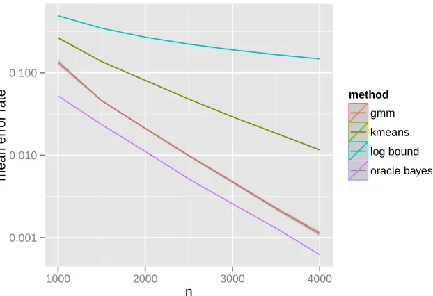
We construct a sequence of random graphs onnvertices, wherenranges from 1000 through 4000 in increments of 250, following the stochastic blockmodel with parameters as given above in Eq. (13). For each graphGnonnvertices, we embedGnand cluster the embedded vertices of Gn via Gaussian mixture model and K-means clustering. Gaussian mixture model-based clustering is done using the MCLUST implementation of (Fraley and Raftery, 1999). We then measure the classification error of the clustering solution. We repeat this procedure 100 times to obtain an estimate of the misclassification rate. The results are plotted in Figure 2. For comparison, we plot the Bayes optimal classification error rate under the assumption that the embedded points do indeed follow a multivariate normal mixture with covariance matrices Σ1 and Σ2 as given in the last column of Table 1. We also plot the misclassification rate of (Clogn)/n as given in Sussman et al. (2012) where
the constant C was chosen to match the misclassification rate of K-means clustering for
n =1000. For the number of vertices considered here, the upper bound for the constant
C from Sussman et al. (2012) will give a vacuous upper bound of the order of 106 for the misclassification rate in this example. Finally, we recall that the 2 → ∞ norm bound
of Theorem 26 implies that, for large enough n, even the k-means algorithm will exactly recover the true block memberships with high probability (Lyzinski et al., 2016a).
For yet another application of the central limit theorem, we refer the reader to Suwan et al. (2016), where the authors discuss the assumption of multivariate normality for estimated latent positions and how this can lead to a significantly improved empirical-Bayes framework for the estimation of block memberships in a stochastic blockmodel.
4.4 Distributional results for Laplacian spectral embedding
We now present the analogous central limit theorem results of Section 4.2 for the normal-ized Laplacian spectral embedding (see Definition 18). We first recall the definition of the Laplacian spectral embedding.
Theorem 29 (Central Limit Theorem for rows of LSE) Let (An,Xn) ∼ RDPG(F)
for n≥1 be a sequence of d-dimensional random dot product graphs distributed according
to some inner product distribution F. Let µ and ∆˜ denote the quantities
µ=E[X1] ∈Rd; ∆˜ =E[X1X
⊺
1 X⊺1µ ] ∈R
d×d
. (14)
Also denote byΣ˜(x) the d×dmatrix
E[(
˜ ∆−1X1
X⊺1µ −
x 2x⊺µ)(
X⊺1∆˜−1 X⊺1µ −
x⊺ 2x⊺µ)
(x⊺X1−x⊺X1X⊺1x)
0.001 0.010 0.100
1000 2000 3000 4000
n
mean error r
ate method
gmm
kmeans
log bound
oracle bayes
Figure 2: Comparison of classification error for Gaussian mixture model (red curve), K-Means (green curve), and Bayes classifier (cyan curve). The classification errors for each
n ∈ {1000,1250,1500, . . . ,4000} were obtained by averaging 100 Monte Carlo iterations
Then there exists a sequence of d×d orthogonal matrices (Wn) such that for each fixed
index iand any x∈Rd,
Pr{n(Wn(X˘n)i−√ (Xn)i
∑j(Xn)⊺i(Xn)j
) ≤x} Ð→ ∫ Φ(x,Σ˜(y))dF(y) (16)
When F is a mixture of point masses—specifically, when A ∼ RDPG(F) is a stochastic
blockmodel graph—we also have, below, the following limiting conditional distribution for
n(Wn(X˘n)i−√ (Xn)i
∑j(Xn)⊺i(Xn)j
).
Theorem 30 Assume the setting and notations of Theorem 29 and let
F =
K
∑
k=1
πkδνk, π1,⋯, πK >0,∑
k πk=1
be a mixture of K point masses in Rd. Then there exists a sequence of d×d orthogonal
matrices Wn such that for any fixed indexi,
P{n(Wn(X˘n)i−√ νk
∑lnlν⊺kνl
) ≤z∣ (Xn)i=νk} Ð→Φ(z,Σ˜k) (17)
where Σ˜k =Σ˜(νk) is as defined in Eq. (15) and nk for k∈ {1,2, . . . , K} denote the number
of vertices inA that are assigned to blockk.
Remark 31 As a special case of Theorem 30, we note that if A is an Erd˝os-R´enyi graph on n vertices with edge probability p2 – which corresponds to a random dot product graph where the latent positions are identically p – then for each fixed index i, the normalized Laplacian embedding satisfies
n(X˘i−√1
n)
d
Ð→ N (0,1−p 2 4p2 ). Recall that X˘i is proportional to 1/
√
di where di is the degree of the i-th vertex. On the other hand, the adjacency spectral embedding satisfies
√
n(Xˆi−p)Ð→ N (d 0,1−p2).
As another example, let A be sampled from a stochastic blockmodel with block probability matrix B = [p
2 pq
pq q2] and block assignment probabilities (π,1−π). Since B has rank 1, this model corresponds to a random dot product graph where the latent positions are either p
with probability π or q with probability 1−π. Then for each fixed index i, the normalized
Laplacian embedding satisfies
n(X˘i−√ p
n1p2+n2pq
)Ð→ N (d 0,πp(1−p
2)+(1−π)q(1−pq)
4(πp+(1−π)q)3 )if Xi=p, (18)
n(X˘i−√ q
n1pq+n2q2
)Ð→ N (d 0,πp(1−pq)+(1−π)q(1−q 2)
where n1 andn2=n−n1 are the number of vertices ofAwith latent positionsp andq. The
adjacency spectral embedding, meanwhile, satisfies
√
n(Xˆi−p)Ð→ N (d 0,πp
4(1−p2)+(1−π)pq3(1−pq)
(πp2+(1−π)q2)2 )if Xi=p, (20)
√
n(Xˆi−q)Ð→ N (d 0,πp
3q(1−pq)+(1−π)q4(1−q2)
(πp2+(1−π)q2)2 )if Xi=q. (21)
We present a sketch of the proof of Theorem 29 in the Appendix, in Section A.3. Due to the intricacy of the proof, however, even in the Appendix we do not provide full details; we instead refer the reader to Tang and Priebe (2018) for the complete proof. Moving forward, we focus on the important implications of these distributional results for subsequent inference, including a mechanism by which to assess the relative desirability of ASE and LSE, whichvary depending on inference task.
5. Implications for subsequent inference
The previous sections are devoted to establishing the consistency and asymptotic normality of the adjacency and Laplacian spectral embeddings for the estimation of latent positions in an RDPG. In this section, we describe several subsequent graph inference tasks, all of which depend on this consistency: specifically, nonparametric clustering, semiparametric and nonparametric two-sample graph hypothesis testing, and multi-sample graph inference.
5.1 Nonparametric clustering: a comparison of ASE and LSE via Chernoff information