PMU Placement Methods in Power Systems based on Evolutionary Algorithms and GPS Receiver

PMU Placement Methods in Power Systems Based on

Evolutionary

Algorithms and GPS Receiver

M. R. Mosavi* and A. Akhyani*

Abstract: In this paper, optimal placement of Phasor Measurement Unit (PMU) using

Global Positioning System (GPS) is discussed. Ant Colony Optimization (ACO), Simulated Annealing (SA), Particle Swarm Optimization (PSO) and Genetic Algorithm (GA) are used for this problem. Pheromone evaporation coefficient and the probability of moving from state x to state y by ants are introduced into the ACO. The modified algorithm overcomes the ACO in obtaining global optimal solution and convergence speed, when applied to optimize the PMU placement problem. We also compare this simulation with SA, PSO and GA to examine the capability of ACO in the search of optimal solution. The fitness function includes observability, redundancy and the number of PMU. Logarithmic Least Square Method (LLSM) is used to calculate the weights of fitness function. The suggested optimization method is applied in 30-bus IEEE system and the simulation results show that modified ACO results are better than PSO and SA, but it has nearly the same results as GA.

Keywords: Evolutionary Algorithms, Global Positioning System, Optimal Placement,

Phasor Measurement Unit.

1 Introduction1

The Global Positioning System (GPS), which is a satellite based system, is the main synchronizing source which is used to provide an accurate time reference on the communication networks, and its broad availability makes it possible to obtain, at each point of the tested system, a clock signal that is synchronized with the one generated in other remote places. Currently, GPS is the only satellite system with sufficient availability and accuracy for the most scattered monitoring and control applications in distribution systems. Synchronizing signals could also be broadcast from a terrestrial location, and with respect to this, radio broadcasts are probably the least expensive [1, 2].

The accurate time reference signal, which the standard refers to for the evaluation of the synchronized phasors, is the Universal Time Coordinated (UTC). For this purpose, GPS receivers specify that the synchronization signal must have a basic repetition rate of one Pulse Per Second (1 PPS). The synchronizing source shall have sufficient availability, reliability, and accuracy to meet power system requirements [3].

Monitoring the operating state of the system and assessing its stability in real time has been recognized as

Iranian Journal of Electrical & Electronic Engineering, 2013. Paper first received 27 Sep. 2012 and in revised form 15 Apr. 2013. * The authors are with the Department of Electrical Engineering, Iran University of Science and Technology, Tehran, Iran.

E-mails: [email protected] and [email protected].

a task of paramount importance and a tool to prevent blackouts. Phasor Measurement Units (PMUs) is used to estimate system stability [4].

Recently, PMUs equipped with GPS is applied in power systems monitoring and state estimation. PMUs can directly measure the voltage amplitudes and phase angles of key buses in power systems with high accuracy. Since GPS provides tiny synchronization errors, the interests are concentrated on where and how many PMUs should be implemented in a power system with the least cost and with the largest degree of observability [5].

Because of the strong correlation between PMUs and the GPS, PMUs began to spread greatly after the great improvement in the satellite techniques and communications [6].

The PMU Placement Optimization (PPO) is to minimize the number of PMUs and maximize the redundancy by optimizing the PMU’s locations, while keeping all the nodes voltage phasors observable. A specially tailored non-dominated sorting Genetic Algorithm (GA) for a PMU placement problem is proposed in [7] as a methodology to find these Pareto-optimal solutions.

Taking the full network observability of power system operation states and the least number of PMUs as an objective function, an improved optimal PMU placement algorithm is proposed in [8]. In this algorithm, GA is effectively combined with the Particle

Swarm Optimization (PSO) algorithm to ensure that the optimal solution can be obtained [8].

In this paper, we want to perform PPO with modified Ant Colony Optimization (ACO), GA, PSO and Simulated Annealing (SA) and these results compared with each other. At first, we introduce observability in power systems. Then we talk about fitness function and evolutionary algorithms and finally simulation results and compression with each other.

2 Power System Observability with PMUs

Power system observability might be described by graph theory [9]. An N-bus power system is represented as a no oriented graph G N, B , where is a set of graph vertices containing all system nodes, and B is a

set of graph edges containing all system branches. PMUs could measure the voltages and all the branch current phasors at the nodes where they are placed. The phasors of the nodes without PMUs, may be prepared via pseudo-measurement. The pseudo-measurement includes three parameters:

1. If the voltages at the both ends of a branch have been known, the current of that branch can be calculated using Ohm’s laws,

2. If a node voltage and one branch current have been known, the voltage of another end of the branch can be calculated using Ohm’s laws, and

3. If a node where all but one branch current are known, the last unknown current can be calculated using Kirchhoff’s law [10].

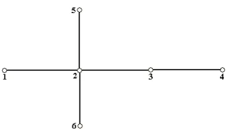
Totally observability is devided to numerical and topological strategies. In this paper, observability is calculated by topological strategy. In topological strategy observability function ( fi ) is calculated for

every node of the network using incidence matrix [11]. For example for the network that is shown in Fig. 1 the incidence matrix is:

⎥ ⎥ ⎥ ⎥ ⎥ ⎥ ⎥ ⎥ ⎦ ⎤ ⎢ ⎢ ⎢ ⎢ ⎢ ⎢ ⎢ ⎢ ⎣ ⎡ = 1 0 0 0 1 0 0 1 0 0 1 0 0 0 1 1 0 0 0 0 1 1 1 0 1 1 0 1 1 1 0 0 0 0 1 1

A ₍₁₎

and the observability function is:

⎪ ⎪ ⎪ ⎪ ⎩ ⎪⎪ ⎪ ⎪ ⎨ ⎧ + = + = + = + + = + + + + = + = = 6 2 6 5 2 5 4 3 4 4 3 2 3 6 5 3 2 1 2 2 1 1 x x f x x f x x f x x x f x x x x x f x x f

F ₍₂₎

Fig. 1 Example for 6-bus system

where ‘+’ is OR (logical operator) and xi is defined:

⎩ ⎨ ⎧ = Otherwise i node at installed is PMU a If xi ; 0 ; 1 (3)

3 Problem Formulation

In this section, at the beginning, we determine fitness function. Then, we talk about ACO, GA, PSO and SA algorithm and values of its parameter in these problems.

3.1 Fitness Function

Fitness function for placement in this paper is defined: 1 * 3 * 2 1 * 1 )

( W J

PMU N W Nb i fi W X

J ∑ + +

=

= (4)

where ∑ = Nb i

fi

1 shows the observability value of the power system, N MU is the number of PMUs in the power system network. If we assume that the favorite level of redundancy is 2, J is the difference between the favorite and the real values. To calculate the weights of fitness function, we consider the importance of each factor in comparison to the other factors. Table 1 is used to calculate the scales of pair-wise comparisons.

Once a hierarchy framework is constructed, users are requested to make a pair-wise comparison matrix at each hierarchy and compare each other by using a scale pair-wise comparison [12]. The below 3*3 matrix is calculated according to Table 1:

⎥ ⎥ ⎥ ⎥ ⎥ ⎥ ⎦ ⎤ ⎢ ⎢ ⎢ ⎢ ⎢ ⎢ ⎣ ⎡ 1 9 1 5 1 9 1 3 5 3 1 1 (5)

Table 1 Scale for pair-wise comparisons [12].

Relative

intensity Definition

1 Equal value

3 Slightly more value

5 Essential or strong value

7 Very strong value

9 Extreme value

2,4,6,8 _{between two adjacent judgments} Intermediate values

W can be calculated as follows:

∏ = _∏ = = n j n j ij a ij a i W 1 1 (6)

where a_ij is an item of this matrix is the number of

fitness function factors. This function is called Logarithmic Least Square Method (LLSM), which is a part of the Analytical Hierarchy Process (AHP) algorithm [12].

3.2 ACO Algorithm

To solve several discrete optimization problems, ACO metaheuristic, a new population-based approach was proposed in [13]. An ant is a simple computational agent in the ACO algorithm. It iteratively constructs solutions for the problem. The intermediate solutions are a kind of solution states. At each repetition of the algorithm, each ant goes from a state x to state y, to make a more complete intermediate solution. Therefore, each ant k create a set AK x of feasible expansions to its current state at each repetition, and moves to one of these in probability. For ant k, the probability p of moving from state toward state depends on the combination of two values. The attractiveness of the move shows how expert it has been in the past to make that particular move. has been calculated by some heuristic method indicating a priori desirability of that move and the trail level τ of the move. The trail level indicates a posteriori indication of the desirability of that move. Trails are updated often when all ants have completed their solutions, decreasing or increasing the level of trails corresponding to moves that were a part of "unsuitable" or "suitable" solutions, respectively. In general, the k ant moves from state x to state y with this probability: ∑ = ) )( ( ) )( ( β η α τ β η α τ xy xy xy xy k xy

p (7)

where τ is the amount of pheromone which is deposited for change from state x to y. α 0 controls the effect of τ , η is the desirability of the state transition xy (previous knowledge, generally, where d is the distance) and β 0 controls the influence of

η . When all the ants have completed a solution, the trails are updated as follows:

k xy k

xy k

xy ρ τ τ

τ =(1− ) +Δ (8) where τ is the amount of pheromone that is deposited for a state transition xy, ρ is the pheromone evaporation coefficient and ∆τ is the amount of pheromone which is deposited, generally given by:

⎪ ⎩ ⎪ ⎨ ⎧ = Δ Otherwise tour its in xy curve uses k ant If k L Q k xy ; 0 ;

τ (9)

in which LK is the cost of the k ant's tour (generally length) and Q is constant [14]. The ant system simply repeats a main loop where ants construct in parallel their solutions, thus updating the trail levels. The function of the algorithm depends on the correct tuning of several parameters. α and β are relative importance of trail and attractiveness, τij 0 is initial trail level, ρ is trail persistence, is the number of ants, and Q is used for explaining to be of high quality solutions with low cost. The algorithm is as follow:

Step1: Initialization

Initialize τij and ηij, (ij).

Step2: Construction

For each ant k (currently in state i) do repeat

choose in probability the state to move into. append the chosen move to the k-th ant's set tabuk. until ant k has completed its solution.

end for

Step3: Trail update

For each ant move (ij) do compute ∆τij.

update the trail matrix. end for

Step4: Terminating condition

If not (end test) go to step 2 [15].

In this problem, we assume 0, 1 in Eq. (8) and Q 1 in Eq. (9).

3.3 Genetic Algorithm

In GA, a population of strings (chromosomes), which encode candidate solutions (individuals) to optimize the result, evolves toward better solutions. Classically, solutions are represented in binary as strings of zeros and ones, but other encodings could also be considered. The evolution often begins from a population of randomly generated individuals and occurs in generations. In each repetition, every individual fitness in the population is estimated, multiple individuals are stochastically chosen from the current population (according to their fitness), and modified (recombined and maybe mutated randomly) thus forming a new population. The new population is then handled in the next repetition of the algorithm. Generally, the algorithm is finished whenever a satisfactory fitness level has been reached for the population or a maximum number of generations has been made. If the algorithm has been finished because of a maximum number of generations, an accepted solution may or may not have been reached [16].

GAs find application in different fields of engineering, artificial intelligence, economics, manufacturing, physics, mathematics, etc. GAs require: 1) a genetic representing of the solution zone, and 2) a fitness function to estimate the solution zone. A standard representing of the solution is an array of bits. Arrays of other kinds and constructions could be used in the same manner. The most important characteristic that makes these genetic representations suitable is that their sections are easily aligned because of their fixed size, which reaches simple crossover operations. Variable length representations could also be considered, but crossover implementation is more complex in this situation. In genetic programming tree-like representations are used and in programming graph-form representations are considered. The fitness function has to be defined in the genetic representation. The fitness function measures the quality of the represented solution. The fitness function always depends on the problem. Sometimes it is hard or even infeasible to define the fitness expression; in such cases, interactive GA should be used. When the genetic representation and the fitness function has been defined, a GA begins to initialize a new population of solutions. GA then tries to improve the population using repetitive application of the mutation, crossover, inversion and selection operators [17].

3.3.1 Initialization

Initially a lot of individual solutions are stochastically generated to form an initial population. The population size depends on the problem characteristic, but may contain several thousands of possible answers. Classically, the population is stochastically generated, allowing the entire range of feasible answers. Sometimes the solutions might be

"seeded" in zones where optimal solutions are possible to be found [17].

3.3.2 Selection

In each generation, a proportion of the population is selected to bring about a new generation. Individual solutions are chosen through a fitness-based process, where generally more suitable solutions are more fortunate to be selected. Definite selection methods assess the fitness of each solution and preferentially choose the best answers. Other methods assess only a random sample of the population, as the latter process is probably very time-consuming [17].

3.3.3 Reproduction

Now is the time to generate a second generation population of answers from those chosen through crossover and mutation. For each new answer to be produced, a pair of "parent" answers should be selected for breeding from the pool chosen in the past. By producing a "child" answer using the previous methods of crossover and mutation, a new answer is made which generally shares many of the features of its "parents". New parents are chosen for each new child, and the process keeps doing until a new population of answers of appropriate size is generated. Despite the fact that reproduction methods which are based on the use of two parents are more "biology inspired", several researches suggest that more than two "parents" generate better quality chromosomes. Ultimately these processes bring about the next generation population of chromosomes which is totally different from the initial one. Usually the average fitness will have been increased by this procedure for the population, since only the best organisms from the first generation are chosen for breeding, along with a small proportion of less fit answers, because of the reasons already said above. Although crossover and mutation are considered as the principal genetic operators, it is feasible to use other operators like regrouping, colonization-extinction, or migration in our GAs [17].

3.3.4 Termination

This generational process should be repeated until a termination condition is reached. Common terminating conditions are: 1) an answer is found that meets the minimum criteria, 2) fixed number of generations are reached, 3) assigned budget reached, 4) the best ranking answer's fitness is meeting or has met a plateau so successive repetitions no longer produce any better results, 5) manual verifying, and 6) combinations of the above. Typical generational GA procedure [17]:

Step1: Select the initial population of individuals.

Step2: Estimate the fitness of each individual in that

population.

Step3: Repeat on this generation until termination

(sufficient fitness achieved, time limit, and etc.): 1. Select the best-fit individuals for reproduction. 2. Breed new individuals through crossover and

mutation operations to give birth to offspring. 3. Evaluate the individual fitness of new

individuals.

4. Replace least-fit population with new individuals.

3.4 Particle Swarm Optimization

PSO is a computational method in artificial intelligence that optimizes a problem by iteratively keeping improving a candidate solution regarding a given measure of quality. Our problem is optimized by PSO. In PSO there is a population of candidate solutions, here named particles, which move around in the search-space based on simple mathematical formulae over the particle's velocity and position. The movement of each particle is influenced by its local best position and is also directed towards the best positions in the search-space, which are updated when better positions are found by other particles. This method is expected to move the swarm towards the best answers. PSO is originally introduced by Eberhart, Kennedy and Shi and was first planned to simulate social behavior, as a representation of the movement of mechanism in a fish school or bird flock. The algorithm became simplified and it was considered to perform optimization. The book by Kennedy and Eberhart explains many philosophical points of view of PSO and swarm intelligence. A great survey of PSO uses is made by Poli [18].

PSO is a metaheuristic because it makes almost no assumptions about the problem being optimized and can search large spaces of candidate solutions. However, metaheuristics like PSO do not guarantee that an optimal solution is found. PSO does not use the gradient of our problem, which means it is not necessary for our optimization problem to be differentiable, although it was required for classical optimization methods like gradient descent and quasi-newton. Therefore PSO can be used in optimization problems that are noisy, partially irregular, change over time, and etc.

Formally, let f: Rn _{→ R be the objective function} that must be minimized. The function takes a candidate answer as argument which is in the form of a vector of real numbers and produces a real number as output which shows the fitness of the given candidate answer. The gradient of f is not determined. The aim is to find an answer: a for which f(a) ≤ f(b) for all b in our search-space, which mean a is the global minimum. Maximization can be done by considering h f instead. Presume that is the number of particles in the swarm, each of them have a position xi Rn in our search-space and a velocity vi R . Presume that p is the best known position of particle i and presume that g

is the best known position of the entire swarm. A basic PSO algorithm would be [19]:

Step1: For each particle i = 1, ..., S perform:

1. Initialize the position of the particle with a uniformly distributed random vector: xi~U(blow, bup), where blow and bup are the lower and upper boundaries of the search-space. 2. Initialize the best known position of the

particle to its initial position: pi← xi.

3. If (f(pi) < f(g)) update the best known position of the swarm: g ← pi.

4. Initialize the velocity of the particle: vi~U(-|bup-blow| , |bup-blow|).

Step2: Until a termination criterion is reached (e.g. the

number of iterations performed), repeat: 5. For each particle i = 1, ..., S perform:

ƒ For each dimension d = 1, ..., n perform:

ƒ Pick random numbers:

rp, rg~U(0,1).

ƒ Update the velocity of the particle: vi,d ←ωvi,d +φprp(pi,d-xi,d) + φgrg(gd-xi,d).

ƒ Update the position of the particle: xi← xi + vi.

ƒ If (f(xi)< f(pi)) perform:

ƒ Update the best known position of the particle: pi← xi.

ƒ If (f(pi)< f(g)) update the best known position of the swarm: g ← pi.

Step3: Now g holds the best found answer.

The parameters ω, φp, and φg are chosen by the practitioner and control the behavior and efficacy of PSO [19].

Kennedy and Eberhart [17] have adapted the PSO to search in binary spaces. For binary discrete search space, by applying a sigmoid transformation to the velocity component Eq. (10) to press the velocities into a range [0,1], and force the component values of the position of particles to be zeros or ones. The equation for updating positions is then replaced by Eq. (11) [20]. sigmod V, _{V ,} (10)

x 1 ; if rand sigmod V,

0 ; otherwise (11) That Vi,d is the velocity of the particles.

3.5 Simulated Annealing

Here SA is a generic probabilistic metaheuristic for the global optimization problem of finding a good estimation to the global optimum of a given function in a really large search space. It is often applied when the search space is discrete. For specific problems, SA

might be more efficient than exhaustive enumeration providing the goal is merely to find a good answer in a fixed amount of time, rather than the best possible answer. SA comes from annealing in metallurgy, a technique which has heating and controlled cooling of a material to increase the size of its crystals and decrease their defects. The heat forces the atoms to be unstuck from their initial positions, that is a local minimum of the internal energy, and go randomly through states of higher energy, the slow cooling gives them more chance to find configurations with lower internal energy than the initial one. Comparing with this physical process, each step of SA tries to replace the current answer by a random answer (selected according to a candidate distribution, usually constructed to sample from answers near the current answer). The new answer might be accepted with a probability which depends both on the difference between the corresponding function values and on a global parameter T (temperature). T is gradually decreased during the algorithm. The dependency is such that the selection between the previous and the current answer is almost random when T is large, but increasingly chooses the better or "downhill" answer (in a minimization problem) as T goes to zero. The allowance for "uphill" moves saves the procedure from becoming stuck at local optima. In SA, each point s of the search-space is similar to a state of some physical system, and also the function E s to be minimized is similar to the internal energy of the system in that state. The aim is to bring the system, from a random initial state, to a state with the minimum possible energy [21]. A basic SA algorithm is as follows. Presume that s is an initial solution and is an initial temperature.

Repeat

S Generate a neighbor of the solution C ∆E Objective s Objective s If (∆E 0), Then

s s

Else If EXP(∆E/T 0~1 , Then s s

End If T T Dt

Until T< Temperature of stop condition [22].

4 Simulation Results

4.1 Case Study

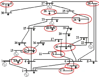
The PMU placement was performed for an active model of the 30-bus IEEE network, using ACO, GA, PSO and SA that its topology is shown in Fig. 2 [23]. We assume that the observability is complete. Therefore only the answers are selected which make all nodes’ voltage phasors observable.

Therefore PMUs are installed at all important locations of the network to be observed [25].

4.2 Discussion

In modified ACO, 30 ants travel on the nodes of network, the tour is finished when the network has been observable. When the tour is completed by 30 ants, pheromone matrix changes, and new ants begin traveling with new values of pheromone. This process continues to find the optimum result. Fig. 3 shows the placement of PMUs in IEEE 30-bus using the proposed ACO.

Fig. 2 Schematic of 30-bus IEEE system [24]

Fig. 4 shows the best of fitness function values in any repeat using the proposed ACO. In this simulation, 10 PMUs are placed in the buses 1, 5, 9, 10, 12, 19, 24, 25, 28 and 29. The result value of fitness function is 8.63.

Table 2 shows that the number of iterations in ACO, appeared in [10], is more than that in modified ACO, therefore we could improve convergence speed compared to [10].

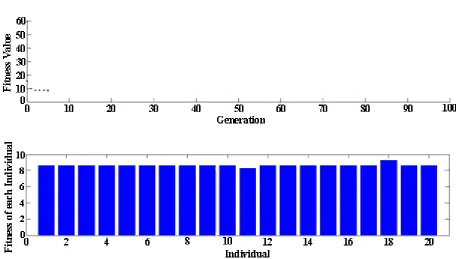
The result of the simulation using GA, is 10 PMUs on IEEE 30-bus. The final value of fitness function is 8.62. Fig. 5 shows the placement of PMUs using the

proposed GA. Fig. 6 shows the fitness function values in any generation and shows individual fitnesses.

Table 2 Comparing the number of iterations (convergence speed).

Methods Number of iterations

Proposed ACO 20

Introduced ACO in [10] 35

Fig. 3 Placement of PMU in IEEE 30-bus using the proposed ACO

Fig. 4 Best of fitness function using the proposed ACO

Fig. 5 Placement PMU using the proposed GA

Fig. 6 The fitness function values the using proposed GA

After the optimized placement on procedure is completed using PSO, it is shown that only 11 PMUs are needed with the complete observability and a good redundancy condition is satisfied. Value of fitness

function is 9.1. Fig. 7 shows the PMU placement using the proposed PSO. Fig. 8 shows the cost function values in any repeat.

Fig. 7 Placement PMU using the proposed PSO

Fig. 8 The cost function values using the proposed PSO

After the placement on network is completed using proposed SA, it is shown that only 11 PMUs are needed with the complete observability and a suitable redundancy condition is satisfied. The value of the fitness function is 9.4. Fig. 9 shows the PMU placement using the proposed SA and Fig. 10 shows fitness function values in any repeat.

Simulation results show that the ACO finds a smaller fitness function value than PSO’s and SA’s, but equals to GA’s. They also show that the numbers of PMUs are less in ACO than that in PSO and SA algorithms, but it is equal to that in GA. Table 3 shows this comparison.

Table 3 Comparison of algorithms in PPO.

Algorithms Numbers of PMU Fitness function value

ACO 10 8.63

GA 10 8.62

PSO 11 9.1

SA 11 9.4

Fig. 9 Placement PMU using the proposed SA

Fig. 10 The fitness function values any repeat using the proposed SA

5 Conclusion

With the development and strategic positioning of PMUs in significant numbers, there is an increasing need for PPO. In this paper a modified ACO method for PPO problems was suggested. ACO was compared to PSO, SA and GA. The proposed methods were applied to the PPO problems in 30-bus IEEE standard power systems to show its effectiveness. The proposed algorithms were validated by simulation. The results obtained are indicative of the fact that the optimal placement of PMU increases the accuracy of the obtained estimates and efficiency of the bad data detection algorithms. Increasing the number of buses in power system shows that ACO, in case of equality

between the number of ants and buses, gets a better result in comparison to the SA’s and PSO’s. However the ACO’s results are equal to the GA’s. Also convergence speed in modified ACO was improved in comparison to the last works. The future works should include the consideration of zero injection bus and changes in the topology of the power systems. The limitations of GPS in the aspect of timing in fitness function should also be considered.

Acknowledgment

The authors would like to thank Iran Distribution Management Company, for their valuable support during the authors’ research work.

References

[1] Mosavi M. R., “GPS Receivers Timing Data Processing using Neural Networks: Optimal Estimation and Errors Modeling”, Journal of Neural Systems, Vol. 17, No. 5, pp. 383-393, 2007.

[2] Chen Y., Reale D., Dickens J., Holt S., Mankowski J. and Kristiansen M., “Phased Array Pulsed Ring-Down Source Synchronization with a GPS Based Timing System”, IEEE Transactions on Dielectrics and Electrical Insulation, Vol. 18, No. 4, pp. 1071-1078, 2011. [3] Refan M. H. and Valizadeh H., “Computer

Network Time Synchronization using a Low Cost GPS Engine”, Iranian Journal of Electrical and Electronic Engineering, Vol. 8, No. 3, pp. 206-216, 2012.

[4] Meliopoulos A. P. S., Cokkinides G. J., Wasynczuk O., Coyle E., Bell M., Hoffmann C., Nita-Rotar C., Downr T., Tsoukalas L. and Gao R., “PMU Data Characterization and Application to Stability Monitoring”, IEEE Conference on Power Systems, pp. 151-158, 2006.

[5] Carta A., Locci N., Muscas C. and Sulis S., “A Flexible GPS-Based System for Synchronized Phasor Measurement in Electric Distribution Networks”, IEEE Transaction on Instrumentation and Measurement, Vol. 57, No. 11, pp. 2450-2456, 2008.

[6] Wentao Z., Yufeng A., Xujun Z. and Ye W., “The Implementation of Synchronized Phasor Measurement and Its Applications in Power System”, Proceedings of the Conference on Electrical Engineering, Vol. 1, pp. 139-143, 1996.

[7] Milosevic B. D. and Begovic M., “Nondominated Sorting Genetic Algorithm for Optimal Phasor Measurement Placement”, IEEE Power Engineering Review, Vol. 22, No. 12, pp. 61-61, 2002.

[8] Gao Y., Hu Z., He X. and Liu D., “Optimal Placement of PMUs in Power Systems based on Improved PSO Algorithm”, IEEE Conference on Industrial Electronics and Applications, pp. 2464-2469, 2008.

[9] Baldwin T. L., Mili L., Boisen M. B. and Adapa R., “Power System Observability with Minimal Phasor Measurement Placement”, IEEE Transactions on Power Systems, Vol. 8, No. 2, pp. 707-715, 1993.

[10] Wang B., Liu D. and Xiong L., “Advance ACO System in Optimizing Power System PMU Placement Problem”, IEEE Conference on Power Electronics and Motion Control, pp. 2451-2453, 2009.

[11] Krumpholz G. R., Clements K. A. and Davis P. W., “Power System Observability: A Practical Algorithm using Network Topology”, IEEE

Transactions on Power Apparatus and System, Vol. PAS-99, No. 4, pp. 1534-1542, 1980. [12] Ariff H., Salit M. S., Ismail N. and Nukman Y.,

“Use of Analytical Hierarchy Process (AHP) for Selecting the Best Design Concept”, Asian Journal of Teknologi, pp. 1-18, 2008.

[13] Abadi M. and Jalili S., “Ant Colony Optimization Algorithm for Network Vulnerability Analysis”, Iranian Journal of Electrical and Electronic Engineering, Vol. 2, Nos. 3 &4, pp. 106-120, 2006.

[14] Colorni A., Dorigo M. and Maniezzo V., “Distributed Optimization by Ant Colonies”, International Conference on Artificial Life, pp. 134-142, 1991.

[15] Caldeira J. L., Azevedo R. C., Silva C. A. and Sousa J. M. C., “Supply-Chain Management using ACO and Beam-ACO Algorithms”, IEEE Conference on Fuzzy Systems, pp. 1-6, 2007. [16] Akbari R. and Ziarati K., “A Multilevel

Evolutionary Algorithm for Optimizing Numerical Functions”, Journal of Industrial Engineering Computations, Vol. 2, No. 2, pp. 419-430, 2011.

[17] Pengfei G., Xuezhi W. and Yingshi H., “The Enhanced Genetic Algorithms for the Optimization Design”, IEEE Conference on Biomedical Engineering and Informatics, pp. 2990-2994, 2010.

[18] Poli R., “An Analysis of Publications on Particle Swarm Optimization Applications”, Technical Report CSM-469, Department of Computer Science, University of Essex, pp. 1-57, 2007. [19] Lucas C., Nasiri-Gheidari Z. and Tootoonchian

F., “Using Modular Pole for Multi-Objective Design Optimization of a Linear Permanent Magnet Synchronous Motor by Particle Swarm Optimization (PSO)”, Iranian Journal of Electrical and Electronic Engineering, Vol. 6, No. 4, pp. 214-223, 2010.

[20] Khalil T. M., Youssef H. K. M. and Aziz M. M. A., “A Binary Particle Swarm Optimization for Optimal Placement and Sizing of Capacitor Banks in Radial Distribution Feeders with Distorted Substation Voltages”, AIML International Conference, pp. 129-135, 2006. [21] Granville V., Krivanek M. and Rasson J. P.,

“Simulated Annealing: A Proof of Convergence”, IEEE Journal on Pattern Analysis and Machine Intelligence, Vol. 16, No. 6, pp. 652-656, 1994. [22] Yang Q. J., “Application of Improved Simulated

Annealing Algorithm in Facility Layout Design”, 29th Chinese Control Conference, pp. 5224-5227, 2010.

[23] Gamm A. Z., Kolosok I. N., Glazunova A. M. and Korkina E. S., “PMU Placement Criteria for EPS State Estimation”, IEEE Conference on

Electric Utility Deregulation and Restructuring and Power Technologies, pp. 645-649, 2008. [24] Rice M. J. and Heydt G. T., “Power Systems

State Estimation Accuracy Enhancement through the Use of PMU Measurements”, IEEE Conference on Transmission and Distribution, pp. 161-165, 2006.

[25] Steinhauser F., Schossig T. and Apostolov A., “Testing of Phasor Measurement Units”, IEEE Conference on Power System, pp. 1-5, 2009.

Mohammad-Reza Mosavi received his B.Sc., M.Sc., and Ph.D. degrees in Electronic Engineering from Iran University of Science and Technology (IUST), Tehran, Iran in 1997, 1998, and 2004, respectively. He is currently faculty member of Department of Electrical Engineering of IUST as associate professor. He is the author of about 160 scientific publications on journals and international conferences. His research interests include circuits and systems design.

Amir-Ali Akhyani received his B.S. degree in Electronic Engineering from Department of Electrical Engineering, Shahrood University of Technology, Shahrood, Iran in 2007. He also received his M.Sc. degree in Electronic Engineering from Iran University of Science and Technology (IUST), Tehran, Iran in 2012. His research interests include Artificial Intelligent Systems, Phasor Measurement Unit Systems and Power Electronic.