Inference And Learning: Computational Difficulty And Efficiency

University of Pennsylvania

ScholarlyCommons

Publicly Accessible Penn Dissertations

2017

Inference And Learning: Computational Difficulty

And Efficiency

Tengyuan Liang

University of Pennsylvania, [email protected]

Follow this and additional works at:

https://repository.upenn.edu/edissertations

Part of the

Computer Sciences Commons, and the

Statistics and Probability Commons

Recommended Citation

Liang, Tengyuan, "Inference And Learning: Computational Difficulty And Efficiency" (2017).Publicly Accessible Penn Dissertations. 2421.

Inference And Learning: Computational Difficulty And Efficiency

Abstract

In this thesis, we mainly investigate two collections of problems: statistical network inference and model selection in regression. The common feature shared by these two types of problems is that they typically exhibit an interesting phenomenon in terms of computational difficulty and efficiency.

For statistical network inference, our goal is to infer the network structure based on a noisy observation of the network. Statistically, we model the network as generated from the structural information with the presence of noise, for example, planted submatrix model (for bipartite weighted graph), stochastic block model, and Watts-Strogatz model. As the relative amount of ``signal-to-noise'' varies, the problems exhibit different stages of computational difficulty. On the theoretical side, we investigate these stages through characterizing the transition thresholds on the ``signal-to-noise'' ratio, for the aforementioned models. On the methodological side, we provide new computationally efficient procedures to reconstruct the network structure for each model.

For model selection in regression, our goal is to learn a ``good'' model based on a certain model class from the observed data sequences (feature and response pairs), when the model can be misspecified. More concretely, we study two model selection problems: to learn from general classes of functions based on i.i.d. data with minimal assumptions, and to select from the sparse linear model class based on possibly adversarially chosen data in a sequential fashion. We develop new theoretical and algorithmic tools beyond empirical risk

minimization to study these problems from a learning theory point of view.

Degree Type Dissertation

Degree Name

Doctor of Philosophy (PhD)

Graduate Group Statistics

First Advisor Tony T. Cai

Second Advisor Alexander Rakhlin

Subject Categories

INFERENCE AND LEARNING: COMPUTATIONAL DIFFICULTY AND EFFICIENCY

Tengyuan Liang

A DISSERTATION

in

Statistics

For the Graduate Group in Managerial Science and Applied Economics

Presented to the Faculties of the University of Pennsylvania

in

Partial Fulfillment of the Requirements for the

Degree of Doctor of Philosophy

2017

Supervisor of Dissertation

T. Tony Cai

Dorothy Silberberg Professor; Professor of Statistics

Co-Supervisor of Dissertation

Alexander Rakhlin

Associate Professor of Statistics, Computer and Information Science

Graduate Group Chairperson

Catherine Schrand Celia Z. Moh Professor; Professor of Accounting

Dissertation Committee

INFERENCE AND LEARNING: COMPUTATIONAL DIFFICULTY AND

EFFICIENCY

c

COPYRIGHT

2017

Tengyuan Liang

This work is licensed under the

Creative Commons Attribution

NonCommercial-ShareAlike 3.0

License

To view a copy of this license, visit

ACKNOWLEDGEMENT (optional)

I would like to thank Tony Cai, for being an excellent advisor. Tony offered kind support

and insightful advice during my Ph.D. studies. Tony is very generous about his time spent

with students. I am fortunate to come to Penn to work with him. More importantly, I

learned from him how to be a productive researcher.

I would like to thank Alexander (Sasha) Rakhlin, for being an excellent advisor as well. It

was always enjoyable to discuss problems with Sasha and to hear his unique and insightful

feedback. I am indebted to him for showing me many interesting aspects about academia,

and for introducing me to the larger research community.

I would like to thank Mark Low for his dedication to nurturing Ph.D. students. Mark cares

deeply about the overall development of the young generation. I would also like to thank

Mark for bringing me to nice recitals in Kimmel center and Curtis School.

In addition, I would like to thank Elchanan Mossel for stimulating discussions during his

stay at Penn. It was always very interesting to hear his insightful and sharp questions

during the seminar talk.

I am grateful to Larry Brown, Abba Krieger, Ed George, Mike Steele, Nancy Zhang and

Dylan Small for their encouragement.

In the end, I would like to thank my fellow students and postdocs at Penn — Wenxin Zhou,

Yupeng Chen, Yang Jiang, Yin Xia, Xiaodong Li, Jiaming Xu, Weijie Su, Daniel McCarthy,

Matt Olsen, Colin Fogarty, Veronika Rockova, Hyunseung Kang, Sameer Deshpande, Justin

Khim, Min Xu, Yuancheng Zhu, Yiran Chen, Shi Gu, Xiang Fang, Yang Liu and Xingtan

Zhang. I value the friendship I carried on with Kyle Luh, Zhengying Liu, Shuting Lu and

ABSTRACT

INFERENCE AND LEARNING: COMPUTATIONAL DIFFICULTY AND

EFFICIENCY

Tengyuan Liang

T. Tony Cai

Alexander Rakhlin

In this thesis, we mainly investigate two collections of problems: statistical network

infer-ence and model selection in regression. The common feature shared by these two types

of problems is that they typically exhibit an interesting phenomenon in terms of

compu-tational difficulty and efficiency. For statistical network inference, our goal is to infer the

network structure based on a noisy observation of the network. Statistically, we model

the network as generated from the structural information with the presence of noise, for

example, planted submatrix model (for bipartite weighted graph), stochastic block model,

and Watts-Strogatz model. As the relative amount of “signal-to-noise” varies, the problems

exhibit different stages of computational difficulty. On the theoretical side, we investigate

these stages through characterizing the transition thresholds on the “signal-to-noise” ratio,

for the aforementioned models. On the methodological side, we provide new

computation-ally efficient procedures to reconstruct the network structure for each model. For model

selection in regression, our goal is to learn a “good” model based on a certain model class

from the observed data sequences (feature and response pairs), when the model can be

mis-specified. More concretely, we study two model selection problems: to learn from general

classes of functions based on i.i.d. data with minimal assumptions, and to select from the

sparse linear model class based on possibly adversarially chosen data in a sequential

fash-ion. We develop new theoretical and algorithmic tools beyond empirical risk minimization

TABLE OF CONTENTS

ACKNOWLEDGEMENT . . . iv

ABSTRACT . . . v

LIST OF TABLES . . . viii

LIST OF ILLUSTRATIONS . . . 1

CHAPTER 1 : Introduction . . . 1

1.1 Outline . . . 5

1.1.1 Chapter 2 . . . 5

1.1.2 Chapter 3 . . . 6

CHAPTER 2 : Statistical Network Inference and Computation . . . 8

2.1 Submatrix Localization and Bi-Clustering . . . 8

2.1.1 Introduction . . . 8

2.1.2 Computational Boundary . . . 17

2.1.3 Statistical Boundary . . . 26

2.1.4 Discussion . . . 28

2.2 Semi-supervised Community Detection . . . 30

2.2.1 Introduction . . . 30

2.2.2 Preliminaries . . . 37

2.2.3 Number of Communitiesk= 2 : Message Passing with Partial Infor-mation . . . 40

2.2.4 Growing Number of Communities . . . 50

2.2.5 Numerical Studies . . . 56

2.3.1 Introduction . . . 58

2.3.2 The Impossible Region: Lower Bounds . . . 64

2.3.3 Hard vs. Easy Regions: Detection Statistics . . . 66

2.3.4 Reconstructable Region: Fast Structural Reconstruction . . . 69

2.3.5 Discussion . . . 73

CHAPTER 3 : Regression, Learning and Model Selection . . . 76

3.1 Learning under Square Loss with Offset Rademacher Complexity . . . 76

3.1.1 Introduction . . . 76

3.1.2 Problem Description and the Estimator . . . 78

3.1.3 A Geometric Inequality . . . 79

3.1.4 Symmetrization . . . 83

3.1.5 Offset Rademacher Process: Chaining and Critical Radius . . . 85

3.1.6 Examples . . . 90

3.1.7 Lower bound on Minimax Regret via Offset Rademacher Complexity 92 3.2 Geometric Inference for General High Dimensional Linear Models . . . 94

3.2.1 Introduction . . . 94

3.2.2 Preliminaries and Algorithms . . . 101

3.2.3 Local Geometric Theory: Gaussian Setting . . . 110

3.2.4 Local Geometric Theory: General Setting . . . 121

3.2.5 Discussion . . . 124

3.3 Adaptive Feature Selection: Efficient Online Sparse Regression . . . 125

3.3.1 Introduction . . . 125

3.3.2 Realizable Model . . . 132

3.3.3 Agnostic Setting . . . 137

3.3.4 Conclusions and Future Work . . . 143

APPENDIX . . . 144

LIST OF ILLUSTRATIONS

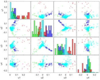
FIGURE 1 : Plot of the community structure in the space spanned by the top

four left singular vectors. Here each color represents a community

and ui,1 ≤ i ≤ 4 denotes the singular vectors respectively. For

instance, the top right subfigure denotes projecting the nodes onto

the space spanned by (u4, u1). . . 2

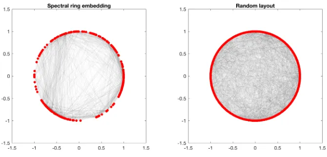
FIGURE 2 : Plot of the ring lattice structure. On the left, the layout is returned

by our spectral embedding algorithm; on the right, the layout is

returned by a random permutation. . . 3

FIGURE 3 : Simulated neuron data with three fitting models: cubic smoothing

spline, polynomial regression of degree 4, and Bayesian adaptive

regression splines (BARS). . . 4

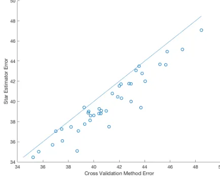
FIGURE 4 : Plot of MSE of Star algorithm compared to cross validation. . . 4

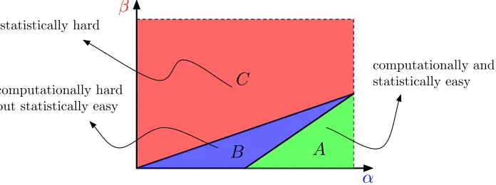
FIGURE 5 : Phase diagram for submatrix localization. Red region (C):

statis-tically impossible, where even without computational budget, the

problem is hard. Blue region (B): statistically possible but

compu-tationally expensive (under the hidden clique hypothesis), where

the problem is hard to all polynomial time algorithm but easy with

exponential time algorithm. Green region (A): statistically possible

and computationally easy, where a fast polynomial time algorithm

will solve the problem. . . 13

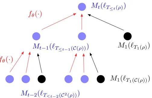
FIGURE 7 : Illustration of recursion in Eq. (2.14) for messages on a d-regular

tree. Hered= 3 with two unlabeled children ((1₋δ)d= 2, denoted

by blue) and one labeled child (δd= 1, denoted by black), and the

depth is 2. Ct_{(ρ) denotes depth t children of the root ρ. The red}

arrows correspond to messages received from the labeled children

and black arrow are from the unlabeled children. . . 45

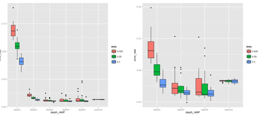
FIGURE 8 : AMP algorithm on Political Blog Dataset. . . 57

FIGURE 9 : Phase diagram for small-world network: impossible region (red

re-gion I), hard rere-gion (blueregion II), easy region (greenregion III),

and reconstructable region (cyanregion IV). . . 63

FIGURE 10 : Phase diagram for small-world networks: impossible region (red

re-gion I), hard rere-gion (blueregion II), easy region (greenregion III),

and reconstructable region (cyan region IV and IV’). Compared

to Figure 9, the spectral ordering procedure extends the

recon-structable region (IV) whenkn1516 (IV’). . . 72

FIGURE 11 : Ring embedding of Les Mis´erable co-appearance network. . . 73

FIGURE 12 : The structural matrices for stochastic block model (left), mixed

membership SBM (middle), and small-world model (right). The

black location denotes the support of the structural matrix. . . . 74

FIGURE 13 : Proof of the geometry inequality. The solid and dotted balls are

B(Y,kbg−Ykn) and B(Y,kfb−Ykn), respectively. . . 80

FIGURE 14 : Tangent cone: general illustration in 2D. The red shaped area is

the scaled convex hull of atom set. The blue dashed line forms the

tangent cone at M. Black arrow denotes the possible directions

inside the cone. . . 104

FIGURE 15 : Tangent cone illustration in 3D for sparse regression. For three

possible locations Mi,1 ≤ i ≤ 3, the tangent cone are different,

CHAPTER 1 : Introduction

The unprecedented “data deluge” emerging in science and engineering in recent years poses

many challenges to the development of theory and methodology. Specifically, part of the

new features of these challenges can be summarized as follows:

• Inference How to make inference on a large amount of unknown variables or

param-eters with limited amount of partial, noisy, and indirect measurements (observations)?

• Learning How to predict as well as a class of complex models (non-linear and

non-convex), using heterogeneous data that can be arbitrary or even adversarial, in

various specific protocols (online, bandit feedback, partial information)?

• Computation Computation adds a new dimension to this modern challenge. As

the scale of the data increases significantly, how to take computational and memory

budgets into account when designing inference and learning algorithms?

The goal of this thesis is to investigate these features for two collections of problems:

statis-tical network inference, and model selection in regression. We will start with two concrete

data examples as a gentle introduction to motivate our studies, then we will move to the

outline of the remaining chapters before stepping into detailed discussions.

Structural inference of C. elegans neuron network In this paragraph, we will use

the C. elegans neuron network (Pavlovic et al., 2014) as an example to illustrate the

im-portance of structural inference for complex networks, which is the focus of Chapter 2. C.

elegans is one of the simplest organisms with a nervous system whose neuronal “wiring

diagram” (neural connections) has been completed (with around 300 neurons and 2000

edges). In practice, it is important to understand the structural information of the complex

systems/networks based on the connection patterns. From the statistical side, researchers

often model the network as generated from some statistical model (for example, stochastic

structure from the data. Brute-force maximum likelihood based approach is usually

com-putationally prohibitive with large scale networks. Therefore, it is important to understand

when we can solve the inference problem in a computationally efficient manner. Here we

illustrate some of the methods proposed in Chapter 2 on this C.elegans network.

We apply the algorithm proposed in Chapter 2.1 on discovering the community structure

on this dataset. Figure 1 summarizes the community structure we discover.

Figure 1: Plot of the community structure in the space spanned by the top four left singular vectors. Here each color represents a community and ui,1 ≤ i ≤ 4 denotes the singular vectors respectively. For instance, the top right subfigure denotes projecting the nodes onto the space spanned by (u4, u1).

We also apply the algorithm proposed in Chapter 2.3 on reconstructing the ring lattice

structure on this dataset. Figure 2 describes the result. On the left, we solve for the ring

the nodes. On the right, we randomly permute the nodes as the circle layout (what one

expects to see without the ring lattice structure). As a contrast, one can clearly see the

edges are much better organized in the left compared to the right, suggesting the presence

of Watts-Strogatz ring lattice structure.

Figure 2: Plot of the ring lattice structure. On the left, the layout is returned by our spectral embedding algorithm; on the right, the layout is returned by a random permutation.

Model selection for fitting neuronal data In this paragraph, we will employ simulated

neuronal data (Kaufman et al., 2005) to motivate the focus of Chapter 3 — model selection

in regression. The task is to predict the firing rate of neurons based on the simulated data as

good as the best one among a collection of models. Specifically, in Figure 3, we fitted three

models, cubic smoothing spline, polynomial regression of degree 4, and Bayesian adaptive

regression splines (BARS). Traditionally, model selection is typically addressed using

cross-validation (CV) in a general way. However, it is questionable whether CV will provide

the optimal behavior, let alone the computational burden when facing a large collection of

Figure 3: Simulated neuron data with three fitting models: cubic smoothing spline, poly-nomial regression of degree 4, and Bayesian adaptive regression splines (BARS).

We apply the two-step Star algorithm proposed in Chapter 3.1 on the neuronal dataset,

and summarize the result in Figure 4. Here each data point corresponds to one experiment,

whose x-axis denotes the mean square error (MSE) of the cross-validation, and y-axis

de-notes the MSE of the Star algorithm. As one can see, clearly the Star algorithm outperforms

the CV significantly over many experiments.

1.1. Outline

1.1.1. Chapter 2

Historically, statisticians and information theorists mostly focus on analyzing the threshold

that separates “signal” and “noise” over random instances (in the average-case sense),

over-looking computation complexity. However, computer scientists are usually concerned with

quantifying problems according to their computational difficulty in the worst-case sense. In

this chapter, we will investigate the intersection of the above perspectives. For an average

instance, we would like to: (a) identify the statistical threshold that describes the solvability

of the problem information-theoretically, and (b) quantify the computational threshold that

sheds light on the difficulty for polynomial-time algorithms (inside the statistically solvable

phase).

In Cai et al. (2015a), we examined the above two thresholds on the problem of

subma-trix localization with background noise. We discovered that, quite surprisingly, there is

always an intrinsic gap between computational and statistical thresholds under standard

computational hardness assumption. There is a non-vanishing phase quantifying the price

to pay for pursuing polynomial run-time. We established the computational optimality in

two stages: (a) we provided a new average-case reduction to the hidden clique problem; (b)

we proposed a simple near-linear time algorithm that achieves the computational threshold.

Overall, this work illustrates that for certain statistical problems, there are more structured

phases inside the statistically-solvable phase.

Motivated by the fact that real network datasets always contain side information (partial

labels, nodes’ features) in addition to the connections, our work Cai et al. (2016c) studied

the computational difficulty of partially-labeled stochastic block models when a vanishing

portion of true labels are revealed. One the one hand, we derived and analyzed a new

lo-cal algorithm — linearized message passing — that achieves exponential decaying error for

we proved that this K-S threshold is indeed the barrier for all local algorithms

(heuristi-cally believed to be powerful polynomial time algorithms) through a minimax lower bound.

Whether the gap between K-S and information-theoretic threshold (with growing number

of blocks) is inevitable for polynomial time algorithms, remains an open problem.

In Cai et al. (2016a), we initiated the investigation of the corresponding thresholds for

detec-tion and structural reconstrucdetec-tion in Watts-Strogatz (W-S) small world networks. The W-S

model with neighborhood size kand rewiring probability β can be viewed as a continuous

interpolation between a deterministic ring lattice graph and the Erd˝os-R´enyi random graph.

We studied both the computational and statistical aspects of detecting the deterministic

ring lattice structure (or local geographical links) in the presence of random connections (or

long range links), and for its recovery. We partitioned parameter space (k, β) into several

phases according to the difficulty of the problem, and proposed distinct methods that

math-ematically achieve the corresponding thresholds separating the phases. We implemented our

spectral ring embedding algorithm on the Les Mis´erables co-appearance network.

1.1.2. Chapter 3

In this chapter we will study regression and model selection problem focusing on two aspects:

(a) model misspecification; (b) model class can be non-convex. For the first point, classic

decision theory is concerned with making decisions from i.i.d. data generated from a

well-specified statistical model. However, one should be agnostic about these two assumptions:

(a) the i.i.d. data may be generated from a mis-specified model; (b) the underlying stochastic

process generating the data is non-i.i.d., even adversarially chosen by oblivious nature.

Statistical learning theory and online learning provide handful tools to solve these two

problems respectively. For the second point, when the model class is non-convex (such as

sparse linear regression and finite aggregation), we would like to understand its consequences

on the estimation/prediction procedure and accuracy, as well as the computation difficulty.

learning setting (i.i.d., mis-specified model), for general classes of functions that can be

unbounded and non-convex. We introduced a new notion of offset Rademacher complexity,

and showed that the excess loss can be upper bounded by this new complexity through a

novel geometric inequality. We achieved this goal through: (a) proposing a novel two-step

estimator; (b) adopting the symmetrization and chaining tools in empirical processes theory

to this offset complexity. We showed that localization for unbounded class is automatic

through this offset analysis. This new framework recovers the sharp rates in parametric

regression, finite aggregation, and non-parametric regression simultaneously.

Cai et al. (2016b) presents a unified geometric framework for the statistical analysis of a

general ill-posed linear inverse model which includes as special cases noisy compressed

sens-ing, sign vector recovery, trace regression, orthogonal matrix estimation, and noisy matrix

completion. We propose computationally feasible convex programs for statistical inference

including estimation, confidence intervals and hypothesis testing. A theoretical framework

is developed to characterize the local estimation rate of convergence and to provide

sta-tistical inference guarantees. Our results are built based on the local conic geometry and

duality. The difficulty of statistical inference is captured by the geometric characterization

of the local tangent cone through the Gaussian width and Sudakov estimate.

Online sparse linear regression is an online problem where an algorithm repeatedly chooses

a subset of coordinates to observe in an adversarially chosen feature vector, makes a

real-valued prediction, receives the true label, and incurs the squared loss. The goal is to design

an online learning algorithm with sublinear regret to the best sparse linear predictor in

hind-sight. Without any assumptions, this problem is known to be computationally intractable.

In Kale et al. (2017), we make the assumption that data matrix satisfies restricted

isome-try property, and show that this assumption leads to computationally efficient algorithms

with sublinear regret for two variants of the problem. In the first variant, the true label is

generated according to a sparse linear model with additive Gaussian noise. In the second,

CHAPTER 2 : Statistical Network Inference and Computation

2.1. Submatrix Localization and Bi-Clustering

2.1.1. Introduction

The “signal + noise” model

X=M+Z, (2.1)

where M is the signal of interest and Z is noise, is ubiquitous in statistics and is used

in a wide range of applications. Such a “signal + noise” model has been well studied

in statistics in a number of settings, including nonparametric regression where M is a

function, and the Gaussian sequence model where M is a finite or an infinite dimensional

vector. See, for example, Tsybakov (2009); Johnstone (2013) and the references therein.

In nonparametric regression, the structural knowledge on M is typically characterized by

smoothness, and in the sequence model the structural knowledge on M is often described

by sparsity. Fundamental statistical properties such as the minimax estimation rates and

the signal detection boundaries have been established under these structural assumptions.

For a range of contemporary applications in statistical learning and signal processing,M and

Z in the “signal + noise” model (2.1) are high-dimensional matrices (Tufts and Shah, 1993;

Drineas et al., 2006; Donoho and Gavish, 2014; Chandrasekaran et al., 2009; Cand`es et al.,

2011). In this setting, many new interesting problems arise under a variety of structural

assumptions onM and the distribution ofZ. Examples include sparse principal component

analysis (PCA) (Vu and Lei, 2012; Berthet and Rigollet, 2013b; Birnbaum et al., 2013;

Cai et al., 2013, 2015b), low-rank matrix de-noising (Donoho and Gavish, 2014), matrix

factorization and decomposition (Chandrasekaran et al., 2009; Cand`es et al., 2011; Agarwal

et al., 2012), non-negative PCA (Zass and Shashua, 2006; Montanari and Richard, 2014),

synchronization and planted partition (Javanmard et al., 2015; Decelle et al., 2011), among

many others. In the conventional statistical framework, the goal is developing optimal

statistical procedures (for estimation, testing, etc), where optimality is understood with

respect to the sample size and parameter space.

When the dimensionality of the data becomes large as in many contemporary applications,

the computational concerns associated with the statistical procedures come to the

fore-front. After all, statistical methods are useful in practice only if they can be computed

within a reasonable amount of time. A fundamental question is: Is there a price to pay

for statistical performance if one only considers computable (polynomial-time) procedures?

This question is particularly relevant for non-convex problems with combinatorial

struc-tures. These problems pose a significant computational challenge because naive methods

based on exhaustive search are typically not computationally efficient. Trade-off between

computational efficiency and statistical accuracy in high-dimensional inference has drawn

increasing attention in the literature. In particular, Chandrasekaran et al. (2012) and

Wain-wright (2014) considered a general class of linear inverse problems, with different emphasis

on geometry of convex relaxation and decomposition of statistical and computational

er-rors. Chandrasekaran and Jordan (2013) studied an approach for trading off computational

demands with statistical accuracy via relaxation hierarchies. Berthet and Rigollet (2013a);

Ma and Wu (2013a); Zhang et al. (2014b) focused on computational difficulties for various

statistical problems, such as detection and regression.

In the present thesis, we study the interplay between computational efficiency and statistical

accuracy in submatrix localization based on a noisy observation of a large matrix. The

Problem Formulation

Consider the matrix X of the form

X=M+Z, where M =λ_·1Rm1 T

Cn (2.2)

and 1Rm ∈R

m_{denotes a binary vector with 1 on the index setR}

mand zero otherwise. Here,

the entriesZij of the noise matrix are i.i.d. zero-mean sub-Gaussian random variables with

parameterσ (defined formally in Equation (2.5)). Given the parameters m, n, km, kn, λ/σ,

the set of all distributions described above – for all possible choices ofRm and Cn – forms

the submatrix model _M(m, n, km, kn, λ/σ).

This model can be further extended to multiple submatrices where

M =

r

X

s=1

λs·1Rs1 T

Cs (2.3)

where _|Rs| = ks(m) and |Cs| = ks(n) denote the support set of the s-th submatrix. For

simplicity, we first focus on the single submatrix and then extend the analysis to the model

(2.3) in Section 2.1.2.

There are two fundamental questions associated with the submatrix model (2.2). One is the

detection problem: given one observation of the X matrix, decide whether it is generated

from a distribution in the submatrix model or from the pure noise model. Precisely, the

detection problem considers testing of the hypotheses

H0 :M =0 v.s. Hα :M ∈ M(m, n, km, kn, λ/σ).

The other is thelocalization problem, where the goal is to exactly recover the signal index

setsRmandCn(the support of the mean matrixM). It is clear that the localization problem

focus of the current thesis is on the localization problem. As we will show in this thesis,

the localization problem requires larger signal to noise ratio, as well as novel algorithm and

analysis to exploit the submatrix structure.

Main Results

To state our main results, let us first define a hierarchy of algorithms in terms of their

worst-case running time on instances of the submatrix localization problem:

LinAlg⊂PolyAlg⊂ExpoAlg⊂AllAlg.

The setLinAlgcontains algorithmsA that produce an answer (in our case, the localization

subset ˆRA

m,CˆnA) in time linear inm×n(the minimal computation required to read the

ma-trix). The classesPolyAlgandExpoAlg of algorithms, respectively, terminate in polynomial

and exponential time, whileAllAlg has no restriction.

Combining Theorem 2.1.3 and 2.1.4 in Section 2.1.2 and Theorem 2.1.5 in Section 2.1.3,

the statistical and computational boundaries for submatrix localization can be summarized

as follows. The notations %,-,are formally defined in Section 2.1.1.

Theorem 2.1.1 (Computational and Statistical Boundaries). Consider the submatrix

lo-calization problem under the model (2.2). The computational boundary SNRc for the dense

case when min_{km, kn}%max{m1/2, n1/2} is

SNRc

r

m∨n

kmkn +

r logn

km ∨

logm kn

,

in the sense that

lim m,n,km,kn→∞

inf

A∈LinAlg _Msup∈MP

ˆ

R_mA 6=Rm or CˆnA 6=Cn

= 0, if λ

σ %SNRc

lim m,n,km,kn→∞

inf

A∈PolyAlg _Msup_∈MP

ˆ

RA_m6=Rm or CˆnA6=Cn

>0, if λ

where (2.4)holds under the Hidden Clique hypothesis HCl(see Section 2.1.2). For the sparse

case when max_{km, kn} -min{m1/2, n1/2}, the computational boundary is SNRc= Θ∗(1),

more precisely

1-SNRc

-r

logm∨n

kmkn

.

The statistical boundary SNRs is

SNRs

r logn

km ∨

logm kn

,

in the sense that

lim m,n,km,kn→∞

inf

A∈ExpoAlg _Msup∈MP

ˆ

RA_m6=Rm or CˆnA6=Cn

= 0, if λ

σ %SNRs

lim m,n,km,kn→∞

inf

A∈AllAlg _Msup_∈MP

ˆ

RA_m6=Rm or CˆnA6=Cn

>0, if λ

σ -SNRs

under the minimal assumption max{km, kn}-min{m, n}.

If we parametrize the submatrix model as m=n, km knk= Θ∗(nα), λ/σ = Θ∗(n−β),

for some 0< α, β <1, we can summarize the results of Theorem 2.1.1 in a phase diagram,

as illustrated in Figure 5.

To explain the diagram, consider the following cases. First, the statistical boundary is

r logn

km ∨

logm kn

,

which gives the line separating the red and the blue regions. For the dense regimeα_≥1/2,

the computational boundary given by Theorem 2.1.1 is

r

m_∨n

kmkn +

r logn

km ∨

logm kn

,

↵

computationally and statistically easy computationally hard

but statistically easy statistically hard

B

A

C

Figure 5: Phase diagram for submatrix localization. Red region (C): statistically impos-sible, where even without computational budget, the problem is hard. Blue region (B): statistically possible but computationally expensive (under the hidden clique hypothesis), where the problem is hard to all polynomial time algorithm but easy with exponential time algorithm. Green region (A): statistically possible and computationally easy, where a fast polynomial time algorithm will solve the problem.

regime α < 1/2, the computational boundary is Θ(1) -SNRc - Θ(

q

log m∨n

kmkn), which is

the horizontal line connecting (α= 0, β= 0) to (α= 1/2, β= 0).

As a key part of Theorem 2.1.1, we provide linear time spectral algorithm that will succeed

in localizing the submatrix with high probability in the regime above the computational

threshold. Furthermore, the method is data-driven and adaptive: it does not require the

prior knowledge on the size of the submatrix. This should be contrasted with the method of

Chen and Xu (2014) which requires the prior knowledge ofkm, kn; furthermore, the running

time of their SDP-based method is superlinear innm. Under the hidden clique hypothesis,

we prove that below the computational threshold there is no polynomial time algorithm

that can succeed in localizing the submatrix. We remark that the computational lower

bound for localization requires distinct new techniques compared to the lower bound for

detection; the latter has been resolved in Ma and Wu (2013a).

Beyond localization of one single submatrix, we generalize both the computational and

sta-tistical story to a growing number of submatrices in Section 2.1.2. As mentioned earlier, the

culty of localization for a growing number of submatrices, at the expense of not providing

the exact constants for the thresholds.

The phase transition diagram in Figure 5 for localization should be contrasted with the

corresponding result for detection, as shown in (Butucea and Ingster, 2013; Ma and Wu,

2013a). For a large enough submatrix size (as quantified byα >2/3), the

computationally-intractable-but-statistically-possible region collapses for the detection problem, but not for

localization. In plain words, detecting the presence of a large submatrix becomes both

computationally and statistically easy beyond a certain size, while for localization there

is always a gap between statistically possible and computationally feasible regions. This

phenomenon also appears to be distinct to that of other problems like estimation of sparse

principal components (Cai et al., 2013), where computational and statistical easiness

coin-cide with each other over a large region of the parameter spaces.

Prior Work

There is a growing body of work in statistical literature on submatrix problems.

Arias-Castro et al. (2011) studied the detection problem for a cluster inside a large matrix.

Butucea and Ingster (2013); Butucea et al. (2013) formulated the submatrix detection

and localization problems under Gaussian noise and determined sharp statistical transition

boundaries. For the detection problem, Ma and Wu (2013a) provided a computational lower

bound result under the assumption that hidden clique detection is computationally difficult.

Shabalin et al. (2009) provided a fast iterative maximization algorithm to heuristically solve

the submatrix localization problem. Balakrishnan et al. (2011); Kolar et al. (2011) focused

on statistical and computational trade-offs for the submatrix localization problem. Under

the sparse regimekm -m1/2 andkn-n1/2, the entry-wise thresholding turns out to be the

“near optimal” polynomial-time algorithm (which we will show to be a de-noised spectral

algorithm that perform slightly better in Section 2.1.2). However, for the dense regime when

in the sense that there are other polynomial-time algorithm that can succeed in finding the

submatrix with smaller SNR. Concurrently with our work, Chen and Xu (2014) provided a

convex relaxation algorithm that improves the SNR boundary of Kolar et al. (2011) in the

dense regime. On the computational downside, the implementation of the method requires

a full SVD on each iteration, and therefore does not scale well with the dimensionality

of the problem. Furthermore, there is no computational lower bound in the literature to

guarantee the optimality of the SNR boundary achieved in Chen and Xu (2014). A problem

similar to submatrix localization is that of clique finding in random graph. Deshpande and

Montanari (2013) presented an iterative approximate message passing algorithm to solve

the latter problem with sharp boundaries on SNR.

We would like to emphasize on the differences between the localization and the

detec-tion problems. In terms of the theoretical results, unlike detecdetec-tion, there is always a gap

between statistically optimal and computationally feasible regions for localization. This

non-vanishing computational-to-statistical-gap phenomenon also appears in the community

detection literature with growing number of communities (Decelle et al., 2011). In terms of

the methodology, for detection, combining the results in (Donoho and Jin, 2004; Ma and

Wu, 2013a), there is no loss in treating M in model (2.2) as a vector and applying the

higher criticism method (Donoho and Jin, 2004) to the vectorized matrix for the problem of

submatrix detection, in the computationally efficient region. In fact, the procedure achieves

sharper constants in the Gaussian setting. However, in contrast, we will show that for

lo-calization, it is crucial to utilize the matrix structure, even in the computationally efficient

region.

Organization

The section is organized as follows. Section 2.1.2 establishes the computational boundary,

with the computational lower bounds given in Section 2.1.2 and upper bound results in

2.1.2. The upper and lower bounds for statistical boundary for multiple submatrices are

discussed in Section 2.1.3. A short discussion is given in Section 2.1.4. Technical proofs are

deferred to Appendix.

Notation

Let [m] denote the index set{1,2, . . . , m}. For a matrix X ∈Rm×n,Xi· ∈Rn denotes its

i-th row andX·j ∈Rm denotes itsj-th column. For any I ⊆[m], J ⊆[n], XIJ denotes the

submatrix corresponding to the index setI_×J. For a vectorv_∈Rn,kvk`p = ( P

i∈[n]|vi|p)1/p

and for a matrix M _∈ Rm×n, kMk`p = supv=6 0kM vk`p/kvk`p. When p = 2, the latter is

the usual spectral norm, abbreviated as_kM_k2. The nuclear norm of a matrixM is convex

surrogate for the rank, with the notation to be_kM_k∗. The Frobenius norm of a matrixM

is defined as _kM_kF =

q P

i,jMij2. The inner product associated with the Frobenius norm

is defined as hA, Bi=tr(AT_B).

Denote the asymptotic notationa(n) = Θ(b(n)) if there exist two universal constantscl, cu

such that cl ≤ lim

n→∞a(n)/b(n)≤nlim→∞a(n)/b(n) ≤cu. Θ

∗ _{is asymptotic equivalence hiding}

logarithmic factors in the following sense: a(n) = Θ∗_{(b(n)) iff there exists c >0 such that}

a(n) = Θ(b(n) logc_{n). Additionally, we use the notationa(n)b(n) as equivalent toa(n) =}

Θ(b(n)), a(n)%b(n) iff limn→∞a(n)/b(n) =∞ anda(n)-b(n) iff limn→∞a(n)/b(n) = 0.

We define the zero-mean sub-Gaussian random variable z with sub-Gaussian parameter σ

in terms of its Laplacian

Eeλz≤exp(σ2λ2/2), for all λ >0, (2.5)

then we have

We call a random vectorZ _∈Rn isotropic with parameterσ if

E(vTZ)2 =σ2kvk2`2, for all v∈R

n_.

Clearly, Gaussian and Bernoulli measures, and more general product measures of zero-mean

sub-Gaussian random variables satisfy this isotropic definition up to a constant scalar factor.

2.1.2. Computational Boundary

We characterize in this section the computational boundaries for the submatrix localization

problem. Sections 2.1.2 and 2.1.2 consider respectively the computational lower bound and

upper bound. The computational lower bound given in Theorem 2.1.2 is based on the

hidden clique hypothesis.

Algorithmic Reduction and Computational Lower Bound

Theoretical Computer Science identifies a range of problems which are believed to be “hard,”

in the sense that in the worst-case the required computation grows exponentially with the

size of the problem. Faced with a new computational problem, one might try to reduce any

of the “hard” problems to the new problem, and therefore claim that the new problem is

as hard as the rest in this family. Since statistical procedures typically deal with a random

(rather than worst-case) input, it is natural to seek token problems that are believed to be

computationally difficult on average with respect to some distribution on instances. The

hidden clique problem is one such example (for recent results on this problem, see Feldman

et al. (2013); Deshpande and Montanari (2013)). While there exists a quasi-polynomial

algorithm, no polynomial-time method (for the appropriate regime, described below) is

known. Following several other works on reductions for statistical problems, we work under

the hypothesis that no polynomial-time method exists.

Let us make the discussion more precise. Consider the hidden clique modelG(N, κ) where

model, a random graph instance is generated in the following way. Choose κ clique nodes

uniformly at random from all the possible choices, and connect all the edges within the

clique. For all the other edges, connect with probability 1/2.

Hidden Clique Hypothesis for Localization (HCl) Consider the random instance

of hidden clique model G(N, κ). For any sequence κ(N) such that κ(N) ≤ Nβ _{for some}

0< β <1/2, there is no randomized polynomial time algorithm that can find the planted

clique with probability tending to 1 as N _{→ ∞}. Mathematically, define the randomized

polynomial time algorithm class PolyAlgas the class of algorithms_A that satisfies

lim

N,κ(N)→∞A∈supPolyAlgE

CliquePG(N,κ)|Clique(runtime of A not polynomial inN) = 0.

Then

lim N,κ(N)→∞

inf

A∈PolyAlgECliquePG(N,κ)|Clique(clique set returned by Anot correct)>0,

where PG(N,κ)|Clique is the (possibly more detailed due to randomness of algorithm) σ-field

conditioned on the clique location and EClique is with respect to uniform distribution over

all possible clique locations.

Hidden Clique Hypothesis for Detection (HCd) Consider the hidden clique model

G(N, κ). For any sequence ofκ(N) such thatκ(N)≤Nβ _{for some 0< β <1/2, there is no}

randomized polynomial time algorithm that can distinguish between

H0 : PER v.s. Hα: PHC

with probability going to 1 as N → ∞. Here PER is the Erd˝os-R´enyi model, while PHC is

More precisely,

lim N,κ(N)→∞

inf

A∈PolyAlgECliquePG(N,κ)|Clique(detection decision returned by Awrong)>0,

wherePG(N,κ)|Clique andEClique are the same as defined in HCl.

The hidden clique hypothesis has been used recently by several authors to claim

compu-tational intractability of certain statistical problems. In particular, Berthet and Rigollet

(2013a); Ma and Wu (2013a) assumed the hypothesis HCd and Wang et al. (2014) used

HCl. Localization is harder than detection, in the sense that if an algorithm A solves the

localization problem with high probability, it also correctly solves the detection problem.

Assuming that no polynomial time algorithm can solve the detection problem implies

im-possibility results in localization as well. In plain language,HCl is a milder hypothesis than

HCd.

We will provide computational lower bound result for localization in Theorem 2.1.2. In

Appendix, we contrast the difference of lower bound constructions between localization and

detection. The detection computational lower bound was proved in Ma and Wu (2013a).

For the localization computational lower bound, to the best of our knowledge, there is no

proof in the literature. Theorem 2.1.2 ensures the upper bound in Lemma 2.1.1 being sharp.

Theorem 2.1.2 (Computational Lower Bound for Localization). Consider the submatrix

model (2.2) with parameter tuple (m = n, km kn nα, λ/σ = n−β), where 1₂ < α <

1, β >0. Under the computational assumption HCl, if

λ

σ

-r

m+n

kmkn ⇒

β > α−1

2,

it is not possible to localize the true support of the submatrix with probability going to 1

within polynomial time.

the usual computational lower bound arguments. Bootstrapping introduces an additional

randomness on top of the randomness in the hidden clique. Careful examination of these

two σ-fields allows us to write the resulting object into mixture of submatrix models. For

submatrix localization we need to transform back the submatrix support to the original

hidden clique support exactly, with high probability. In plain language, even though we

lose track of the exact location of the support when reducing the hidden clique to submatrix

model, we can still recover the exact location of the hidden clique with high probability.

For technical details of the proof, please refer to the Appendix.

Adaptive Spectral Algorithm and Upper Bound

In this section, we introduce linear time algorithm that solves the submatrix localization

problem above the computational boundary SNRc. Our proposed localization Algorithms

1 and 2 are motivated by the spectral algorithm in random graphs (McSherry, 2001; Ng

et al., 2002).

Algorithm 1 Vanilla Spectral Projection Algorithm for Dense Regime Input: X_∈Rm×n the data matrix.

Output: A subset of the row indexes ˆRm and a subset of column indexes ˆCn as the

local-ization sets of the submatrix.

1. Compute top left and top right singular vectorsU·1andV·1, respectively (these correspond

to the SVDX =UΣVT₎

2. To compute ˆCn, calculate the inner productsU·T1X·j ∈R,1≤j≤n. These values form

two data-driven clusters, and a cut at the largest gap between consecutive values returns

the subsets ˆCn and [n]\Cˆn. Similarly, for the ˆRm, calculate Xi·V·1 ∈ R,1 ≤ i ≤ m and

obtain two separated clusters.

The proposed algorithm has several advantages over the localization algorithms that

ap-peared in literature. First, it is a linear time algorithm (that is, Θ(mn) time complexity).

ef-ficient both in terms of space and time. Secondly, this algorithm does not require the prior

knowledge of km and kn and automatically adapts to the true submatrix size.

Lemma 2.1.1 below justifies the effectiveness of the spectral algorithm.

Lemma 2.1.1 (Guarantee for Spectral Algorithm). Consider the submatrix model (2.2),

Algorithm 1 and assume min{km, kn} % max{m1/2, n1/2}. There exist a universal C > 0

such that when

λ

σ ≥C·

r

m_∨n

kmkn +

r logn

km ∨

logm kn

! ,

the spectral method succeeds in the sense that Rˆm =Rm,Cˆn =Cn with probability at least

1₋m−c_−n−c_{−2 exp (−c(m+n)).}

Remark 2.1.1. The theory and algorithm remain the same if the signal matrixM is more

general in the following sense: M has rank one, its left and right singular vectors are sparse,

and the nonzero entries of the singular vectors are of the same order. Mathematically,

M = λ√kmkn·uvT, where u, v are unit singular vectors with km, kn non-zero entries,

and |u|max/|u|min ≤ c and |v|max/|v|min ≤ c for some constant c ≥ 1. Here for a vector

w, |w|max and |w|min denote respectively the largest and smallest magnitudes among the

nonzero coordinates. When c = 1, the algorithm is fully data-driven and does not require

the knowledge of λ, σ, km, kn. When c is large but finite, one may require in addition the

knowledge of km and kn to perform the final cut to obtain ˆCn and ˆRm.

Dense Regime

We are now ready to state the SNR boundary for polynomial-time algorithms (under an

appropriate computational assumption), thus excluding the exhaustive search procedure.

The results hold under the dense regime when k%n1/2_.

Theorem 2.1.3 (Computational Boundary for Dense Regime). Consider the submatrix

model (2.2)and assume min{km, kn}%max{m1/2, n1/2}. There exists a critical rate

SNRc

r

m_∨n

k k +

r logn

k ∨

for the signal to noise ratio SNRc such that for λ/σ % SNRc, both the adaptive linear

time Algorithm 1 and convex relaxation (runs in polynomial time) will succeed in submatrix

localization, i.e., Rˆm =Rm,Cˆn = Cn, with high probability. For λ/σ -SNRc, there is no

polynomial time algorithm that will work under the hidden clique hypothesis HCl.

The proof of the above theorem is based on the theoretical justification of the spectral

Algorithm 1 and the new computational lower bound result for localization in Theorem

2.1.2. We remark that the analyses can be extended to multiple, even growing number of

submatrices case. We postpone a proof of this fact to Section 2.1.2 for simplicity and focus

on the case of a single submatrix.

Sparse Regime

Under the sparse regime whenk-n1/2_{, a naive plug-in of Lemma 2.1.1 requires theSNR}

c

to be larger than Θ(n1/2_{/k) %} √_{logn, which implies the vanilla spectral Algorithm 1 is}

outperformed by simple entrywise thresholding. However, a modified version with

entry-wise soft-thresholding as a preprocessing de-noising step turns out to provide near optimal

performance in the sparse regime. Before we introduce the formal algorithm, let us define

the soft-thresholding function at level tto be

ηt(y) = sign(y)(|y| −t)+. (2.6)

Soft-thresholding as a de-noising step achieving optimal bias-and-variance trade-off has been

widely understood in the wavelet literature, for example, see Donoho and Johnstone (1998).

Now we are ready to state the following de-noised spectral Algorithm 2 to localize the

Algorithm 2 De-noised Spectral Algorithm for Sparse Regime

Input: X_∈Rm×n the data matrix, a thresholding level t= Θ(σ

q

log m∨n kmkn).

Output: A subset of the row indexes ˆRm and a subset of column indexes ˆCn as the

local-ization sets of the submatrix.

1. Soft-threshold each entry of the matrix X at level t, denote the resulting matrix as

ηt(X)

2. Compute top left and top right singular vectorsU·1 andV·1 of matrixηt(X), respectively

(these correspond to the SVDηt(X) =UΣVT)

3. To compute ˆCn, calculate the inner products U·T1 ·ηt(X·j),1 ≤ j ≤ n. These values

form two clusters. Similarly, for the ˆRm, calculate ηt(Xi·)·V·1,1≤i≤m and obtain two

separated clusters. A simple thresholding procedure returns the subsets ˆCn and ˆRm.

Lemma 2.1.2 below provides the theoretical guarantee for the above algorithm when k

-n1/2_.

Lemma 2.1.2 (Guarantee for De-noised Spectral Algorithm). Consider the submatrix

model (2.2), soft-thresholded spectral Algorithm 2 with thresholded level σt, and assume

min_{km, kn}-max{m1/2, n1/2}. There exist a universal C >0 such that when

λ

σ ≥C·

"_r

m∨n

kmkn +

r logn

km ∨

logm kn

#

·e−t2/2+t !

,

the spectral method succeeds in the sense that Rˆm =Rm,Cˆn =Cn with probability at least

1−m−c_−n−c_{−2 exp (−c(m+n)). Further if we choose Θ(σ}q_log m∨n

kmkn) as the optimal

thresholding level, we have de-noised spectral algorithm works when

λ

σ %

r

logm∨n

kmkn

.

Combining the hidden clique hypothesis HCl together with Lemma 2.1.2, the following

Theorem 2.1.4 (Computational Boundary for Sparse Regime). Consider the submatrix

model (2.2) and assume max_{km, kn} - min{m1/2, n1/2}. There exists a critical rate for

the signal to noise ratioSNRc between

1-SNRc

-r

logm∨n

kmkn

such that for λ/σ % qlog m∨n

kmkn, the linear time Algorithm 2 will succeed in submatrix

localization, i.e., Rˆm = Rm,Cˆn = Cn, with high probability. For λ/σ - 1, there is no

polynomial time algorithm that will work under the hidden clique hypothesis HCl.

Remark 2.1.2. The upper bound achieved by the de-noised spectral Algorithm 2 is optimal

in the two boundary cases: k= 1 andkn1/2_{. Whenk= 1, both the information theoretic}

and computational boundary meet at √logn. When k n1/2_{, the computational lower}

bound and upper bound match in Theorem 2.1.4, thus suggesting the near optimality of

Algorithm 2 within the polynomial time algorithm class. The potential logarithmic gap is

due to the crudeness of the hidden clique hypothesis. Precisely, for k = 2, hidden clique

is not only hard for G(n, p) with p = 1/2, but also hard for G(n, p) with p = 1/logn.

Similarly for k=nα_{, α <1/2, hidden clique is not only hard for G(n, p) with p= 1/2, but}

also for some 0< p <1/2.

Extension to Growing Number of Submatrices

The computational boundaries established in the previous sections for a single submatrix

can be extended to non-overlapping multiple submatrices model (2.3). The non-overlapping

assumption corresponds to that for any 1≤s6=t≤r,Rs∩Rt=∅ and Cs∩Ct=∅. The

Algorithm 3 below is an extension of the spectral projection Algorithm 1 to address the

Algorithm 3 Spectral Algorithm for Multiple Submatrices

Input: X_∈Rm×n the data matrix. A pre-specified number of submatrices r.

Output: A subset of the row indexes _{Rˆs

m,1 ≤ s ≤ r} and a subset of column indexes

{Cˆs

n,1≤s≤r} as the localization of the submatrices.

1. Calculate top r left and right singular vectors in the SVD X = UΣVT_{. Denote these}

vectors as Ur∈Rm×r and Vr ∈Rn×r, respectively

2. For the ˆCs

n,1 ≤s ≤ r, calculate the projection Ur(UrTUr)−1UrTX·j,1 ≤ j ≤ n, run k

-means clustering algorithm (withk=r+1) for thesenvectors inRm. For the ˆRsm,1≤s≤r,

calculateVr(VrTVr)−1VrTXiT·,1≤i≤m, run k-means clustering algorithm (withk=r+ 1)

for these m vectors inRn (while the effective dimension isRr).

We emphasize that the following Proposition 2.1.3 holds even when the number of

subma-trices r grows withm, n.

Lemma 2.1.3 (Spectral Algorithm for Non-overlapping Submatrices Case). Consider the

non-overlapping multiple submatrices model (2.3)and Algorithm 3. Assume

k(m)

s km, ks(n) kn, λsλ

for all 1≤s≤r and min{km, kn}%max{m1/2, n1/2}. There exist a universal C >0 such

that when

λ

σ ≥C·

r r km∧kn

+ r

logn

km ∨

r logm

kn +

r

m_∨n

kmkn

!

, (2.7)

the spectral method succeeds in the sense that Rˆ(ms) = R(ms),Cˆn(s) = Cn(s),1 ≤ s ≤ r with

probability at least 1₋m−c_−n−c_{−2 exp (−c(m+n)).}

Remark 2.1.3. Under the non-overlapping assumption, rkm -m, rkn-n hold in most

cases. Thus the first term in Equation (2.7) is dominated by the latter two terms. Thus a

2.1.3. Statistical Boundary

In this section we study the statistical boundary. As mentioned in the introduction, in

the Gaussian noise setting, the statistical boundary for a single submatrix localization has

been established in Butucea et al. (2013). In this section, we generalize to localization of

a growing number of submatrices, as well as sub-Gaussian noise, at the expense of having

non-exact constants for the threshold.

Information Theoretic Bound

We begin with the information theoretic lower bound for the localization accuracy.

Lemma 2.1.4 (Information Theoretic Lower Bound). Consider the submatrix model (2.2)

with Gaussian noise Zij ∼ N(0, σ2). For any fixed 0 < α < 1, there exist a universal

constant Cα such that if

λ

σ ≤Cα· s

log(m/km)

kn

+ log(n/kn)

km

, (2.8)

any algorithm A will fail to localize the submatrix in the following minimax sense:

inf

A∈AllAlg _Msup_∈M P

ˆ

RA_m6=Rm or CˆnA 6=Cn

>1₋α₋ log 2

kmlog(m/km) +knlog(n/kn)

.

Combinatorial Search for Growing Number of Submatrices

Combinatorial search over all submatrices of sizekm×knfinds the location with the strongest

aggregate signal and is statistically optimal (Butucea et al., 2013; Butucea and Ingster,

2013). Unfortunately, it requires computational complexity Θ _km m

+ _kn

n

, which is

expo-nential inkm, kn. The search Algorithm 4 was introduced and analyzed under the Gaussian

setting for a single submatrix in Butucea and Ingster (2013), which can be used iteratively

Algorithm 4 Combinatorial Search Algorithm Input: X_∈Rm×n the data matrix.

Output: A subset of the row indexes ˆRm and a subset of column indexes ˆCn as the

local-ization of the submatrix.

For all index subsetsI ×J with |I|=km and |J|=kn, calculate the sum of the entries in

the submatrixXIJ. Report the index subset ˆRm×Cˆnwith the largest sum.

For the case of multiple submatrices, the submatrices can be extracted with the largest sum

in a greedy fashion.

Lemma 2.1.5 below provides a theoretical guarantee for Algorithm 4 to achieve the

infor-mation theoretic lower bound.

Lemma 2.1.5 (Guarantee for Search Algorithm). Consider the non-overlapping multiple

submatrices model (2.3) and iterative application of Algorithm 4 in a greedy fashion for r

times. Assume

k(m)

s km, ks(n) kn, λsλ

for all 1_≤s_≤r and max_{km, kn} -min{m, n}. There exists a universal constant C >0

such that if

λ

σ ≥C·

s

log(em/km)

kn

+log(en/kn)

km

,

then Algorithm 4 will succeed in returning the correct location of the submatrix with

proba-bility at least 1−2kmkn mn .

To complete Theorem 2.1.1, we include the following Theorem 2.1.5 capturing the statistical

boundary. It is proved by exhibiting the information-theoretic lower bound Lemma 2.1.4

and analyzing Algorithm 4.

Theorem 2.1.5 (Statistical Boundary). Consider the submatrix model (2.2). There exists

a critical rate

SNRs

r logn

k ∨

for the signal to noise ratio, such that for any problem with λ/σ % SNRs, the statistical

search Algorithm 4 will succeed in submatrix localization, i.e., Rˆm = Rm,Cˆn = Cn, with

high probability. On the other hand, ifλ/σ-SNRs, no algorithm will work (in the minimax

sense) with probability tending to 1.

2.1.4. Discussion

Submatrix Localization v.s. Detection As pointed out in Section 2.1.1, for any

k = nα_{,0 < α < 1, there is an intrinsic SNR gap between computational and statistical}

boundaries for submatrix localization. Unlike the submatrix detection problem where for

the regime 2/3 < α < 1, there is no gap between what is computationally possible and

what is statistical possible, the inevitable gap in submatrix localization is due to the

com-binatorial structure of the problem. This phenomenon is also seen in some network related

problems, for instance, stochastic block models with a growing number of communities

De-celle et al. (2011). Compared to the submatrix detection problem, the algorithm to solve

the localization problem is more complicated and the techniques required for the analysis

are much more involved.

Detection for Growing Number of Submatrices The current thesis solves

localiza-tion of a growing number of submatrices. In comparison, for deteclocaliza-tion, the only known

results are for the case of a single submatrix as considered in Butucea and Ingster (2013)

for the statistical boundary and in Ma and Wu (2013a) for the computational boundary.

The detection problem in the setting of a growing number of submatrices is of significant

interest. In particular, it is interesting to understand the computational and statistical

trade-offs in such a setting. This will need further investigation.

Estimation of the Noise Levelσ Although Algorithms 1 and 3 do not require the noise

levelσ as an input, Algorithm 2 does require the knowledge of σ. The noise levelσ can be

median absolute deviation (MAD) estimator due to the fact thatM is sparsek2_/m2_0.25:

ˆ

σ= medianij|Xij −medianij(Xij)|/Φ−1(0.75)

2.2. Semi-supervised Community Detection

2.2.1. Introduction

The stochastic block model (SBM) is a well-studied model that addresses the clustering

phenomenon in large networks. Various phase transition phenomena and limitations for

ef-ficient algorithms have been established for this “vanilla” SBM (Coja-Oghlan, 2010; Decelle

et al., 2011; Massouli´e, 2014; Mossel et al., 2012, 2013a; Krzakala et al., 2013; Abbe et al.,

2014; Hajek et al., 2014; Abbe and Sandon, 2015a; Deshpande et al., 2015). However, in real

network datasets, additional side information is often available. This additional information

may come, for instance, in the form of a small portion of revealed labels (or, community

memberships), and this thesis is concerned with methods for incorporating this additional

information to improve recovery of the latent community structure. Many global algorithms

studied in the literature are based on spectral analysis (with belief propagation as a further

refinement) or semi-definite programming. For these methods, it appears to be difficult to

incorporate such additional side information, although some success has been reported

(Cu-curingu et al., 2012; Zhang et al., 2014a). Incorporating the additional information within

local algorithms, however, is quite natural. In this thesis, we focus on local algorithms and

study their fundamental limitations. Our model is apartially labeled stochastic block

model(p-SBM), where δ portion of community labels are randomly revealed.

We address the following questions:

Phase Boundary Are there different phases of behavior in terms of the recovery

guar-antee, and what is the phase boundary for partially labeled SBM? How does the amount of

additional informationδ affect the phase boundary?

Inference Guarantee What is the optimal guarantee on the recovery results for p-SBM

and how does it interpolate between weak and strong consistency known in the literature?

Limitation for Local v.s. Global Algorithms While optimal local algorithms (belief

propagation) are computationally efficient, some global algorithms may be computationally

prohibitive. Is there a fundamental difference in the limits for local and global algorithms?

An answer to this question gives insights on the computational and statistical trade-offs.

Problem Formulation

We define p-SBM with parameter bundle (n, k, p, q, δ) as follows. Letndenote the number of

nodes,kthe number of communities,pand q– the intra and inter connectivity probability,

respectively. The proportion of revealed labels is denoted byδ. Specifically, one observes a

partially labeled graphG(V, E) with_|V_|=n, generated as follows. There is a latent disjoint

partitionV =Sk

l=1Vlintokequal-sized groups,1 with|Vl|=n/k. The partition information

introduces the latent labeling`(v) =liffv_∈Vl. For any two nodesvi, vj,1≤i, j≤n, there

is an edge between them with probabilityp ifvi andvj are in the same partition, and with

probability q if not. Independently for each node v ∈V, its true labeling is revealed with

probability δ. Denote the set of labeled nodes Vl_{, its revealed labels `(V}l_{), and unlabeled}

nodes by Vu _{(where V =V}l_∪Vu_).

Equivalently, denote byG_∈Rn×nthe adjacency matrix, and letL∈Rn×nbe the structural

block matrix

Lij = 1`(vi)=`(vj),

where Lij = 1 iff node i, j share the same labeling, Lij = 0 otherwise. Then we have

independently for 1≤i < j ≤n

Bij ∼Bernoulli(p) ifLij = 1,

Bij ∼Bernoulli(q) ifLij = 0.

Given the graphG(V, E) and the partially revealed labels`(Vl_{), we want to recover the}

re-1_{The result can be generalized to the balanced case,|V}

maining labels efficiently and accurately. We are interested in the case whenδ(n), p(n), q(n)

decrease with n, and k(n) can either grow withnor stay fixed.

Prior Work

In the existing literature on SBM without side information, there are two major criteria

– weak and strong consistency. Weak consistency asks for recovery better than random

guessing in a sparse random graph regime (p q 1/n), and strong consistency requires

exact recovery for each node above the connectedness theshold (p q logn/n).

Inter-esting phase transition phenomena in weak consistency for SBM have been discovered in

(Decelle et al., 2011) via insightful cavity method from statistical physics. Sharp phase

transitions for weak consistency have been thoroughly investigated in (Coja-Oghlan, 2010;

Mossel et al., 2012, 2013a,b; Massouli´e, 2014). In particular, spectral algorithms on the

non-backtracking matrix have been studied in (Massouli´e, 2014) and the non-backtracking

walk in (Mossel et al., 2013b). Spectral algorithms as initialization and belief propagation

as further refinement to achieve optimal recovery was established in (Mossel et al., 2013a).

The work of Mossel et al. (2012) draws a connection between SBM thresholds and

broad-casting tree reconstruction thresholds through the observation that sparse random graphs

are locally tree-like. Recent work of Abbe and Sandon (2015b) establishes the positive

detectability result down to the Kesten-Stigum bound for all k via a detailed analysis of a

modified version of belief propagation. For strong consistency, (Abbe et al., 2014; Hajek

et al., 2014, 2015) established the phase transition using information theoretic tools and

semi-definite programming (SDP) techniques. In the statistical literature, Zhang and Zhou

(2015); Gao et al. (2015) investigated the mis-classification rate of the standard SBM.

Kanade et al. (2014) is one of the few papers that theoretically studied the partially labeled

SBM. The authors investigated the stochastic block model where the labels for a vanishing

fraction (δ _→0) of the nodes are revealed. The results focus on the asymptotic case when