Binary Interaction Approximation to
N
-Body Problems
Shun-ichi OIKAWA and Hideo FUNASAKA
Graduate School of Engineering, Hokkaido University, Sapporo 060-8628, Japan
(Received 6 January 2009/Accepted 16 May 2009)
The binary interaction approximation (BIA) toN-body problems is proposed. The BIA conserves total linear momenta in principle. Other invariants, such as the total angular momentum and total energy, are conserved to at least 12 effective digits for a two-dimensional hydrogen plasma ofT = 10 keV andn =1020m−3. For such
a plasma, the total CPU time of the BIA is found to scale as approximatelyN1.9, while the conventional direct integration method scales as approximatelyN3.
c
2010 The Japan Society of Plasma Science and Nuclear Fusion Research
Keywords: N-body problem, algebraic approximation, binary interaction approximation, variable step size, par-allel computation.
DOI: 10.1585/pfr.5.S1051
1. Introduction
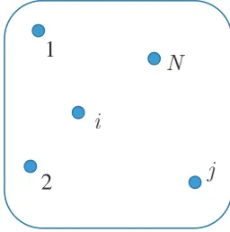
In an isolated N-body charged particle system, as shown in Fig. 1, the non-relativistic equation of motion for thei-th particle with an electric chargeqiand a massmiis
mi dui
dt=qi
N
ji
qj 4π0
ri−rj |ri−rj|3
. (1)
whereriandui stand for the position and the velocity of thei-th particle. Hereafter, the calculation using the above equation of motion, Eq. (1), will be referred to as the direct integration method (DIM).
WhenN≥3, it is well known that no exact/analytical solution can be obtained, and one should be content with solutions approximated by using a numerical integration method. In principle, to arbitrary error levels, the numeri-cal solution can be found. However, it is practinumeri-cally impos-sible for the large number of particles, i.e. N ≫ 1, since the number of force calculations on the right-hand side of Eq. (1) is in proportion to N2. Moreover, the number of
time steps tends to increase with increasingN, so the total CPU time should scale asN3.
The efficient, fast algorithms to calculate inter-particle forces include the tree method [1, 2], the fast multipole expansion method (FMM), and the particle-mesh Ewalt (PPPM) method [3]. Efforts have been made to use paral-lel computers and/or to develop special-purpose hardware to calculate interparticle forces, e.g., the GRAvity PipE (GRAPE) project [4]. The authors have recently devel-oped an algebraic model for multibody problems [5] and have shown that the momentum transfer cross-section with our model is in good agreement with the exact one [5, 6]. Unfortunately, this model turns out to lack sufficient accu-racy in predicting individual particle motions [6].
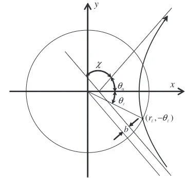
As shown in Fig. 2, which depicts the relative mo-tion of the particle pairi and jin the center-of-mass
co-author’s e-mail: [email protected]
Fig. 1 AnN-body system.
ordinate system, the scattering angle, χ ≡ π−2θ0, is
found byb = b0tanθ0, whereb is the impact parameter,
b0 ≡ e2/4πε0μg20 corresponds toχ = π/2 scattering, and
g0 is the initial relative speed atr = ∞andtheta = −θ0.
Hereμ ≡mimj/(mi+mj) is the reduced mass. In the bi-nary system with an impact parameterb, a typical velocity changeΔgin the relative velocity is given by
Δg=2g0sin
χ
2 ∼g0, ≡
b0
Δ. (2)
whereΔis the average interparticle separation.
In N-body systems with 1, such as the fusion plasmas, Eq. (2) suggests that three-or-more-body interac-tion is of the order of2 and can be ignored. Note that
the Debye lengthλDin fusion plasmas generally satisfies
λD Δ, thus, typical binary interaction is characterized
by the nondimensional parameter. This parameter is of the order ofU/K, whereU andKstand for the potential and kinetic energies, respectively.
In this study, we will propose the binary interaction approximation (BIA) to theN-body systems with 1, and compare it with the DIM, both using the six-stage fifth order Runge-Kutta-Fehlberg (RKF65) integrator [7,8] with
c
Fig. 2 Unperturbed relative trajectoryr = r(θ) in an orbital plane. The scattering center is at the origin. Impact pa-rameter isb=b0tanθ0.
an absolute numerical error tolerance of 10−16.
2. BIA: Binary interaction
approxim-ation to
N
-body problems
The equation of relative motion for the particle pair (i,j) in anN-body system used by the BIA is
μi jdgi j dt =
qiqj 4π0
ri j
r3
i j
. (3)
whereri j = ri−rj stands for the relative position,gi j = ui−uj is the relative velocity, andμi j = mimj/
mi+mj
is the reduced mass. In the BIA, the above equation is integrated, completely ignoring the other particles, from
t=0 tot= Δtto yieldΔri j andΔgi j. The total number of integrations isNC2=N(N−1)/2 for anN-body problem.
The individual changes in positionΔri, and velocityΔui, of thei-th particle are
miΔri=miuiΔt+ N
ji
μi jΔri j−gi jΔt
. (4)
miΔui= N
ji
μi jΔgi j. (5)
fori =1,2,· · ·,N. Note that the term within the paren-theses,δri j ≡Δri j−gi jΔtas shown in Fig. 3, on the right-hand side of Eq. (4) vanishes when the interaction between pair (i,j) vanishes. In other words, the BIA scheme is ex-act for free particles. Note also that the total momentum
P ≡ N
i=1miui is kept constant with this approximation,
since, from Eq. (4) andμi j=μji, N
i=1
miΔui= N−1
i=1
N
j=i+1
μi j
Δgi j+ Δgji=0. (6)
Fig. 3 Relative motion for particle pair (i,j). Scattering center is at the origin. The change in position of the particle with a massμi jisΔri j. If no interaction occurs, the change in
position isgi jΔtduring a time interval ofΔt.
which also guarantees the center of mass positionRCM to
be exact,
RCM(Δt)=RCM(0)+GCM(0)Δt, (7)
whereGCMis the center of mass velocity.
3. Calculation
3.1
Initial condition for an
N
=
122-body
pr-oblem
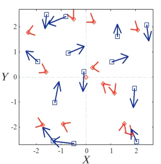
Figure 4 depicts the initial condition for a two-dimensionalN =122-problem, in which there are 61 pro-tons and 61 electrons. Note that only 26 particles near the origin are depicted in the figure. In this and the fol-lowing figures, positions are normalized by the interpar-ticle separationΔ ≡ n−1/3 and velocities by the relative thermal speed among electrons, geeth = √2veth. Squares with arrows in blue in Fig. 4 represent electron positions and velocities, and diamonds with arrows in red repre-sent protons. Spatial distribution is uniform with an av-erage particle distance beingΔ =n−1/3, and the velocity distribution is Maxwellian for both species with tempera-tures ofT = Telectron = Tproton = 10 keV. A number
den-sityn =1020m−3 is assumed, which yields the parameter
=1.67×10−71.
Since we have assumed Maxwellian velocity distribu-tions, no particle has a velocity of exactly zero, i.e., no particle at rest. In terms of numerical errors, however, we have found that the BIA method has given larger nu-merical errors, especially in position, for particles at rest than for those in motion. For this reason, we have inten-tionally assigned zero velocity to one proton at the origin (X,Y)=(0,0), as shown in Fig. 4. The trajectories of this proton as well as a typical electron will be shown in the next section.
3.2
Trajectories of a proton and an electron
Fig. 4 Initial positions normalized by the interparticle separa-tionΔ ≡ n−1/3 of an N = 122-body problem. Only 26 particles near the origin are depicted. Squares with arrows in blue represent the electron positions and veloc-ities, and diamonds with arrows in red represent protons. Spatial distribution is uniform for both protons and elec-trons. The Maxwellian velocity distribution is adopted for a given temperatureT=Telectron=Tproton.
Fig. 5 Motion of a proton initially at rest in the configuration space (left), and in the velocity space (right) for the N =122-body system. Symbols represent the initial and final position calculated with the BIA. The particle starts at the diamonds and moves along lines which are calcu-lated with the fullN-body integration, i.e., the DIM.
the average interparticle separationΔ≡n−1/3. Figures 5
and 6 show the trajectories in the configuration space (X,Y) on the left and velocity space (U,V) on the right for a pro-ton initially at rest and a moving electron, respectively. In both figures, the diamonds labeled ‘initial’ are initial points att = 0. The lines are trajectories obtained by using the DIM. Triangles indicate the final points att= Δtwith the BIA. The agreement between the BIA and the DIM is ex-cellent.
As shown on the right in Fig. 6, the complicated change in velocity with time, or the acceleration, is typ-ically reproduced well with the BIA, in which three-or-more-body interactions are ignored.
Fig. 6 Motion of an electron for theN=122-body system. Leg-ends are the same as in Fig. 5.
Table 1 Effective digits for calculated invariants of motion and CPU time forN =122. PX andPY are the total linear
momenta,LZis the total angular momentum,Eis the total
energy of the system.
method PX PY LZ E CPU time
DIM 16 15 16 16 3.4
BIA 16 15 15 12 0.2
unit digit sec
3.3
Errors and e
ff
ective digits of invariants
There are four invariants of motion in an isolated two-dimensional system: the total linear momenta P = (PX,PY), the total angular momentumLZ, and the total en-ergyE. Effective digits for the calculated invariants of mo-tion and the CPU time forN=122 are listed in Table 1. In the table withri=(Xi,Yi), andui=(Ui,Vi),PX = N
i=1
miUi. (8)
PY= N
i=1
miVi. (9)
are the total linear momenta,
LZ= N
i=1
mi(XiVi−YiUi). (10)
is the total angular momentum, and
E=1
2 N
i=1
miu2i + 1 4π0
N−1
i=1
qi N
j=i+1
qj |ri−rj|
. (11)
is the total energy of the system.
initial conditions forN=122-body problem. The conser-vation inLZ, however, is generally close to that of E for different initial conditions and the numbers of particlesN. As for the CPU time, the BIA is 17 times faster than the conventional DIM for N = 122. Since the speed-up ratio depends essentially on the number of particlesN, cal-culations for differentNwill be examined in the following subsection.
3.4
CPU time dependence on
N
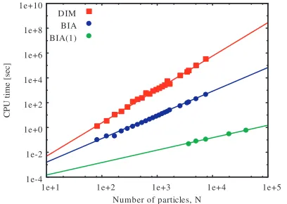
We made a calculation similar to the foregoing section while varying the number of particlesN. The CPU time dependence on N is depicted with fitting lines in Fig. 7, in which CPU time inversions are found for the DIM, i.e., longer CPU timeτCPU
DIM(N)> τ CPU
DIM(N) for fewer particles
N<Nat aroundN ∼700 and 1600. Such inversions can occur because the integrator used here, RKF65, controls the time-step size during the calculation according to the given error tolerance. The CPU time for the DIM scales as
τCPU
DIM∼1.2×10−
5×N2.7sec.
(12) and that for the BIA as
τCPU
BIA ∼3.4×10−
5×N1.9sec.
(13) both using the RKF65 with the same absolute error toler-ance of 10−16. Also, BIA(1) is the CPU time to calculate only one particle, which scales as
τCPU
BIA(1)∼1.1×10−
5×N1.0sec.
(14) If we are interested in the motion of only one test particle-iat a timet = Δtfrom initial conditions att =0, it is possible with the BIA to calculateri(Δt) andui(Δt)
completely in parallel, since it is based on the principle of superposition ofΔri j andΔui j using Eqs. (4) and (5). For example, for an 108-body problem, which corresponds to full three-dimensional Coulomb interactions in a fusion plasma within the Debye sphere, the DIM would need a CPU time of 3×10⁸years, while the BIA would require
less than an hour to calculate a test particle motion. As was shown on the right in Fig. 6, the temporal elec-tron acceleration is complicated due to its small mass. For a given numerical error tolerance, this tends to make the common time-step smaller and consequently make the to-tal CPU timeτCPU longer especially in the DIM. On the
other hand, the BIA with the same error tolerance as the DIM is apair wise variable time-step scheme, since the time step for the pair (i,j) is independent of that for any other pairs (i,j).
4. Summary and Discussion
The binary interaction approximation (BIA) to N -body problems is proposed. The BIA conserves total linear momenta in principle, and is apair wisevariable time-step scheme when used with an integrator using the embedded
Fig. 7 CPU timeτCPU dependence on the number of particles Non a typical PC. Red squares represent the CPU time for the DIM with a fitting line in red,τCPU
DIM∝N
2.7. Blue
circles represent the CPU time for the BIA with a fitting line in blue,τCPU
BIA ∝N
1.9. Also, BIA(1) is the CPU time to
calculate only one particle, which scale asτCPU
BIA(1)∝N
1.0.
formula, such as the Runge-Kutta-Fehlberg scheme [7, 8]. Other invariants, such as the total angular momentum and total energy, are conserved to at least 12 effective digits for a two-dimensional hydrogen plasma ofT = 10 keV and
n=1020m−3, in which∼1.67×10⁻⁷. The CPU time of
the BIA scales asτCPU BIA ∝N
1.9for such a plasma. Note that
with the BIA, it is possible to calculate only one particle’s motion [6] with the CPU time proportional toN.
The numerical results presented here are for two-dimensional systems with low density and high tempera-ture, i.e., 1, which is the most appropriate for the BIA. We will soon apply the BIA to three-dimensional cases and/or to systems with∼1, such as gravitational
N-body systems, in the near future.
Acknowledgement
The author thanks Dr. A. Wakasa, Prof. Y. Matsumoto, and Prof. M. Itagaki for fruitful discussions on the subject. The author also acknowledges the continuous encourage-ment of the late Prof. T. Yamashina. This research was par-tially supported by a Grant-in-Aid for Scientific Research (C), 21560061.
[1] A.W. Appel, An Efficient Program for Many-Body Simula-tion, SIAM J. Sci. Stat. Comput.6, 85 (1985).
[2] J.E. Barnes and P. Hutt, A hierarchical O(NlogN) force-calculation algorithm, Nature324, 446 (1986).
[3] P.P. Brieu, F.J. Summers and J.P. Ostriker, Cosmological Simulations Using Special Purpose Computers: Implement-ing P3M on GRAPE, APJ453, 566 (1995).
[4] J. Makino, M. Taiji, T. Ebisuzaki, and D. Sugimoto, GRAPE-4: A Massively Parallel Special-Purpose Computer for Collisional N-Body Simulations, APJ480, 432 (1997). [5] S. Oikawa and H. Funasaka, Algebraic analysis approach for
of velocity changes, ITC-18, P2-58(2008); also submitted to PFR.
[7] E. Fehlberg, Low-order classical Runge-Kutta formulas with step size control and their application to some heat transfer problems, NASA Technical Report 315 (1969).