A Comparative Study of Uncertainty Estimation Methods in Deep Learning Based Classification Models

(1)

A Comparative Study of Uncertainty

Estimation Methods in Deep Learning

Based ClassiĄcation Models

Iswariya Manivannan

Publisher: Dean Prof. Dr. Wolfgang Heiden

Hochschule Bonn-Rhein-Sieg Ű University of Applied Sciences, Department of Computer Science

Sankt Augustin, Germany

September 2020

(2)

Bosch Center for

ArtiĄcial Intelligence (BCAI)

This work was supervised by Laura Beggel Deebul Nair Paul G. Plöger

Copyright c÷ 2020, by the author(s). All rights reserved. Permission to make digital or hard copies of all or part of this work for personal or classroom use is granted without fee provided that copies are not made or distributed for proĄt or commercial advantage and that copies bear this notice and the full citation on the Ąrst page. To copy otherwise, to republish, to post on servers or to redistribute to lists, requires prior speciĄc permission.

Das Urheberrecht des Autors bzw. der Autoren ist unveräußerlich. Das Werk einschließlich aller seiner Teile ist urheberrechtlich geschützt. Das Werk kann innerhalb der engen Grenzen des Urheberrechtsgesetzes (UrhG), German copyright law, genutzt werden. Jede weitergehende Nutzung regelt obiger englischsprachiger Copyright-Vermerk. Die Nutzung des Werkes außerhalb des UrhG und des obigen Copyright-Vermerks ist unzulässig und strafbar.

(3)

Abstract

Deep learning models produce overconfident predictions even for misclassified data. This work aims to improve the safety guarantees of software-intensive systems that use deep learning based classification models for decision making by perform-ing comparative evaluation of different uncertainty estimation methods to identify possible misclassifications.

In this work, uncertainty estimation methods applicable to deep learning models are reviewed and those which can be seamlessly integrated to existing deployed deep learning architectures are selected for evaluation. The different uncertainty estimation methods, deep ensembles, test-time data augmentation and Monte Carlo dropout with its variants, are empirically evaluated on two standard datasets (CIFAR-10 and CIFAR-(CIFAR-100) and two custom classification datasets (optical inspection and RoboCup@Work dataset). A relative ranking between the methods is provided by evaluating the deep learning classifiers on various aspects such as uncertainty quality, classifier performance and calibration. Standard metrics like entropy, cross-entropy, mutual information, and variance, combined with a rank histogram based method to identify uncertain predictions by thresholding on these metrics, are used to evaluate uncertainty quality.

The results indicate that Monte Carlo dropout combined with test-time data augmentation outperforms all other methods by identifying more than 95% of the misclassifications and representing uncertainty in the highest number of samples in the test set. It also yields a better classifier performance and calibration in terms of higher accuracy and lower Expected Calibration Error (ECE), respectively. A python based uncertainty estimation library for training and real-time uncertainty estimation of deep learning based classification models is also developed.

(4)

(5)

Acknowledgements

I would like to thank my supervisors Prof. Dr. Paul Pl¨oger, Deebul Nair and Laura Beggel from Bosch Center for Artificial Intelligence (BCAI) for providing the opportunity to work on this Research and Development project.

I would like to thank Laura Beggel and Deebul Nair for their continuous en-couragement, guidance and support throughout this project. I would also like to thank William Beluch and other BCAI colleagues for their inputs and BCAI for this wonderful opportunity.

Finally, I extend my gratitude to my friends, especially Sathiya Ramesh and my family for their endless support, motivation and love.

(6)

(7)

1 Introduction

The effectiveness of deep learning based image classification models over other traditional machine learning methods is undeniable. Despite their high accuracy, often an unrealistic high confidence value is attributed to wrong predictions [14], [34]. As a result it is important for users to be aware of the ramifications of the decisions made by the deep learning model in order to mitigate the adverse socio-economic impacts of unreliable predictions from models. One solution to address the problem of unreliable predictions is to produce a reliability score along with the model predictions. The uncertainty estimate also called the negative reliability score (i.e., the higher the uncertainty, the lesser is the reliability), helps the user understand what the classifier knows and what it does not know. This enables deep learning practitioners to make informed decisions in cases of high uncertainty, such as ignoring the model’s predictions and later re-training the model with those highly uncertain inputs to improve performance and so on. In this work we explore the power of uncertainty estimation to circumvent ”the problem of accidents in machine learning” [2] to a certain extent, where the unintended errors produced by the model can have potentially harmful consequences.

1.1 Motivation

Deep learning models do not provide reliable predictions. Their increasing usage in various domains such as medical diagnosis [37], autonomous driving [35], or drug discovery [44] can be attributed to the fact that they are able to quickly

(10)

analyze and make predictions on large diverse datasets with high accuracy. However, incorrect model predictions in safety-critical applications endanger human lives. One such example is when IBM’s Watson supercomputer often gave erroneous, unsafe treatment recommendations to patients [48]. Another instance is the accident caused by Uber’s self-driving car resulting in the death of a pedestrian, due to the fact that its perception model failed to detect the person on a bicycle most likely because of insufficient illumination [42]. In most of the cases, the exact reason remains unknown because deep learning models often act as a black-box [46]. Although several approaches try to uncover the actual operating mechanism under the hood, explainable AI is far from maturity [1]. As a result, we wish to take an alternate route by making the model speak for itself by providing uncertainty estimates when it is unsure of its predictions, as in the case of the above mentioned examples.

One of our applications of deep learning involves the use of a deep neural network based classification model for optical inspection at Robert Bosch GmbH. The main objective of the optical inspection process is to distinguish defective parts from non-defective ones. The non-defective parts are produced when the manufacturing process is improper/incomplete and are generally manually classified by a human inspecting the images of these parts. The optical inspection process is automated by deploying a trained deep learning based classification model that can distinguish between the defective and non-defective parts. It is necessary that the automation of this inspection process by means of a deep learning model guarantees that defective products are not being classified as non-defective ones (i.e., a low miss-rate). Hence to ensure that defective parts do not get classified as non-defective ones, uncertainty estimation techniques are applied to provide a statistics on how reliable the model’s predictions are.

Another similar application uses a deep neural network based perception mod-ule in the KUKA YouBot, an industrial service robot extensively used in the RoboCup@Work league [31]. Robots participating in the competitions of the RoboCup@Work league are required to execute efficient and intelligent solutions to the given scenarios, such as pickup and delivery of tools from different stations. The perception module uses a deep learning model is to extract and classify the objects present in the station image from the robot’s camera. Once an object is classified as a tool, it is picked up by the robot’s arm, placed on the robot’s base and carried

(11)

Chapter 1. Introduction

(a) YouBot picking up a carrot (b) YouBot picking up a beer can

Figure 1.1: Images of KUKA YouBot picking up objects which are not tools from the station [38].

to the delivery station. Fig. 1.1 shows the YouBot accidently picking up a carrot and a beer can because of confident misclassifications made by the deep learning based classification model. As a result, the robot receives a penalty for picking up a non-tool object. However, if the model is able to provide an uncertainty score along with its predictions (thereby indicating that it is unsure of its predictions), then alternative solutions can be devised, such as ignoring current object and moving on to the next.

1.2 Challenges and Difficulties

Uncertainty estimation methods need to address the following problems to yield reliable confidence estimates.

• Deep learning models produce point estimates as outputs, which do not yield any measure of uncertainty. Therefore, it is imperative that models must be adapted to produce distributional outputs from which uncertainty estimates can be extracted.

• The softmax function used in deep learning based classification models produce overconfident point estimates. The softmax activation is used in the last layer of the network to scale each of the logit values per class to a value between 0 and 1. The softmax outputs of all logits sum to 1, thereby giving the softmax an interpretation that it converts the predicted logit values into class confidence probabilities. The model’s prediction is given by the class to which

(12)

the maximum confidence value is attributed. However, the softmax is known to produce very high confidence values even when the model is given a input data which it has not seen during training [14].

• Deep learning models do not provide calibrated outputs [22]. Calibration measures the reliability of the model in producing consistent predictions. A consistent prediction for instance would refer to the case where the classifier is 90% accurate when it makes a prediction with 90% confidence. For a calibrated model, the predicted confidence estimates should reflect the probability of the prediction being correct, i.e., the predicted confidence and model accuracy should bear a linear relationship. This does not hold for deep learning models, as calibration is not taken into account during the training process.

• An important constraint posed by our optical inspection problem is that uncertainty estimation methods should be fast and packageable as an auxiliary module which can be integrated on top of existing deep learning models. This is because we aim to estimate the predictive uncertainty of an already deployed model. Thus, these methods should not introduce major architecture changes that would cause the re-training and hyper-parameter tuning of the deployed deep learning model.

1.3 Problem Statement

The purpose of uncertainty estimation is to obtain reliable predictions from a classifier. The single point estimates predicted by existing deep learning classifiers need to be replaced by predictive distributions to quantify uncertainty (Fig. 1.2). It is vital for the predictive distributions to be sharp for highly certain predictions and flat for data-points where the classifier is not confident about its predictions. The sharper the individual predictive distributions are, the lesser is the uncertainty per data-point and vice-versa. Therefore, we first identify uncertainty estimation methods that satisfy the constraint posed by our optical inspection problem (section 1.2) and are able to obtain predictive distributions from which uncertainty estimates can be extracted.

In the case of deep learning models, sharpness is usually achieved during the training process by minimizing the Negative Log-Likelihood (NLL) objective. The

(13)

Chapter 1. Introduction

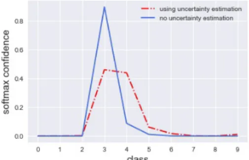
(a) Deer image (class 4) from CIFAR10 dataset

(b) Distribution of softmax confidence probabilities per class

Figure 1.2: Fig. 1.2a shows the image of a deer belonging to class 4 of the CIFAR-10 dataset classified using a VGG-16 model. The blue line depicts the over-confident wrong prediction made by the model when it is not using any uncertainty estimation method. The model makes a prediction that the image is a cat (class 3) with a high confidence probability of 0.89. Fig. 1.2b illustrates the reduction in sharpness of the softmax confidence when using uncertainty estimation methods (Monte Carlo dropos ut and test time augmentation).

result of this training process yields deep learning models which produce overconfident predictions (popularly referred to as the softmax overconfidence problem [14]). As a result, it is desirable to have flatter distributions (i.e., with greater uncertainty) to compensate for the unreliable over-confident predictions. Hence, we compare uncertainty estimation techniques applicable to deep learning models, which are not only able to produce predictive distributions but also reduce their excessive sharpness, leading to an increase in uncertainty. Appropriate metric(s) that are able to quantify the increase in model uncertainty on the application of different methods have to be selected from the vast collection available in the literature. The selected metric is used to measure the uncertainty of the misclassified samples in the dataset and also to identify the method which detects the highest number of the misclassified samples as uncertain.

While it is important to reduce the excessive sharpness of the predictions, it is also necessary to consider the notion of classifier calibration (more details in Chap. 3), which gives the statistical consistency between the model’s predictions and the observations [20]. In practice, deep learning models have the inherent property

(14)

of being miscalibrated [22] and the improvement in classifier calibration after the application of different uncertainty estimation methods will be investigated. This is essential because sharpness or calibration by themselves alone cannot guarantee reliable predictions and hence, it is necessary to jointly optimize for both. As a result it is beneficial to have uncertainty estimation methods that are able to tackle both the softmax over-confidence and the calibration problem.

(15)

2 Background

This chapter presents an overview of the various techniques used to formalize an uncertainty estimation procedure applicable to models ranging from simple Bayesian models to neural networks (for more details refer Chap. 2 and 3 of Gal [13]). Although, these methods are fundamental and do not scale well to deep neural networks, they form the basis of many uncertainty estimation methods developed for deep neural networks discussed in the upcoming chapters. These techniques aim at obtaining output probability distributions, which are in general able to capture the statistical dispersion of the represented quantity -a necessary attribute for quantifying uncertainty- from the model at hand.

2.1 Bayesian Modeling

The Bayesian approach is used to quantify the uncertainty in our beliefs using probability distributions [40]. Let us consider the low dimensional input data-points given by X = x1, x2, ..., xn and their corresponding output labels Y =y1, y2, ..., yn generated from some unknown probability distribution. We are required to find a function which is a mapping between the input data-points X and the outputs Y. Suppose we use a Bayesian model parameterized by the model parameters ω which are drawn from the initial prior distribution P(ω) to learn this mapping function, then the prior signifies our initial belief on this mapping function. The goal of the learning process is to modify the prior distribution based on the training data in such a way that the model is transformed into an ideal or close to ideal mapping

(16)

function between X and Y. The below equation depicts how the prior distribution of the weights P(ω) is modified to give the posterior P(ω|X, Y) based on the data likelihood P(Y|X, ω). P(ˆω|X, Y) = P(Y|X, ω)P(ω) P(Y|X) (2.1) where, P(Y|X) = Z P(Y|X, ω)P(ω)dω (2.2) The denominator in Eq. (2.1), which is central to the computation of the posterior distribution is called the model evidence. Since Eq. (2.2) performs a marginalization by computing the integral over all possible values ofω, it is also called the marginal likelihood. The use of conjugate priors facilitates the easy computation of the posterior in Eq. (2.1). This is because conjugate priors mimick the form of the likelihood distribution and yield a posterior which is in the same family as the prior.

Having computed the posterior of the weights P(ˆω|X, Y), the next step in a Bayesian model would be to make an inference for a new test data-point. This essentially means that the model is expected to make a predictiony∗ for a test input

x∗ _{given its learned weights ˆ}_ω_{. Given the test input, the output can be inferred by}

integrating over all values of the posterior probability distribution of ˆω.

P(y∗|x∗, x, y) =

Z

P(y∗|x∗,ωˆ)P(ˆω|X, Y) (2.3)

From Eq. (2.2) and (2.3), it is seen that a simple Bayesian model is capable of providing a distributional output (weights and predictions), in contrast to a single point estimate which is generally being used/obtained from classical non-Bayesian neural networks. Distributions are very convenient because uncertainty estimates can be effortlessly extracted (for instance computing the variance) and point estimates are obtained using various statistics such as mean, median or mode. However, it is not possible to obtain such predictive posterior distributions in deep neural networks using such simple Bayesian modeling tools. This is because the computation of the posterior in Eq. (2.1) and the closed form computation of the integral in Eq. (2.3) is intractable due to the complex data likelihood function and the presence of millions of weight parameters with infinite combinations of values. As a result, we resort to

(17)

Chapter 2. Background

approximate inference techniques, when closed form computation is not possible.

2.2 Variational Inference

When it is not possible to analytically compute the true posterior P(ω|X, Y), variational inference [8] is used. It involves using an approximate variational dis-tribution q(ω) parameterized by θ instead of the true posterior P(ω|X, Y). The parameter θ is also called a latent variable θ, since it is not directly observed but inferred from the observed data-points X. It is estimated using an optimization procedure. The aim of the optimization process is to find the set of latent variables

θ which can best describe the observed data. The Kullback-Leibler (KL) divergence (also called relative entropy) [33] which is used to measure the similarity between the two distributions is used as the optimization objective. Thus, the optimization process aims to minimize the KL divergence so thatq(ω) is very close to P(ω|X, Y). The below equation gives the KL divergence between the two distributions

KL(q(ω)||(P(ω|X, Y)) = Z q(ω)log( q(ω) P(ω|X, Y))dω = Z q(ω)log(q(ω))dω− Z q(ω)log(P(ω|X, Y))dω = Z q(ω)log(q(ω))dω− Z q(ω)log(P(ω, X, Y))dω+log(P(X, Y)) (2.4) where, ELBO=− Z q(ω)log(q(ω))dω+ Z q(ω)log(P(ω, X, Y))dω ≤log(P(X, Y)) (2.5) The ELBO as the name suggests is a lower bound on the probability of observed data (also called evidence). Substituting Eq. (2.5) in Eq. (2.4) gives the following equation.

KL(q(ω)||(P(ω|X, Y)) = −ELBO+log(P(X, Y)) (2.6) Eq. (2.6) shows that an alternative to minimizing the KL divergence objective is to maximize the ELBO. The log probability log(P(X, Y)) of the data is an additive constant which can be ignored during the optimization process. Essentially this

(18)

means that increasing the lower bound on the data makes it closer to the true posterior P(ω|X, Y) distribution. This process of using an approximate distribution

q(ω) to model the true posteriorP(ω|X, Y) and optimizing the parameters ofq(ω) by minimizing the KL divergence is called variational inference. Variational inference has two major advantages: Firstly, the marginalization process Eq. (2.2) required to compute the true posterior P(ω|X, Y) is not necessary. Secondly, it outputs a probability of weights q(ω) from which uncertainty estimates can be derived, in contrast to deep learning methods which provide point-estimates of the network weights. However, this also does not scale well to large datasets or deep learning models with several parameters because computing the integral in Eq. (2.4) is intractable. We shall discuss several methods in Chap. 3 that apply an approximate Bayesian inference procedure to deep neural networks to obtain output probability distributions instead of point estimates.

2.2.1 Approximate inference

Approximate inference in neural networks can be traced back to Hinton and Van Camp [26] who utilize the Minimum Description Length (MDL) principle [47] to restrict the amount of information on the weights by adding noise to reduce over-fitting. Here a neural network with a single hidden layer is trained with its weights drawn from an independent Gaussian distribution. During back-propagation the gradients for the mean and variance of the respective Gaussian distributions can be computed because it is possible to perform analytical integration over the Gaussian distribution. This technique is applicable only for single layer neural networks because of its computational complexity, and it relies on the simplifying assumption that the weights of the hidden layer are drawn from independent Gaussian distributions. Barber and Bishop [6] improved on the work of Hinton and Van Camp [26] by modeling the dependency between the weights using non-diagonal covariance matrices. However, this comes at an additional increased computational cost and it is impossible to perform this analytical computation when this method is applied to deep neural networks.

Graves [21] extends the work of Hinton and Van Camp [26] to a recurrent neural network by using Monte Carlo sampling for computing the posterior of the weights.

(19)

Chapter 2. Background

But Monte Carlo estimators are known for their high variance noisy estimates and when combined with Stochastic Gradient Descent (SGD) optimizer, perform poorly in terms of noisy, inaccurate results. Blundell et al. [9] uses the re-parametrization trick, which was developed by Kingma and Welling [30] in the context of latent variable models, to obtain uncertainty estimates of the weights of the neural network. The re-parametrization trick allows a continuous random weight parameter of a neural network drawn from a Gaussian distribution to be expressed as a sum of a deterministic variable and a noise parameter sampled from a Gaussian distribution. Applying this re-parametrization trick to the previous methods, where the weights are directly sampled from independent Gaussian distributions, enables the representation of each weight parameter by a deterministic mean µ and standard deviation σ

parameter, with a small Gaussian noise added to σ. During back-propagation the deterministic gradients are computed with respect to µand σ for each weight parameter. This method is more efficient as compared to the previous methods of representing the weights as a distribution. However, the number of parameters of the network are doubled since each weight is represented by its mean and standard deviation, hence training and inference would cost more in terms of time and memory.

(20)

(21)

3 Related Work

In the previous chapter, we have discussed several techniques to obtain output distributions from a neural network. However, most of these techniques are either analytically intractable or are slow, approximate and inaccurate due to the complexity of deep neural networks. This chapter presents the state-of-the-art uncertainty estimation methods which can be applied to deep neural networks. The uncertainty estimation methods can be broadly classified into two categories - Bayesian and non-Bayesian. These methods extend the techniques discussed previously to obtain approximate output distributions with fast and accurate uncertainty estimates.

The obtained predictive uncertainty is of two types epistemic uncertainty and aleatoric uncertainty [57], or a combination of both. Epistemic uncertainty refers to the uncertainty in model parameters, especially when the model has not seen enough data. This type of uncertainty is reducible as it decreases when more data is given to the model. Aleatoric uncertainty on the other hand, refers to noise in the data (image noise in the case of image datasets). This is further classified into two types - homoscedastic and heteroscedastic noise. The former denotes the noise that is prevalent in the entire dataset, while the latter represents the noise that is unique to each data-point.

(22)

3.1 Approximate Bayesian Methods for Uncertainty

Estimation

The training of Bayesian models usually involves placing a prior distribution over the parameters of the model, computing the posterior given the data likelihood and performing inference over the test data by marginalizing over the posterior of the learned parameters (Section 2.1). Bayesian modeling and inference are intractable for deep learning models due to the reasons discussed in the previous chapter. For this reason we resort to approximation methods for posterior computation and marginalization. our problem statement requires a deep learning based classification model which has practical time and resource constraints, and should also be able to handle high dimensional inputs such as images. Hence, we are seeking uncertainty estimation methods that are applicable to current deep learning architectures such as VGG [53], ResNet [24], Xception [10], MobileNet [27]. On the other hand, Bayesian uncertainty estimation methods developed in the context of Bayesian Neural Networks (BNN) developed by Depeweg et al. [11], Hern´andez-Lobato and Adams [25], Blundell et al. [9] are not discussed here. This is because it is not possible to deploy BNNs for real-world scenarios because training and inference is very slow.

3.1.1 Monte Carlo dropout

Dropout is a regularization technique used in deep learning models to reduce over-fitting [54]. Dropout is originally designed to be used during the training phase where the model is trained by randomly turning off or dropping a set of neurons with a certain probability, called the dropout probability (or dropout mask). This in turn gives a regularization effect because it indirectly combines many different network architectures approximately and efficiently. During test time, dropout is deactivated and predictions are made without dropping any weights.

A neural network with dropout applied to its weight layers can be cast an approximate Gaussian Process (GP) [41]. It is a well known fact that making an inference from a GP is advantageous since the output is a distribution rather than a point estimate and uncertainty estimates can be drawn from this output distribution. Therefore, by approximating a deep neural network to a GP one can obtain uncertainty estimates for the predictions made by the network [14].

(23)

Chapter 3. Related Work

The below equation 3.1 describes a typical loss function used in deep neural networks where, the first term on the right hand side represents the squared loss or the softmax loss between the network predictions ˆyi and the target yi for N training samples, and the second term is theL2 regularization used to reduce over-fitting. L2

regularization contains the product of the weight decay constant λ and the squared

L2 norm of the weightsWi and biases bi of the L-layered network.

Ldropout = 1 N N X i=1 E(yi,yˆi) +λ L X i=1 (||Wi||22+||bi||22) (3.1)

The predictive probability for a test data-point (x∗_{, y}∗_{) of the deep GP model with}

weights ω trained on the training data (X, Y) is given as follows,

P(y∗|x∗, X, Y) =

Z

P(y∗|x∗, ω)P(ω|X, Y)dω (3.2)

The computation of the true posterior of the weights P(ω|X, Y) is intractable, hence an approximate posterior given by the dropout weights q(ω) is used. This approximate inference problem is solved by minimizing the KL divergence objective.

−

Z

q(ω)log(p(Y|X, ω))dω+KL(q(ω)||p(ω))dω (3.3)

The minimization objective in Eq. (3.3) is solved by approximating the integral with a Monte Carlo substituting a regularization term with prior-length scale l and model precision τ as shown below.

LGP−M C ∝ 1 N N X i=1 −log(p(yn|xn,ωˆn)) τ + L X i=1 ( pil 2 2τ N||Mi|| 2 2+ l2 2τ N||mi|| 2 2) (3.4)

It can be seen that Eq. (3.1) is similar to Eq. (3.4) and proves that the minimization of the loss function in a dropout neural network is equivalent to minimizing the KL divergence between the approximate posterior obtained using the dropout weights and the true posterior of the deep GP. During inference the approximate predictive distribution q(y∗_|_x∗_{) is obtained using the approximate posterior} _q₍_ω_{) (weights of}

(24)

the dropout network).

q(y∗|x∗) =

Z

P(y∗|x∗, ω)q(ω)dω (3.5) The integral can be approximated using Monte Carlo estimation, which essentially means that the average of the prediction confidences over T forward passes is taken, where W_lt is the dropout weight for layer l and forward pass t.

Eq(y∗_|_x∗₎(y∗) = 1 T T X t=1 ˆ y∗(x∗, W₁t, ..., W_Lt) (3.6)

The expected prediction confidence Eq(y∗_|_x∗₎(y∗) for a test data-pointx∗ with label

y∗ is obtained by computing the average of the predictionsy∗ from T forward passes. The expected prediction confidence is a more reliable estimate of the model prediction confidence on a particular data-point as compared to the prediction from a single forward pass. Uncertainty estimates can be obtained by computing the variance or entropy of the predictions over several forward passes. The number of forward passes depends mostly on the model and dataset at hand but an approximate upper limit on the number of forward passes is 50.

The approach discussed so far yields uncertainty estimates which are a function of the model weights, more specifically the weights produced by dropout. Hence, it is more appropriate to classify the uncertainty estimates from Monte Carlo (MC) Dropout as epistemic uncertainty estimates. Kendall and Gal [29] introduces a slight modification to the network architecture and loss function of the deep learning model so as to produce an additional estimate of aleatoric uncertainty, which is a measure of the inherent noise in the dataset. A typical classification model produces as many logit values per image fi as the number of classesc in its last layer, which is then passed to an activation function such as softmax to give per class confidence values. An additional logit is added to the last layer to provide an aleatoric uncertainty estimate per image. Thus, the network has two output nodes, one producing the softmax output sof tmax(fi) and the other producing an aleatoric uncertainty estimate σ. An extra term is added to the loss function of the network in order to optimize the

(25)

weights of σ as shown in Eq. (3.7).

Laleatoric = 1 N N X i=1 log 1 M M X m=1

exp( ˆfi,m,c−log

X c ˆ fi,m,c) (3.7) where, ˆ fi,m =fi+σiǫm, ǫm ∼ N(0,1) (3.8) The aleatoric component of the loss function models an approximation to the distribution of true noise per data-point by drawing samples from a Gaussian prior Eq. (3.8) and performing Monte Carlo integration of M such samples.

This method of aleatoric uncertainty estimation can be combined with MC dropout to obtain both the aleatoric and epistemic uncertainty estimates per data-point. The combined loss function is given in Eq. 3.9.

Lcombined= 1 N N X i=1 E(yi,yˆi) + 1 N N X i=1 log 1 M M X m=1

exp( ˆfi,m,c−log

X

c ˆ

fi,m,c) (3.9)

These methods suffer from minor drawbacks depending on the real-time applica-tion they are used for. The quality of epistemic uncertainty is directly proporapplica-tional to the the number of MC samples but an increase in number of MC samples per image results in an increased inference time. In situations where it is necessary to obtain quick uncertainty estimates, a compromise on uncertainty quality must be made by reducing the number of forward passes when choosing MC dropout. Aleatoric uncertainty estimation on the other hand has no such trade-off issues between inference time and quality but comes with its own cost, as it introduces changes to the network architecture and results in model re-training. This might not be useful for already deployed models, however MC dropout can be used here for obtaining uncertainty estimates given the existence of dropout layers in the deployed model.

3.1.2 Stochastic batch normalization

Input data fed in batches to a neural network is non-linearly transformed (using relu, tanh, sigmoid, leaky relu and others) as it passes from layer to layer until it

(26)

reaches the output layer. This non-linear transformation in each layer causes arbitary scaling of the data thereby causing a distributional change with respect to the original input data. Thus, the weights of each layer of the network are optimized with respect to the distribution of data from the previous layer and not with respect to the input distribution. This distributional change of the input data as it passes through the layers of the network is termed as covariate shift [52]. Batch normalization attempts to rectify this problem by normalizing the batch of data in each layer [28] before it is given to the non-linearity. The batch norm paramters per layer, which include the mean µB and the variance σB are computed. The normalization is done by shifting each data-point with the mean and scaling it with the variance in every dimension of the data. A small constantǫ is added to the variance to avoid division by zero errors.

µB = 1 m m X i=1 xi (3.10) σB = 1 m m X i=1 (xi−µB)2 (3.11) ˆ xi = xi−µB p σ2 B+ǫ (3.12) During test time the batch norm parameters, i.e. the mean and variance per layer, saved during the training phase are used.

Similar to MC dropout uncertainty estimates can be obtained using batch nor-malization by introducing stochasticity in the network during test time. However, unlike dropout the stochasticity is in the batch norm parameters and not in network weights. A valid mathematical formulation equivalent to MC dropout in Section 3.1.1 is also obtained by replacing the weights w with the batch norm parameters

µB and σB.

In order to obtain uncertainty estimates at test time, T different batch norm parameters are required for T forward passes. These batch norm parameters are obtained by passing T different batches of training data through the network. As a result, to compute the uncertainty for a single test data, T different batches of training data have to sampled and T forward passes of these sampled batches are required to get the batch norm parameters per batch [56]. It is computationally

(27)

expensive when this process has to be repeated for each data-point in the test set. Hence, an alternate option would be to store the batch norm parameters of T different training batches during training itself, and then later use them when required at test-time. This method performs at par with MC Dropout, however deteriorates when the batch size is less than 16, as batch norm itself proves to be ineffective in this case.

Another efficient method would be to construct an approximate distribution of the batch norm parameters µB, σB of each layer of the trained model. During test time for multiple forward passes any number of these parameters can be drawn by sampling from this distribution. Atanov et al. [4] suggests the use of a normal and a log normal distribution to approximate the meanµB and the varianceσB respectively. This choice of distributions is able to the fit real distributions of these parameters more closely and can be verified by the similarity between these distributions and the empirical distribution of µB, σB obtained from the training batches. Although, uncertainty estimates are obtained from the output predicted posterior, this method provides over-confident predictions as compared to MC dropout.

3.1.3 Test-time data augmentation

Data augmentation is a method used to increase the size of the training set when there are insufficient training samples. It involves applying spatial transformations such as rotation, flip, random crop, shear, brightness and contrast variations and so on to the training images. This allows the network to efficiently explore samples in the neighborhood of a particular training image. Uncertainty estimates can be obtained by applying data augmentation at test time. This would mean that several augmented versions of a single image is fed to the model for evaluation and the model prediction confidences for each augmented version is recorded. The entropy/variance of the predicted confidence values yields uncertainty estimates. Since the variations introduced are image specific, the uncertainty estimates more accurately describe the heteroscedastic aleatoric uncertainty [5], [59]. Mathematically, uncertainty estimation using test-time augmentation can be formulated using approximate Bayesian inference, similar to MC dropout [59]. The difference here is that the inference is performed over the parameters of the spatial transformation unlike MC

(28)

dropout where inference is over the network weights. Let us consider an input image

X0 to which the transformation operator T with parameters α is applied. The noise

in the transformation process (for example, due to down-sampling or approximation errors) is modeled as a Gaussian noise τ.

X =Tα(X0) +τ (3.13)

The transformed input image X is given to a classifierH(w, X) which is parame-terized by the weights w. Thus, the posterior over the transformation parameterα

and the noise parameter τ is given as follows.

P(α, τ|X0, Y) =

P(Y|X0, α, τ)P(α, τ)

P(Y|X0)

(3.14) Using the posterior, inference is made at test-time on a sample image x∗₀ and the prediction of the model is denoted by y∗.

P(y∗|x∗₀, X0, Y) =

Z

P(y∗|x∗₀, α, τ)P(α, τ|X0, Y)dατ (3.15)

This type of Bayesian inference is practically impossible, since neither the posterior (in Eq. 3.14) nor the integral in Eq. 3.15 can be computed. This is because there are innumerable transformations that can be applied to an image, thereby causing α to take on infinite values. For this reason, approximate Bayesian inference techniques are used, where the integral is approximated by the taking empirical mean of the predictions ˆy over certain chosen transformations such as rotation, scaling, flipping depending on the dataset.

E(ˆy∗|x∗₀) = 1 N N X n=1 y_n∗ (3.16)

Eq. 3.16 computes the average per class prediction confidence of an image by averaging over the predicted confidences of N different augmentations of the same image. The classification decision is made by assigning the class label to the image which has the highest average per class prediction confidence.

Thus, the increasing the number of augmentations will result in an increase in uncertainty estimation time per sample image. Since there are no fixed number

(29)

and type of data augmentations and as they vary from dataset to dataset, it is a hyper-parameter that has to be deliberated upon leading to a trade-off between uncertainty estimation time and the quality of uncertainty estimate.

3.2 Non-Bayesian Methods for Uncertainty Estimation

3.2.1 Deep ensembles

Dropout can be interpreted as an ensemble model combination [54]. It yields predictions and uncertainty estimates by computing averages over multiple forward passes [14]. Each forward pass is characterized by a different dropout rate, thereby yielding models with different weights per forward pass. As a result, multiple forward passes using dropout at test-time are equivalent to an ensemble of models with different weights. Thus, a more direct solution is to use an ensemble of models to perform uncertainty estimation. Randomized ensembles refers to a collection of models where each model has the same architecture but a different combination of randomly initialized parameters and is trained with randomly sub-sampled data-points [34]. This yields a better performance than Bayesian Model Averaging (BMA) or boosting based approaches [34].

Beluch et al. [7] used the ensemble-based uncertainty estimation method as an acquisition function for Active Learning (AL). This involves initially training a deep-learning based classification model on some images from the training set and then evaluating its uncertainty over the remaining pool of images in the training set using an acquisition function. The acquisition function uses different measures such as entropy, mutual-information, and variation ratio to quantify the estimated uncertainty. The images with maximum uncertainty as evaluated by the acquisition function are chosen and added to the set of images with which the model is re-trained again. This process is repeated for certain acquisition steps and during each step the accuracy on the validation and test set is measured. The ensemble based acquisition function yields models with greater test set accuracy as compared to its Bayesian counterpart Monte-Carlo dropout. Typically, an ensemble with 3 models yields uncertainty estimates comparable to dropout, however, in general 5 models are used to get better estimates. The better performance of ensembles can be attributed to

(30)

three main factors:

• Ensembles operate with multiple networks rather than a single one in the case of Monte-Carlo dropout

• More stochasticity in the model since each network is initialized with different random weights and the training data is fed in a different order.

• Using dropout at test-time reduces the model capacity, whereas ensembles do not suffer from this problem.

3.2.2 Softmax calibration

The notion of calibration is closely tied with the concept of model interpretability [22], [20]. Calibrated models are good because when a classifier makes a prediction with some confidence which falls in a certain prediction interval, then the accuracy of the classifier also falls in the same interval. For instance, when a classifier makes a prediction with 90% confidence, then the accuracy of the classifier for that prediction can be also inferred as 90%, if it is calibrated. This allows us to verify the empirical validity of the model’s predictions over a small subset of the dataset (such as validation set or test set). Let us consider a classifier with X ∈ X belonging to one of the k

classes inY = 1,2, ..., k and the classifier makes a prediction ˆY =yon the input with a confidence ˆp=p. Thus, for a calibrated classifier the predicted model confidence

pwill be equal to probability of correctness of the prediction (i.e., accuracy). This sufficient condition for calibration is realized using the following equation,

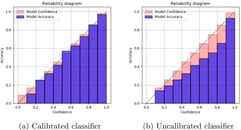
P( ˆY =y|pˆ=p) = p, ∀p∈[0,1] (3.17) Calibration can be treated as an additional piece of information, which makes it possible for a human user to decide how accurate the model is on a particular prediction. Model calibration can be visualized using calibration curves or reliabil-ity diagrams. For a well calibrated classifier, the relationship between prediction confidence and model accuracy is linear and is referred to as the ideal calibration line. The calibration error is the amount of deviation of the classifier’s calibration curve from the ideal calibration line. In a reliability diagram as displayed in Fig.

(31)

3.1, model prediction confidence on different input samples are grouped into interval bins and plotted along with the model accuracy per bin.

(a) Calibrated classifier (b) Uncalibrated classifier

Figure 3.1: Reliability diagrams illustrating the difference between a calibrated classifier (Fig. 3.1a) and an uncalibrated classifier (Fig. 3.1b) with confidence and accuracy on the x and y axis respectively. Note the linear relationship between confidence and accuracy for a calibrated classifier (Fig. 3.1a).

There exists several classifier post-calibration techniques which make slight modi-fications to the predicted confidence values so that the classifier’s calibration curve is as close as possible to the ideal calibration line, i.e., resulting in minimal calibration error. Histogram binning involves separating the prediction confidence values into several bins of fixed size and assigning an optimal calibrated confidence value for each bin [61]. Isotonic regression involves optimizing both the bin size and the calibrated confidence value per bin. Thus, the calibrated confidence value per prediction is determined by the bin to which the prediction confidence value belongs [62]. Platt scaling is a calibration technique introduced in the context of SVM classifiers which employs a logistic regression model on top of the classifier [43]. Here, the input to the logistic regression model are the prediction probabilities from the classifier and the outputs are calibrated prediction probabilities. The parameters of the logistic regression model are optimized using the validation set.

In the context of deep learning based classification models, Guo et al. [22] introduced a simple temperature scaling method. These models are hierarchical

(32)

models where the output from one layer is fed as input to following layer. The last layer of the model has as many number of logits as the number of classes in the dataset, followed by a softmax linearity. The softmax function is responsible for rescaling the logit values into a number between 0 and 1, hence is often used to quantify per class model prediction confidence. Temperature scaling involves scaling the logit values from the last layer by a temperature constant T before they are fed to the softmax function. This has an effect of reducing the over-confident predictions previously made by softmax. Since all logit values are scaled by the same temperature constant, the peak of the softmax function is not affected. Hence, temperature scaling does not modify the model accuracy but prevents over-confident predictions.

3.2.3 Selective classification

Selective classification is the process in which a classifier has the ability to abstain from making predictions on certain instances of the dataset in order to reduce the risk of misclassification. The empirical risk of a selective classifier f :X → Y [17], which defines a mapping over the m data-points X to thek class labelsY is given as follows, ˆ r(f, gθ) = 1 m Pm i=1l(f(xi), yi)gθ(xi) 1 m Pm i=1gθ(xi) (3.18) From Eq. (3.18) it is seen that the empirical risk of the selective classifier differs from the conventional classifier by the use of the selection function gθ(x). The selection function is responsible for allowing the classifier to make a prediction on a particular data-point and therefore its value is either 0 or 1,

gθ(x) =    1 if κf(x)≥θ; 0 otherwise. (3.19)

In the above equation, κf(x) refers to the confidence function used to give the final prediction confidence on the input data-points. This allows to use different confidence functions from MC dropout, ensembles or any other method discussed above other than the softmax. The prediction threshold θ is used so that only those data-points

(33)

are considered for classification whose confidence score are above this threshold. In order to obtain a low risk, it is important to have a good classifier f which does not have many misclassifications and a good threshold (θ) value so that the selection function gθ(x) is able to reject the data-points that are misclassified by

f. Geifman et al. [18] uses a combination of snapshots of the model from various training epochs rather than just the last model after training. This is because the last model does not provide reliable confidence estimates and is often over-confident in its predictions [13]. Geifman et al. [18] attributes this problem to the dynamics of the training process, where the model is able to produce high confidence scores for easy instances and low confidence scores for difficult instances during the early training epochs. However, as the training continues, the weights are further optimized so that the confidence estimates of the difficult instances are improved. At this point, the easy instances are ignored by the model since it only concentrates on the difficult instances, thereby making over-confident predictions on the easy instances. In order to address this issue, a fixed number of evenly spaced snapshots of intermediate models through the training epochs are taken and the confidence function κf is the average of these snapshots. An appropriate value forθ which gives the least risk for maximum coverage can be inferred from the Risk-Coverage (RC) curves where the risk and coverage are given by the numerator and denominator of Eq. (3.18).

Selective classification is able to improve the performance of other uncertainty estimation methods such as MC dropout [14], and deep ensemble [34]. However, it comes at an additional cost of requiring to save intermediate models during training as well as increased inference time because predictions from all these models are required for a test data-point.

(34)

(35)

4 Methodology

This chapter describes the experimental setup used to assess some of the uncer-tainty estimation methods discussed in the previous chapter. The different model architectures and datasets used to evaluate the uncertainty estimates produced by these methods are described in detail here.

4.1 Datasets

The evaluation procedure consists of experimentation with standard image classi-fication datasets such as CIFAR-10 and CIFAR-100 [32] followed by two other custom datasets. CIFAR-10 is a balanced dataset consisting of 60000 low resolution images belonging to 10 different classes. Each image is of size 32×32×3 and there are 6000 images per class. The images are by default split into a training set with 50000 images and a test set with 10000 images. We further make a training-validation split with a validation set consisting of 5000 images and the training set reduced to 45000 images. CIFAR-100 is also a balanced dataset, however it has 60000 high resolution images belonging to 100 different classes, with each class consisting of 600 images. The image dimensions and the train-validation-test split are similar to CIFAR-10. Evaluation on the CIFAR-100 dataset is important because the images are very similar to many real world datasets and it is highly likely that an algorithm performing well on this dataset will produce similar results on other real world datasets. The CIFAR-10 dataset, on the other hand is more akin to a toy dataset which is used for preliminary quick evaluation of algorithms.

(36)

(a) CIFAR-10 truck (b) CIFAR-100 pickup van

Figure 4.1: Fig. 4.1a showing more pixelated image 10 image than a CIFAR-100 image in Fig. 4.1b

For evaluating the performance of uncertainty estimation methods on real world problems, we use the Bosch optical inspection dataset which consists of 62814 gray-scale images belonging to 2 classes -OK and NOK- indicating the success/failure of the manufacturing process. The images in the dataset are scaled down to a size of 128×128. The dataset is highly imbalanced as there are only 3232 images which belong to the NOK class. Class balancing is done while training the model. The training set consists of 50246 images, while the validation and test set consists of 6281 and 6287 images.

(a) (b) _(c) _(d) _(e) (f) _(g)

(h)

(i) (j) (k) (l) (m) (n) (o) (p)

Figure 4.2: Sample image from each of the 16 classes in the RoboCup@Work dataset [38].

Additional evaluation is also performed on RoboCup@Work dataset consisting of images of tools used in the RoboCup@Work League [31]. The objects belong to 16 different classes as shown in Fig. 4.2, and out of the total 21706 images, 17358 are used for training, 2170 for validation, and 2178 for testing.

(37)

Chapter 4. Methodology

4.2 Models

Convolutional Neural Networks (CNN) have enjoyed great success after their superior performance in ImageNet Large Scale Visual Recognition Competition (ILSVRC) [49]. While a major factor for the success of CNNs is the availability of powerful hardware resources such as GPU’s, it is also important to note that new model architectures and ideas have boosted their performance. The different uncertainty estimation methods are evaluated on three popular standard deep learning architectures - VGG-16 [53] model, Wide-ResNet model [63], and Xception model [10]. The first two are used for classifying the standard CIFAR-10 and CIFAR-100 datasets, while the Xception model is used for the optical inspection and RoboCup@Work dataset. The weights of all layers of all three models are initialized using Glorot initialization [19].

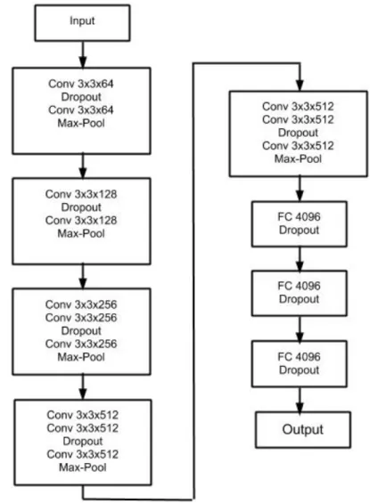
The VGG-16 model consists of 16 convolutional layers and 3 fully connected layers as shown in Fig. 4.3. The dropout layers are placed in between the convolutional layers (in short conv layers) and after the dense layers, having a dropout probability of 0.2 and 0.5, respectively. The model is trained for 160 epochs with a batch size of 128 using Stochastic Gradient Descent with Nesterov momentum as an optimizer with a learning rate and momentum of 0.01 and 0.9 respectively. The learning rate is decayed by a factor of 10 after 50, 80 and 110 epochs. Minor changes in those parameters are made in order to use the same architecture for evaluating the various uncertainty estimation.

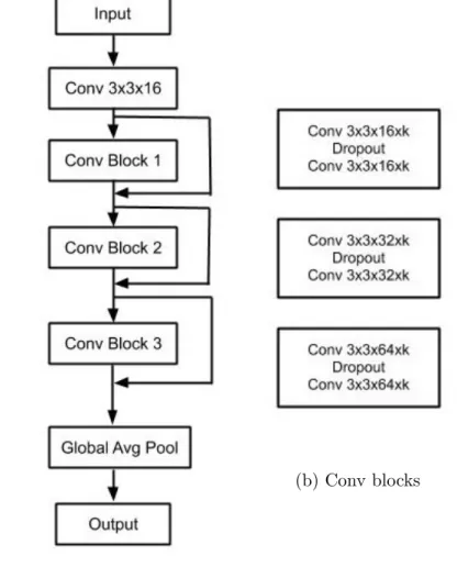
The Wide-ResNet-28-8 model as shown in Fig. 4.4 is used for classification of the CIFAR-10 and CIFAR-100 datasets with the same parameters. It has 4 convolutional blocks, where each block consists of convolutional layers followed by relu non-linearity, dropout layers, and a residual connection connecting the input and output of the block. The architecture is more memory efficient as it has fewer but wider layers compared to other architectures such as Inception and ResNet, and it also retains the benefits of residual connections. The total number of convolutional layers in the model, including the average global pooling and output layer is 28, while the 3x3x16 kernels are expanded by a width factor of 8. The model is able to achieve a higher accuracy compared to the VGG-16 model because of the presence of wider kernels. It uses a dropout rate of 0.3 and weight decay of 0.0005. The initial convolutional layer

(38)

Figure 4.3: VGG-16 architecture used for classifying images in CIFAR-10 and CIFAR-100. The conv layers in the architecture diagram represent the combination of convolution layer, batch-norm layer and relu non-linearity.

is followed by three convolutional blocks, where each contains 4 pairs of convolutional layers. The model is trained with Adam and a learning rate of 0.001 with a batch size of 128 for 110 epochs. The learning rate is decayed to 0.0001 and 0.00001 after 50 and 80 epochs.

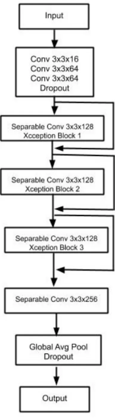
The Xception architecture consists of point-wise 1×1 convolutions followed by spatial 3×3 convolution. It is an extreme version of the Inception module [55] with the cross-channels correlations and the spatial correlations are entirely decoupled. A miniature version of the Xception architecture in contrast to the full architecture

(39)

(a) Wideresnet-28-8 architecture

(b) Conv blocks

Figure 4.4: Fig. 4.4b expands the conv blocks used in Fig. 4.4a. The width factor k is 8 and N is 4 in Fig. 4.4b. Each conv layer is a combination of convolution layer, batch-norm layer and relu non-linearity.

presented in Chollet [10] is used to solve our classification problem on the optical inspection dataset. The model consists of 3 Xception blocks with each Xception block containing 3 separable convolutional layers with intermediate relu non-linearities and dropout layers as shown in Fig. 4.5. The separable convolutional layers constitute the combination of point-wise 1×1 convolutions followed by depthwise 3×3 convolutions. The model uses a dropout rate of 0.4 and weight decay of 0.0005. The model is trained for 3 epochs with a batch size of 64 using Adam as an optimizer with a learning rate of 0.0001. The RoboCup@Work dataset uses the same model but with

(40)

minor changes in the following parameters. Stochastic Gradient Descent is used for training the model for 100 epochs with a learning rate of 0.01 and a Nesterov momentum of 0.9. Learning rate decay is used to reduce the learning rate to 0.0001 and 0.00001 after 50 and 80 epochs. All models are trained on one Nvidia Geforce GTX 1080 GPU except for the optical inspection dataset which requires two GPUs due to larger images of size 128× 128.

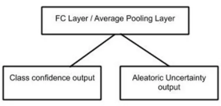
The choice of these architectures is primarily based on the presence of dropout layers in each of these models because uncertainty estimation using the MC dropout (MCD) method requires the presence of dropout layers in the model. The ensemble method (EN) uses the above described models with exactly the same parameters. On the other hand, the dropout layers are turned on during test time for MC dropout (MCD). Similarly for test time augmentation (TTA), the same model is evaluated but with several augmented test set images. Several meaningful augmentations are drawn from a set of image augmentations such as flipping, rotating, cropping, shifting, and brightness and contrast variations. The aleatoric uncertainty estimation method (MCDA) requires substantial changes to the model architecture and loss function. The last output layer of the model is split into two nodes - one for per class prediction confidence and the other for aleatoric uncertainty estimate as shown in the Fig. 4.6. The loss function used in [29] jointly optimizes the parameters of the model so as to produce proper uncertainty estimates along with class confidence scores.

A final note on this chapter is that all implementations of the above architectures and methods are done using a python Keras framework with Tensorflow backend.

(41)

(a) Xception architecture

(b) Xception block composition

Figure 4.5: Fig. 4.5b expands the Xception blocks used in Fig. 4.4a. All Xception blocks have convolutional and dropout layers with the same parameters. Each conv layer is a combination of convolution layer, batch-norm layer and relu non-linearity.

(42)

Figure 4.6: Second last layer of the models (Fully connected layer in case of VGG and average pooling layer in the case of Wideresnet and Xception) branches out into two nodes

(43)

5 Experimental Evaluation

This chapter focuses on the evaluation of different uncertainty estimation meth-ods - MC dropout (MCD) [14], deep ensembles (EN)[34], test time data augmenta-tion (TTA) [5], the combinaaugmenta-tion of MC dropout and test time data augmentaaugmenta-tion (MCD+TTA) [59] and MC dropout with Aleatoric loss (MCDA) [29] - used to address the overconfidence problem. These methods are applied to the various models and datasets discussed in the previous chapter. A per class output distribution of the softmax confidence is produced by these methods rather than a single point estimate for each test image. The resulting classifiers are evaluated on three aspects,

• classifier performance

• calibration

• sharpness

We aim to find the best uncertainty estimation method that is able to improve or maintain the classifier performance, and capture predictive uncertainty in a significant number of test set samples, while maximizing calibration.

(44)

5.1 Metrics

5.1.1 Sharpness Metrics

Uncertainty estimation techniques are able to reduce the sharpness of the overcon-fident predictions by producing a predictive distribution instead of point estimates. A predictive distribution is obtained for each image in the test set from the N forward passes (in MCD or TTA) or the N members of the ensemble. The sharpness of the predictive distribution is inversely proportional to produced uncertainty. The mean softmax confidence per class is computed from the predictive distribution and is used in the metric computation. The following metrics are used to measure the spread of the predictive distributions (for more details on the following metrics refer Chap. 2 of Murphy [40]), thereby directly yielding the uncertainty estimates per prediction made by the classifier.

1. Entropy : Entropy in general is used to measure the disorder/uncertainty of a random variable with some probability distribution [51]. The entropyH[ˆy|x, w] of the predicted softmax confidence ˆy with a probability distribution p from a model with weights wfor input image x, over each of the N forward passes or

N models in the ensemble [7] is represented as follows,

H[ˆy|x, Dtrain] =−X c (1 N X n p(ˆy=c|x, w)log(1 N X n p(ˆy=c|x, w))) (5.1)

Here, the number of realizations of the predictions ˆy is equal to the number of classes c.

2. Cross-Entropy : Another closely related measure is the cross-entropy. It measures the difference between the true distribution of the random variable and another distribution which approximates the true distribution. The ap-proximating distribution is given by the predictive distribution consisting of predicted confidences ˆy for all N forward passes/models in the ensemble, while the true class labelsy are represented using the indicator variable ✶(y ==c)

(45)

Chapter 5. Experimental Evaluation for class c[7]. H[y,yˆ|x, Dtrain] =−X c (1 N X n ✶(y== c)log(1 N X n p(ˆy=c|x, w))) (5.2)

It is also popularly called as the negative log loss in machine learning literature and is used to measure the performance of a classifier.

3. Mutual Information : Mutual information measures how much one random variable depends on another random variable. The mutual information between the predicted labels ˆy and the stochastic variable s for each of the methods, such as the weights of the network for MCD [16], the data augmentations applied during test time for TTA or the models of the models with different weights for EN, gives the measure of uncertainty. The greater the mutual information between the predicted labels and the stochastic variable, the higher the uncertainty. I[ˆy, s|x, Dtrain] =H[ˆy|x, Dtrain]− 1 N X n X c (−p(ˆy=c|x, s).log(p(ˆy=c|x, s))) (5.3) 4. Variance : Variance is another measure which is used to estimate the spread of predicted confidences from each forward pass/models in the ensemble. The per class prediction variance is given by the squared absolute difference between each per class predicted confidencep(ˆy=c|x, w) and the mean of all per class predictions from theN forward passes/models in the ensemble [16].

σ= 1 N X n ((p(ˆy=c|x, w))− 1 N X n p(ˆy=c|x, w))2 (5.4)

5.1.2 Classifier Performance Metrics

Classifier performance metrics are used to evaluate the performance of the classifier in correctly classifying samples from the test set (according to their true labels), when using uncertainty estimation methods. They measure the ability of the classifier to discriminate between samples from various classes.

(46)

• Accuracy: Accuracy is defined as the ratio of number of correct predictions to the total number of predictions [40]. It denotes the level of agreement between the predictions and the true labels. A difference between the model predictions and the true label results in a misclassification. Accuracy is representative of the misclassification rate of the model, i.e., lower the misclassification rate, the greater the accuracy. In our context, accuracy can be used to select an uncertainty estimation method which yields the lowest misclassification rate.

Acc= N o. of correct predictions

T otal no. of predictions (5.5)

• Excess-AURC : AURC represents the Area Under the Risk Coverage curves [18]. The risk ˆr(f, gθ) of a classifier f for a given coverage can be calculated according to Eq. 3.18 in Chap. 3. Eq. 5.6 and Eq. 5.7 are used to cal-culate and compare the AURC curves for the classifier using an uncertainty estimation methodAU RC(κ, f|Vn) and the baseline classifier AU RC(κ∗, f|Vn) respectively, by varying the coverage of the test set Vn withn data-points. The baseline classifier refers to a single trained deep learning model without any uncertainty estimation method applied to it.

AU RC(κ, f|Vn) = rˆ(f, gθ)|Vn n (5.6) AU RC(κ∗, f|Vn) = 1 n ˆ rn X i=1 i n(1−rˆ(f, gθ) +i) (5.7) E-AU RC =AU RC(κ∗, f|Vn)−AU RC(κ, f|Vn) (5.8) Excess-AURC is the difference between the AURC of the baseline classifier and that of the classifier using the uncertainty estimation method [18]. This metric is a unit-less measure which gives a bounded value between 0 and 1.

(47)

Chapter 5. Experimental Evaluation

5.1.3 Calibration Metrics

Calibration metrics assess the consistency of the classifier in producing reliable predictions. The degree of linearity between the predictive confidence and accuracy is directly proportional to calibration quality. Calibration metrics capture the deviations between accuracy and the predicted confidence, when they do not follow a linear relationship. The following metrics will be used to assess the calibration of the predictions produced by the deep learning classifier using the uncertainty estimation techniques.

1. Expected Calibration Error (ECE): It is the expected difference between the model accuracy and the predictive confidence p(ˆy=c|x, w) (for the true classcof the sample) [22]. This can also be visualized in the reliability diagrams as the gap between the model’s calibration curve and the ideal calibration line (Fig. 5.8).

ECE =_E(P(ˆy=c|p(ˆy=c|x, w))−p(ˆy =c|x, w)) (5.9) In the above equation, the first term denotes the frequency of correct predictions made by the model (accuracy).

2. Maximal Calibration Error (MCE): Maximal Calibration Error represents the maximum deviation between the model’s accuracy and the predictive confidence [22].

M CE =max(P(ˆy=c|p(ˆy=c|x, w))−p(ˆy=c|x, w)) (5.10)

3. Brier score : Brier score measures the closeness of the model’s predictive probability to true class probability (which is always 1). A good Brier score value is very close to zero as the squared difference between the true class probability (✶(y==c)) and the predicted confidence (p(ˆy=c|x, w)) is less. It

(48)

is a measure of both the classifier’s discriminative power and calibration [3]. BS = 1 N N X t=1 (p(ˆy =c|x, w)−✶(y==c))2 _(5.11)

5.2 Comparison Based on Uncertainty Quality

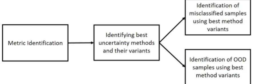
This experiment consists of four parts as illustrated in Fig. 5.1. Section 5.2.1 involves identifying the metric that is able to most distinctly represent the uncertainty in the predictions. Section 5.2.2, on the other hand consists of utilizing the identified metric to find out the best method that is able to reduce the sharpness of the deep learning classifier’s overconfident predictions. Section 5.2.3 aims to find the best method that identifies the maximum number of misclassifications as uncertain. Finally, Section 5.2.4 provides the results of evaluating the models with uncertainty estimation methods on data which does not belong to training distribution, called Out Of Distribution (OOD) datasets.

Figure 5.1: Workflow for comparative evaluation of different uncertainty estimation methods based on uncertainty quality

5.2.1 Metric identification

The uncertainty in the predictions is estimated using the various sharpness metrics described in Section 5.1.1. The aim of this experiment is to identify the best metric that is able to represent a greater spread given a particular uncertainty estimation method, dataset, and model. In order to evaluate the quality of these metrics, we utilize the concept of rank histograms, a diagnostic tool which is used to assess the

(49)

Chapter 5. Experimental Evaluation

spread of ensemble predictions in weather forecasting [45]. Originally, rank histograms consists of intervals/bins of sorted predictions from different ensemble members along the x-axis and the relative frequency of an observation falling into the bins on the y-axis. The reliability of the ensemble forecast is verified by repeatedly conforming if the real observations fall into one of the bins. If all bins contain approximately an equal number of predictions then the rank histogram is flat, thereby indicating the reliability of the ensemble forecast. On the other hand, deviations from a flat rank histogram are indicative of too much bias or variance exhibited by the ensemble [23].

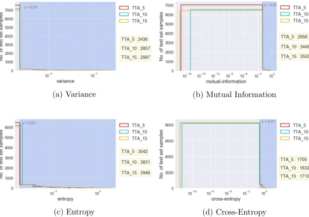
Rank histograms are adapted to our context of identifying uncertainty metrics by retaining their structure while giving them a new interpretation. We use the actual structure of rank histograms by ordering the model’s predictions into 100 bins with the x-axis scaled by the uncertainty metrics in ascending order, and the number of samples in the test set that fall into these bins on the y-axis. The rank histograms as shown in Fig. 5.2 are highly right skewed with most of the samples having close to zero values for all the uncertainty metrics. This can be explained by the fact that deep learning models produce highly over-confident predictions which provide very small values of uncertainty. Since our aim is to identify the uncertain predictions made by the model, a particular threshold value is chosen and samples that fall beyond this threshold are considered to be uncertain. The choice of 99 percentile area is made as compared to 97.5 or 95 percentile here because the distribution is highly right skewed and most of the samples are concentrated close to zero for all four metrics. However, it is important to note that the shape of the rank histograms is highly dependent on the model and dataset and does not exihibit the right skewness always.

Rank histograms can be plotted for all methods evaluated on all datasets with one of the four sharpness metrics on the x-axis and the number of test set samples on the y-axis. Fig. 5.2 shows the rank histograms plotted for the predictions from the VGG-16 used to classify images in CIFAR-10 test set with TTA as the uncertainty estimation method. The number of test samples that fall in the last 99 percentile area (i.e., the shaded region in Fig. 5.2) are counted for different metrics. The greater the number of samples that fall in the shaded region of the histogram, the better is the metric in capturing the spread of the distribution.