UC3M Working Papers
Statistics and Econometrics
17-06
ISSN 2387-0303
May 2017
Departamento de Estadística
Universidad Carlos III de Madrid
Calle Madrid, 126
28903 Getafe (Spain)
Fax (34) 91 624-98-48
Robust and Sparse Estimation of
High-dimensional Precision Matrices via Bivariate
Outlier Detection
Ginette Lafit
a, Francisco J. Nogales
bAbstract
Robust estimation of Gaussian Graphical models in the high-dimensional setting is
becoming increasingly important since large and real data may contain outlying
observations. These outliers can lead to drastically wrong inference on the intrinsic
graph structure. Several procedures apply univariate transformations to make the data
Gaussian distributed. However, these transformations do not work well under the
presence of structural bivariate outliers. We propose a robust precision matrix estimator
under the cellwise contamination mechanism that is robust against structural bivariate
outliers. This estimator exploits robust pairwise weighted correlation coefficient
estimates, where the weights are computed by the Mahalanobis distance with respect to
an affine equivariant robust correlation coefficient estimator. We show that the
convergence rate of the proposed estimator is the same as the correlation coefficient
used to compute the Mahalanobis distance. We conduct numerical simulation under
different contamination settings to compare the graph recovery performance of different
robust estimators. Finally, the proposed method is then applied to the classification of
tumors using gene expression data. We show that our procedure can effectively recover
the true graph under cellwise data contamination.
Keywords:
Gaussian Graphical Models; Cellwise Contamination; Robust Correlation
Estimation; Winsorization
a Department of Statistics, Universidad Carlos III de Madrid.
b Department of Statistics and UC3M-BS Institute of Financial Big Data, Universidad Carlos III de
Robust and Sparse Estimation of
High-dimensional Precision Matrices via Bivariate
Outlier Detection
Ginette Lafit∗
Department of Statistics, Universidad Carlos III de Madrid and
Francisco J. Nogales Department of Statistics and
UC3M-BS Institute of Financial Big Data, Universidad Carlos III de Madrid
Abstract
Robust estimation of Gaussian Graphical models in the high-dimensional setting is becoming increasingly important since large and real data may contain outlying obser-vations. These outliers can lead to drastically wrong inference on the intrinsic graph structure. Several procedures apply univariate transformations to make the data Gaus-sian distributed. However, these transformations do not work well under the presence of structural bivariate outliers. We propose a robust precision matrix estimator under the cellwise contamination mechanism that is robust against structural bivariate out-liers. This estimator exploits robust pairwise weighted correlation coefficient estimates, where the weights are computed by the Mahalanobis distance with respect to an affine equivariant robust correlation coefficient estimator. We show that the convergence rate of the proposed estimator is the same as the correlation coefficient used to compute the Mahalanobis distance. We conduct numerical simulation under different contamination settings to compare the graph recovery performance of different robust estimators. Fi-nally, the proposed method is then applied to the classification of tumors using gene expression data. We show that our procedure can effectively recover the true graph under cellwise data contamination.
Keywords: Gaussian Graphical Models; Cellwise Contamination; Robust Correlation Esti-mation; Winsorization.
∗
Ginette Lafit is Ph.D. student, Department of Statistics, Universidad Carlos III de Madrid (E-mail: [email protected]). Francisco J. Nogales is Associate Professor, Department of Statistics and UC3M-BS Institute of Financial Big Data, Universidad Carlos III de Madrid (E-mail: [email protected]). The research of Ginette Lafit and Francisco J. Nogales was funded by the Spanish government project MTM2013-44902-P.
1
Introduction
We consider the problem of estimating high-dimensional undirected graphs when the data possibly contains anomalies that are difficult to visualize and clean. Given nindependent samples of a p-dimensional random vector X = (X1, . . . , Xp), we can represent the
lin-ear dependency between variables by an undirected graph. The conditional dependence structure of the distribution can be represented by a graphical model, G = (V, E), where V ={1, . . . , p} is the set of nodes andE the set of edges inV ×V. The undirected graph establishes that if the variablesXiandXj are connected, then they are adjacent (Lauritzen,
1996). Statistically, we can measure linear dependencies by estimating partial correlations to infer whether there is an association between a pair of variables, conditionally on the rest of them. Furthermore, we can relate the nonzero entries in the precision matrix, de-noted by Ω = (ωij), with the nonzero partial correlation coefficients (Edwards,2000). This
procedure is known as covariance selection and is widely used to identify the conditional independence restrictions in an undirected graph (Dempster,1972). In particular, under a Gaussian distribution, the nonzero entries of the precision matrix imply that each pair of variables is conditionally dependent when controlling for the rest of them. These are known in the literature as Gaussian Graphical Models (GGMs) (Lauritzen,1996).
In a high-dimensional framework, the estimation of Ω is not straightforward because of the lack of a pivotal estimator such as the empirical covariance matrix. Moreover, when the dimensionpis larger than the number of available observations, the sample covariance matrix is not invertible. And even when the ratio p/n is approximately (but less than) one, the sample covariance matrix is badly conditioned and its inverse tends to amplify the estimation error, which can be observed by the presence of small eigenvalues (Ledoit and Wolf, 2004). From the asymptotic point of view, when both n and p are large (i.e. p=O(n)), the sample covariance matrix is not a consistent estimator (El Karoui,2008). To deal with this problem, several covariance selection procedures have been proposed based on the assumption that Ω is mostly composed by zero elements. This suggests that even when p = O(n) the dimension of the problem may still be tractable since the number of
edges will grow more slowly than the number of observations (Meinshausen and B¨uhlmann, 2006).
Several precision matrix estimators have been proposed in the literature. Meinshausen and B¨uhlmann(2006) propose the neighborhood selection procedure that consistently esti-mates sparse high-dimensional graphs by estimating a lasso regression for each node in the graph. Peng et al.(2009) present a procedure that simultaneously performs neighborhood selection for all variables to estimate joint sparse regressions, applying an active-shooting to solve the lasso. Yuan(2010) replaces the lasso regression with a Dantzig selector. Liu and Wang(2012) propose an asymptotically tuning-free procedure that estimates the precision matrix in a column-by-column fashion. Zhou et al. (2011) propose an estimator for the precision matrix base on an`1 regularization and thresholding to infer a sparse undirected graphical model. Ren et al. (2015) propose a nodewise regression approach to obtain as-symptotically efficient estimation of each entry of the precision matrix under sparseness conditions.
Penalized likelihood methods have also been introduced for estimating sparse precision matrices. Yuan and Lin (2007) propose to estimate the precision matrix by penalizing the log-likelihood function. Convex and fast algorithms were developed byBanerjee et al. (2008) and Friedman et al. (2008). Friedman et al. (2008) propose the Graphical lasso (Glasso) procedure to estimate sparse precision matrices fitting a modified lasso regression to each variable and solving the problem by a coordinate descent algorithm. Lam and Fan (2009) and Fan et al. (2009) propose methods to diminish the bias imposed by the `1 penalty by introducing a non-convex SCAD penalty. Cai et al. (2011) estimate preci-sion matrices for both sparse and non-sparse matrices, without imposing a specific sparsity pattern solving the dual of an `1 penalized maximum likelihood problem. Consistency of penalized likelihood procedures were also explored. Rothman et al.(2008) estimate conver-gence rates under the Frobeniuos norm andYuan and Lin(2007), Ravikumar et al.(2008) and Ravikumar et al.(2011) estimate convergence rates for subgaussian distributions.
well suited to handle noisy data (contaminated by outliers). The existing approaches to estimate the precision matrix and recover the support of the GGM use as input the em-pirical covariance matrix. The emem-pirical covariance and correlation matrix estimates are very sensitive to the presence of multidimensional outliers (Alqallaf et al.,2002). The vi-olation of the Gaussian assumption may result in poor recovery of the GGM and biased estimation of the precision matrix (see Finegold and Drton, 2011; Liu et al., 2012; Sun and Li,2012). In the high-dimensional setting, the fraction of perfectly observed rows may be very small. If all components of a row have an independent chance of being contami-nated, then the probability that a case is perfectly observed is small. Alqallaf et al.(2009) propose a contamination model where the contamination in each variable is independent from other variables (i.e. componentwise outliers). It generalizes the classical Tukey-Huber row-wise contamination model (seeTukey,1962;Huber et al.,1964) and allows for cellwise contamination that can be applied to explain the contamination mechanism in Microarrays experiments (see Troyanskaya et al., 2001; Liu et al., 2003). The cellwise contamination model lacks the affine equivariant property. Henceforth, existing approaches for robust covariance estimation such as M-estimates (Maronna, 1976), Minimum Volume Ellipsoid (MVE) and Minimum Covariance Determinant (MCD) estimators (Rousseeuw,1985,1984) and the Stahel-Donoho (SD) estimators (Stahel,1981;Donoho,1982), may not be reliable in high-dimensional data sets since the operations to compute affine equivariant estimates tend to propagate the effect of multivariate outliers. Also, these estimators downweight contaminated observations to reduce their influence, which produces a significant loss of information whenn < p.
To deal with outliers in high-dimensional data sets, many procedures construct robust covariance and correlation matrices by using pairwise robust correlation coefficients. Liu et al. (2009) propose to apply a univariate monotone transformation to make the data Gaussian distributed. Then, a robust precision estimator of the correlation matrix can be computed from the transformed data. The estimated correlation matrix is plugged into the existing parametric procedures (the Graphical Lasso, CLIME, or graphical Dantzig
Se-lector) to obtain the final estimate of the inverse correlation matrix and the graph. Liu et al. (2012) and Xue et al. (2012) propose to estimate the unknown correlation matrix with robust nonparametric rank-based statistics Spearman’s rho and Kendall’s tau. Fine-gold and Drton(2011) propose to use multivariatet-distribution for more robust inference of graphs. However, there is not a direct relationship between the zero elements on the estimated precision matrix and the conditional independences when a t-distribution is as-sumed. Sun and Li(2012) propose a robust estimator of the GGM through`1-penalization of a robustified likelihood function. Ollerer and Croux¨ (2015) andLoh and Tan(2015) pro-pose robust precision matrix estimation under the cellwise contamination setting. These methods estimate robust pairwise scatter covariance using rank-based statistics and plug them into the existing parametric procedures. Ollerer and Croux¨ (2015), andLoh and Tan (2015) analyze the breakdown property of the Graphical lasso and CLIME.
The robust correlation matrix based on univariate transformations to achieve normality are not robust under the presence of structural bivariate outliers which could lead to a misleading graph support recovery. We propose an approach to robustly estimate a Gaus-sian Graphical Model when there is cellwise contamination in the data. Following the idea ofKhan et al. (2007), we estimate robust correlation coefficients applying a bivariate winsorization to the data given an affine equivariant robust correlation coefficient. This transformation allows us to identify bivariate outliers. The proposed correlation matrix is plugged into a parametric procedure to compute the precision matrix. We show that the bivariate winsorized pairwise correlation coefficient converges to the true parameter at the same rate as the affine equivariant correlation coefficient. This result suggests that if the robust correlation coefficient estimator, which is used to winzorize the data, converges to the true parameter at the optimal parametric rate, then the bivariate winsorized correla-tion matrix achieves the optimal parametric rate of convergence in terms of both precision matrix estimation and graph recovery.
Finally, we perform simulation studies and show that under different contamination set-tings our procedure outperforms the normal-score based nonpararnomal estimator proposed
by Liu et al. (2009) and the nonparanormal SKEPTIC proposed by Liu et al. (2012). We also apply our procedure to the classification of tumors using gene expression data. We show that our procedure achieves good classification performance. The empirical results suggest that, by using bivariate winsorization on the data based on some affine equivariant robust correlation estimate, we can efficiently recover the GGM under cellwise contamination.
The rest of the article is organized as follows. In the next section we briefly review the cellwise contamination model and the existing approaches to estimate robust precision matrices. In Section 3 we present the winsorized correlation matrix estimator, which is able to identify structural bivariate outliers under the cellwise contamination mechanism. In Section 4 we present a theoretical analysis of the method. In Section 5 we present numerical results on simulated data under different contamination mechanisms. Section 6 presents the results based on real data where the problem is the classification of tumors using gene expression data. Finally, we discuss the connections to existing methods and possible future directions.
2
Problem Setup
In this Section we consider the problem of estimating a high-dimensional undirected graph when the data possibly contains anomalies that are difficult to visualize and clean. A robust statistic must be able to efficiently model the bulk of data points, be resistant to model deviations, and to perform well under the correct model. The performance of a robust estimator can be analyzed with contamination or mixture models. We introduce a general contamination model able to capture properties of high-dimensional outliers, gross errors or missing values, among other perturbed observations. In high-dimension, the fraction of perfectly observed rows may be very small. To deal with this issue, Alqallaf et al. (2009) propose a contamination model where the contamination in each variable is independent from other variables (i.e. componentwise outliers).
with mean µ and correlation matrix Γ = (ρij). The linear dependency between variables
are represented by an undirected graphG= (V, E), whereV ={1, . . . , p}is the set of nodes and E the set of edges inV ×V. The contamination model can be written as follows:
Y= (I−B)X+BZ (2.1)
where I is a p×p identity matrix, Z ∈ Rp an arbitrary random vector and B is the contamination indicator matrix:
B= B1 0 · · · 0 0 B2 · · · 0 .. . ... . .. ... 0 0 · · · Bp (2.2)
and eachBj is a Bernoulli random variable withP(Bj = 1) =ε.
The classical contamination setting or row-wise contamination model, proposed by Tukey (1962) and extended by Huber et al. (1964), assume that B1, . . . , Bp are fully
de-pendent P(B1 = B2 = . . . = Bp) = 1. Then, the observed variable Y is a mixture of
two independent distributions. Under this model a fraction (1−ε) of the rows are multi-variate Gaussian distributed and a fraction εare outliers. Furthermore, the percentage of contaminated cases is preserved under affine equivariant transformations.
But the Tukey-Huber model does not adequately represent the reality of many multi-variate high-dimensional data sets. This model assumes that the majority of the cases are not contaminated. When p > n, downweighting an entire case may be inconvenient. The main drawback is that the probability of a perfectly observed row became very small when the number of variables increases (i.e. p=O(n)).
Alqallaf et al. (2009) propose an alternative model where the contamination in each variable is independent from other variables (i.e. componentwise outliers). In this model,
the variablesB1, . . . , Bp are independent:
P(B1 = 1) =. . .=P(Bp = 1) =ε (2.3)
Then, the probability of an outlier occurring in the each variable is the same. In this model the probability that a row is not contaminated is (1−ε)p, which decreases with p. This model allows for cellwise contamination and is denoted by fully independent contamination model.
The fully independent contamination model lacks of affine equivariance. Under the cellwise contamination, each column has on average (1−ε) of clean observations. Then, linear combinations of these columns produce an increment in the number of contaminated cases (i.e. outlier propagation). Henceforth, in the high-dimensional setting, robust affine equivariant methods are not robust against propagation of outliers.
Under the cellwise contamination model, a robust estimation of the precision matrix Ω can be obtained by plugging a robust correlation matrix estimator, denote by ˆΓ, into the following `1-regularized log-determinant program (see Ollerer and Croux¨ , 2015; Loh and Tan,2015):
ˆ
Ω = argmin Ω0
{tr(ΩˆΓ)−logdet(Ω) +λkΩk1,off} (2.4)
whereλ >0 is the regularizing constant of the off-diagonal `1 regularizer
kΩk1,off:=X
i6=j
|ωij| fori, j= 1, . . . , p (2.5)
Ravikumar et al.(2011) show that, for any positiveλand ˆΓ with strictly positive diagonals elements, the problem has a unique solution and the resulting matrix is positive definite (i.e. ˆΩ0).
Classical approaches for robust scatter estimation such as M-estimates (Maronna,1976), Minimum Volume Ellipsoid (MVE) and Minimum Covariance Determinant (MCD) esti-mators (Rousseeuw, 1985, 1984) and the Stahel-Donoho (SD) estimators (Stahel, 1981;
Donoho,1982), are not well suited when the contamination mechanism operates on individ-ual variables (columns) rather than individindivid-ual cases (rows). Under cellwise contamination each column in the data table contains on average a fraction of ε contaminated observa-tions. Classical affine equivariant estimators apply linear combination of the columns on the original data. This spreads the contamination in one of the cells of an observation over all its components.
To deal with high-dimensional cellwise outliers, Alqallaf et al. (2002) propose to use coordinated wise outlier insensitive transformations to estimate pairwise scatter estimates. These procedures operate one variable at a time and guarantee the protection against outlier propagation.
Let Y(1), . . . ,Y(n) be a sample of size n where Y(k) = (Y1(k), . . . , Yp(k))T ∈Rp fork = 1, . . . , n. Let’s assume that there exists an appropriate score function, denoted by fi(Yi),
that preserves monotone ordering and commute with permutations of the components of (Yi(1), . . . , Yi(n)). Huber(2011) defines the pairwise robust correlations coefficients through the Person correlation coefficient computed on the outlier free univariate transformed data. To estimate the robust pairwise correlation matrix, Liu et al. (2009) propose the non-paranormal model where the random vector Y = (Y1, . . . , Yp)T is replaced by the
trans-formed variablef(Y) = (f1(Y1), . . . , fp(Yp))T such thatf(Y) is multivariate Gaussian with
mean zero and correlation matrix denoted by Γnpn.
Let ˆFi(t) = n+11 Pnk=1I(Yi(k)) be the scaled empirical cumulative function of Yi. To
estimate the nonparanormal transformation, Liu et al. (2009) define the coordinated wise transformation function ˆfi(t) = Φ−1
Tδn[ ˆFj]
where Φ−1(·) is the standard Gaussian quan-tile function andTδn is a winsorization operator defined as
Tδn(y) = δn if Fˆi(y)< δn y if δn≤Fˆi(y)≤(1−δn) (1−δn) if Fˆi(y)>(1−δn), (2.6)
where δn = 4n1/4√1πlogn is a truncation parameter. The nonparanormal estimate of the correlation matrix is computed as follows
ˆ ρnpnij = 1 n Pn k=1fˆi(Yi(k)) ˆfj(Yj(k)) q 1 n Pn k=1fˆi2(Y (k) i )· q 1 n Pn k=1fˆj2(Y (k) j ) . (2.7)
Then, the precision matrix nonparanormal estimator is computed by plugging Γnpn into the `1 log-determinant program (2.4). Liu et al. (2009) establish convergence rate for estimating the precision matrix in the Frobenious and spectral norm when p is restricted to a polynomial order ofn.
Liu et al. (2012) show that rate of convergence of the nonparanormal estimator is not optimal. Liu et al. (2012) and Xue et al. (2012) present an alternative procedure that applies rank based methods to estimate the pairwise correlation matrix without computing explicitly the marginal transformations. This approach is called the nonparanormal SKEP-TIC and achieves the optimal parametric rate of convergence in terms of both precision matrix estimation and graph recovery.
Let r(ik) be the rank of Yi(k) among Yi(1), . . . , Yi(n) and ¯ri = 1nPnk=1r (k)
i = n+12 . The Spearman’s rho statistics can be computed as follows
ˆ ρρij = Pn k=1(r (k) i −r¯i)(r(jk)−¯rj) q Pn k=1(r (k) i −r¯i)2Pnk=1(r (k) j −¯rj)2 . (2.8)
The nonparanormal model implies that (fi(Yi), fj(Yj)) follows a bivariate normal
distribu-tion with correladistribu-tion parameterρnpnij . A classical result due toKendall and Gibbons(1990) and Kruskal (1958) shows that ρnpnij = 2sin π6ρρik. Henceforth, the correlation matrix of the nonparanormal model can be alternatively computed as follows:
ˆ ρSij = 2sin(π6ρˆρij) for i6=j 1 for i=j (2.9)
Liu et al. (2012) show that when the data contamination is low, the nonparanormal estimator is slightly more efficient than the nonparonormal SKEPTIC. But when the con-tamination increases the later siginificantly outperforms the normal-score based estimator proposed byLiu et al.(2009).
The main drawback of the univariate outlier insensitive transformations is their lack of robustness against structural outliers (see Alqallaf et al., 2009). This type of outliers can only be handled via robust affine equivariant methods. In the next section we propose an alternative robust pairwise correlation coefficient estimator that apply robust affine equivariant methods to the bivariate data. This method applies a bivariate winsorization that shrinks observations to the border of a tolerance ellipse so that outlying observations are appropriately downweight to obtain a robust correlation coefficient estimate that allows for protection against structural bivariate outliers.
3
The Proposed Winsorized Correlation Matrix
In this section, we propose to estimate the precision matrix by computing an affine equiv-ariant transformation to the bivariate data. This transformation takes into account the ori-entation of the bivariate data and allows for protection against structural bivariate outliers. Then, a pairwise correlation matrix is computed from the outlier free bivariate transformed data. The resulting correlation matrix is plugged into the `1 log-determinant divergence optimization problem defined in (2.4).
To obtain a correlation estimator that is robust against structural bivariate outliers we could apply affine equivariant bivariate M estimators (Maronna, 1976). However, in the high-dimensional setting we require fast robust correlation estimates. Following the idea of Khan et al. (2007), we estimate the robust correlation coefficients applying a bivariate winsorization to the bivariate data given an affine equivariant robust correlation coefficient. In order to compute a correlation matrix that is robust against bivariate outliers, we are going to use reweighted robust pairwise estimators of scatter, where the weights are
com-puted by the Mahalanobis distance with respect to an affine equivariant robust correlation estimator.
Let the vector XJ = (Xi, Xj)T, fori, j = 1, . . . , p, follow a bivariate Gaussian
distribu-tion with meanµJ = (µi, µj), covariance σJ2 = (σi2, σj2) and correlation matrix ΓJ. Let’s
compute the squared population Mahalanobis distance as follows
d2k = Y (k) i −µi σi ,Y (k) j −µj σj ! (ΓJ)−1 Yi(k)−µi σi ,Y (k) j −µj σj !T . (3.1)
We define the following weights
wk(d2k) = q c2/d2 k if d2k> c2 1 if d2 k≤c2 (3.2)
wherec2 is given byP r(χ22 > c2) =εandεis the proportion of outliers we want to control assuming that the majority of the data follows a bivariate Gaussian distribution.
Assuming we observe the vector of bivariate observations Y(Jk) =
Yi(k), Yj(k) T
for i, j = 1, . . . , p and k = 1, . . . , n, the following Proposition, due to Cerioli (2010), refers to the distribution of the Mahalanobis distance of the observations for whichwk = 1.
Proposition 1. The distribution of Y(Jk) conditioned on wk = 1 is a truncated bivariate
Gaussian distribution with
E(Y(Jk)|wk= 1) =µJ and Cor(Y (k) J |wk= 1) =κ −1 ε ΓJ (3.3) where κε= 1−ε P(χ2 2 > χ22,1−ε) . (3.4)
If we denotewε=Pnk=1wk and (ˆµεi,µˆεj) = 1 wε n X k=1 wkYi(k), 1 wε n X k=1 wkYj(k) ! (ˆσεi,σˆεj) = κε wε−1 n X k=1 wk(Yi(k)−µˆεi)2 !1/2 , κε wε−1 n X k=1 wk(Yj(k)−µˆεj)2 !1/2 ˆ ρεij = κε wε−1 n X k=1 wk Yi(k)−µˆεi ˆ σε i ! Yj(k)−µˆεj ˆ σε j ! , (3.5) then ΓˆεJ = ( ˆρεij) and wε/n = (1−ε) +Op(1/ √
n) and it follows that E( ˆµεJ) → µJ and E(ˆΓεJ)→ΓJ.
A direct result from Proposition 1 is that we can obtain consistent estimators of µJ
and ΣJ applying a bivariate winsorization to the observations of Y(Jk). To obtain robust
estimates against two-dimensional structural outliers we propose to estimate the Maha-lanobis distance using some affine equivariant robust correlation coefficient. To do that, we can definen bivariate standardized observations
Yi(k)−ˆµ0 i ˆ σ0 i ,Y (k) j −ˆµ0j ˆ σ0 j where ˆµ0i is a robust scale estimate and ˆσi0 is a robust location estimate. Now let ˆΓ0J = (ρ0ij) be a robust and affine equivariant correlation estimator of the correlation matrix ΓJ. We will use ˆΓ0J as a
diagnostic tool to identify two-dimensional structural outlying observations. If the initial robust estimator reflects the bulk of data, then the outlying observation will have a large Mahalanobis distance and the outlying observations could be downweighted in order to minimize their influence. We define the Mahalanobis distance estimate as follows:
d2k,Γˆ0 J = Y (k) i −µˆ0i ˆ σi0 , Yj(k)−µˆ0 j ˆ σ0j ! (ˆΓ0J)−1 Y (k) i −µˆ0i ˆ σi0 , Yj(k)−µˆ0 j ˆ σ0j !T . (3.6)
We propose two estimators to compute the correlation matrix ˆΓ0J and to perform the bivariate winsorization. First, we apply theAdjusted Winsorizationproposed byKhan et al. (2007). This approach takes into account the quadrants relative to the coordinatewise
medians and considers two tuning constants to perform univariate winsorization of the data. A larger tuning constantc1is used to winsorize the points lying in the two diagonally oppose quadrants that contains most of the standardize data. A smaller tuning constant c2 is used to winsorize the remaining data. We setc1 = 2 andc2=√hc1 whereh=n2/n1, n1 is the number of observations in the major quadrants and n2 = n−n1. The adjusted winsorization is then defined as (seeKhan,2006)
Ψ(Yi, Yj) = ψc1 Y i−ˆµ0i ˆ σ0 i , ψc1 Y j−ˆµ0i ˆ σ0 i if Yi−ˆµ0i ˆ σ0 i Yj−ˆµ0 j ˆ σ0 j ≥0 ψc2 Yi−ˆµ0 i ˆ σ0 i , ψc2 Yj−ˆµ0 i ˆ σ0 i if Yi−ˆµ0i ˆ σ0 i Y j−ˆµ0j ˆ σ0 j <0, (3.7)
whereψc(y) = min{max{−c, y}, c}is a non-decreasing symmetric function andc1andc2are
previous constants. Then, the correlation coefficient estimator ˆρ0J is obtained by computing the Pearson correlation on the adjusted winsorized data. In the second alternative, we compute ˆΓ0J using the Spearman’s rho as in equation (2.9). This approach is denoted by Spearman’s Winsorization.
Therefore, given an affine equivariant robust correlation estimator ˆΓ0J (i.e. Adjsuted Winsorized correlation coefficient or Spearman’s rho), we estimate the robust Mahalanobis distance as in equation (3.6), then the outlier-free bivariate transformed data is computed as follows ΨW(Yi(k)) = q c2/d2 k,Γˆ0 J Yi(k)−ˆµ0i ˆ σ0 i if d2 k,Γˆ0 J > c2 Yi(k)−ˆµ0 i ˆ σ0 i if d2 k,Γˆ0 J ≤c2, (3.8)
wherec2 is given byP(χ22 > c2) =εand εis the proportion of outliers we want to control assuming that the majority of the data follows a bivariate Gaussian distribution.
Given the observations (Y1(k), . . . , Yp(k))T, the winsorized correlation matrix ˆΓW = ( ˆρWij)
is obtained by computing the Pearson correlation coefficient with respect to the bivariate winsorized data. The robust precision matrix is estimated by plugging the winsorized correlation matrix ΓW into the`1 log-determinant divergence (2.4).
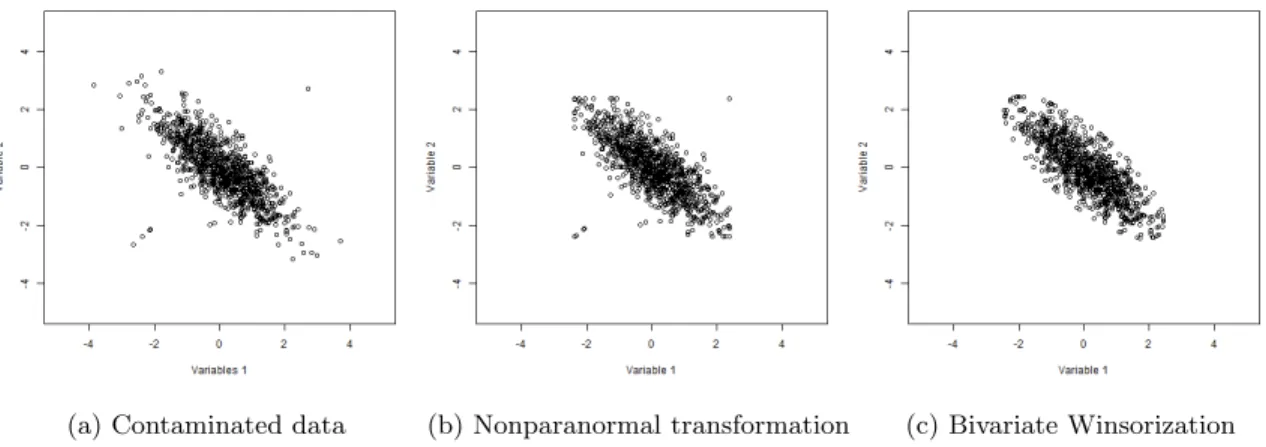
To show how the bivariate winsorization works under cellwise contamination, we simu-late data from a bivariate Gaussian distribution where the correlation is set equal to -0.8. We selectn= 1000 and generate 5 structural bivariate outliers. Figure 1, Panel (a), shows the scatter plot of contaminated data. Figure1, Panel (b), shows the scatter plot when we apply the non-paranormal transformation (seeLiu et al.,2009). The non-paranormal trans-formation shrinks the correlation outliers to the boundary of a square. However, it does not take into account the orientation of the data and the effect of the structural outliers is not significantly downweighted. In Figure1, Panel (c), we observe that the bivariate trans-formation shrinks the outliers to the boundary of an ellipse of equal Mahalanobis distance. Henceforth, the influence of the bivariate outliers, when we compute the robust correlation coefficient, is appropriately downweighted.
(a) Contaminated data (b) Nonparanormal transformation (c) Bivariate Winsorization
Figure 1: Illustration of nonparanormal tranformation and bivariate winsorization under bivariate contamination.
In the next section we state some analytical properties of the bivariate winsorized pair-wise scatter estimate is the same as the affine equivariant robust correlation estimates used to compute the Mahalanobis distance. This result suggests that if the initial robust corre-lation coefficient estimate converges to the true parameter at the optimal parametric rate,
then the winsorized precision matrix achieves the optimal parametric rates of convergence in terms of both precision matrix estimation and graph recovery.
4
Analytical Properties
In this section we establish some analytical properties for the proposed bivariate winsorized correlation estimator. The main conclusion drawn from the theoretical results is that the location and scatter estimates computed from the bivariate winsorized data have the same rate of convergence as the affine equivariant robust location and pairwise scatter estimates used to compute the Mahalanobis distance.
Let Y(1)J , . . . ,Y(Jn) be independent bivariate random vectors that follow a distribution in an elliptical family with density
f(yJ) = det(ΓJ)−1/2h Yi−µi σi ,Yj−µj σj T (ΓJ)−1 Yi−µi σi ,Yj −µj σj ! (4.1)
whereh : [0,∞)→[0,∞) is assumed to be known. Under the assumption that the vector
YJ = (Yi, Yi)T is bivariate Gaussian distributed, the function h corresponds to h(r) =
(2π)er/2. Moreover, we assume the following smoothness conditions on the functionh:
(H1) his continuous differentiable.
(H2) hhas finite fourth moment: R(yTJyJ)2h(yTJyJ)dyJ <∞.
Let ˆθ0 = (ˆµ0i,µˆ0j,σˆi0,σˆj0,ρˆ0ij) denote robust and affine equivariant estimators of location and scatter. We will use these estimates as diagnostic tool to identify structural bivariate outliers. Let ˆd2
k be the Mahalanobis distance computed as in (3.6). We apply the bivariate
transformation in (3.8) and we compute the bivariate winsorized correlation estimator ˆρWij. Let w : [0,∞) → [0,1] be the function defined in (3.2), that satisfies the following condition
We study the asymptotic behavior of ˆρWij as n → ∞. Let θ∗ = (µi, µj, σi, σj, ρij)
de-noted the true vector of parameters. Assuming that the estimates ˆθ0 are affine equivariant and consistent in probability (i.e. ˆθ0 → θ∗ in probability), the next Theorem analyzes the asymptotic properties of the bivariate winsorized correlation coefficient. The proof fol-lows the analysis for reweighted estimators of multivariate location and scatter ofLopuha¨a (1999).
Theorem 1. Let Y(1)J , . . . ,Y(Jn) be independent bivariate random vectors with parameter vector θ∗= (µi, µj, σi, σj, ρij) which are assumed to have density function defined in (4.1).
Suppose that w : [0,∞) → [0,1] satisfies (W) and h satisfies (H1) and (H2). Let θˆ0 be affine equivariant and consistent estimate in probability of θ∗. Then,
ˆ ρWij −c1ρij =op(1/ √ n) +op(ˆθ 0 −θ∗) +1 n n X k=1 ( w(d2k) Y (k) i −µi σi ! Yj(k)−µj σj ! −c1ρij ) , (4.2) where the constantc1 is given by
c1=π Z ∞
o
w(r2)h(r2)r3dr >0. (4.3)
Proof. Theorem 1 can be proved by adapting the proof in Lopuha¨a (1999). The Maha-lanobis distance can be written as a function of the vectorθ. Thus, we define the following functions Ψ1(yJ,θ) =w d2(θ) yJ Ψ2(yJ,θ,t) =w d2(θ) (yJ−t)(yJ−t)T. (4.4)
We define the bivariate adjusted winsorization estimates of location and covariance as follows ˆ µWJ = 1 n n X k=1 w ˆ d2k Y(Jk) ˆ ΣWJ = 1 n n X k=1 w ˆ d2k (Y(Jk)−µˆWJ )(Y(Jk)−µˆWJ )T. (4.5)
Then, ˆµWJ and ˆΣWJ can be written as: ˆ µWJ = Z Ψ1(yJ,θ)dPn(yJ) ˆ ΣWJ = Z Ψ2(yJ,θ,µˆWJ )dPn(yJ), (4.6)
wherePndenotes the empirical measure corresponding to Y(1)J , . . . ,Y(Jn).
Moreover, estimates in (4.6) can be written as:
Z Ψ1(yJ,θˆ 0 ) = Z Ψ1(yJ,θˆ 0 )dP(yJ) + Z Ψ1(yJ,θ∗)d(Pn−P)(yJ) + Z Ψ1(yJ,θˆ0)−Ψ1(yJ,θ∗) d(Pn−P)(yJ), (4.7)
Suppose that ΣJ = B2 where B belongs to the class of positive definite symmetric
matrices. Let ˆµ0J = (ˆµ0i,µˆj0)T and ˆΣ0J = Bn2 be affine equivariant location and scatter estimates such that ( ˆµ0J−µJ, Bn−B) are consistent in probability. Then, using the result
inLopuha¨a (1999) the first term in the right-hand side of (4.7) is c0( ˆµ0J−µJ) +op( ˆµ0J −
µJ, Bn−B) and the third term is op(1/
√
n). The second term is equal to: Z Ψ1(yJ,θ∗)d(Pn−P)(yJ) = 1 n n X k=1 w(d2k)(Y(Jk)−µJ). (4.8)
This proves the expansion for ˆµWJ :
ˆ µWJ −µJ = 1 n n X k=1 w(d2k)(Y(Jk)−µJ) +c0( ˆµ0J−µJ) +op(1/ √ n) +op( ˆµ0J−µJ,Σˆ0J−ΣJ) (4.9)
the constants are given by c0 = 2π Z ∞ o w(r2)[h(r2) +h0(r2)r2]rdr (4.10) c1 =π Z ∞ o w(r2)h(r2)r3dr >0. (4.11)
In a similar way, using that the expansion of ˆµWJ implies that ˆµWJ → µJ, it can be shown that Z Ψ2(yJ,θˆ 0 ,µˆWJ ) =c1ΣJ+c2{tr(B−1(Bn−B))ΣJ + 2B−1(Bn−B)ΣJ} + 1 n n X k=1 {w(d2k)(Y(Jk)−µJ)(Y(Jk)−µJ)T −c1ΣJ} +op(1/ √ n) +op( ˆµ0J−µJ, Bn−B,µˆWJ −µJ), (4.12)
whereB−1(Bn−B) = (Bn−B)B−1=An,An isop(1) and the constant c2 is given by
c2 =π Z ∞ o w(r2) r2h(r2) +r 4 2h 0(r2) rdr. (4.13)
Finally, let define the vector of standardized observations ˆyJ = Yi(k)−ˆµW i ˆ σW i ,Y (k) j −ˆµWj ˆ σW j T
The bivariate winsorized correlation matrix can be define as:
ˆ ΓWJ =
Z
Ψ2(ˆyJ,θ)dPn(ˆyJ). (4.14)
Using the result in (4.12) we obtain (4.2).
Theorem1shows that the bivariate winsorized correlation estimate ofρij works as well
as the affine equivariant robust estimator ˆρ0ij used to identify structural bivariate outliers. Hence, if ˆρ0ij converges at a rate slower than √n, then the bivariate winsorized estimator ˆ
ρWij converges toc1ρij at the same rate.
Spearmans’ rho as diagnostic tool to estimate the Mahalanobis distance and obtain robust-ness against two-dimensional outliers. Khan (2006) shows that under certain regularity condition, the correlation coefficient based on adjusted winsorized data is consistent and asymptotically normal. Liu et al. (2012) andXue et al. (2012) show that the Spearman’s rank correlation estimate is consistent and converge to ρij with the optimal parametric
rate.
Regarding the precision matrix estimator,Ravikumar et al.(2008) andRavikumar et al. (2011) study the sufficient condition on the estimated correlation matrix in order to achieve the optimal parametric rate in high-dimension. A sufficient condition to ensure consistency and graph recovery of the precision matrix estimator, at the minimax optimal rate, is given by the condition that the robust correlation matrix estimate ˆΓ converges to the true correlation matrix Γ at the optimal parametric rate (seeLiu et al.,2012;Xue et al.,2012). The following Lemma, adopted fromRavikumar et al.(2011), shows that if the bivariate winsorized correlation coefficient works as well as the usual sample correlation estimator based on uncontaminated data, then the bivariate winsorized correlation estimate achieves the optimal parametric rate.
Lemma 1. Assume there exists a constant C such that the robust bivarite winsorized cor-relation coefficient estimator satisfies the following concentration bound
P r(|ρˆWij −ρij|> )≤4exp(−Cn2) (4.15)
for any∈(0, C−1/2).
Let denote by d = maxjPi6=jIωij6=0 to be the maximal degree over the underlying graph corresponding to Ω and by A the support set of the off-diagonal elements in Ω. Moreover, we define by KΓ=kΓk∞= maxiPj|ρij| to be the matrix`∞ norm of the true
correlation matrix Γ, the matrixHAA= [Ω−1⊗Ω−1]AAand the parameterKH =kHAA−1 k∞. The following Theorem shows that is we plug a robust estimate of the correlation matrix, that achieves the optimal parametric bound in (4.15), into the Graphical Lasso algorithm
(Friedman et al., 2008), then the precision matrix estimate achieves the optimal rate of convergence in term of both precision matrix estimation and graph recovery.
Theorem 2. If there exists a constant κ ∈(0,1) such that k HAcA(HAA)−1 k`∞<1−κ. Let ΩˆW be the unique solution of the log-determinant program (2.4) with regularization parameter λn= κ8
q log4n
Cpτ for some τ >2. Then, if the sample size is lower bounded as
n > log 4/max{C
−1/2,6(1 + 8κ−1)dmax{K
ΓKH, KΓ3KH3}}
Cp2τ , (4.16)
then with probability greater than 1−1/pτ−2 we have that the estimated ΩˆW satisfies the elementwise-`∞ bound:
kΩˆW −Ωk∞≤ {2(1 + 8κ−1)KH}
s
log4n
Cpτ . (4.17)
Moreover, the corresponding estimated edge setEˆ is a subset of the true set of edgesE and includes all edges (i, j) with |ωij|>{2(1 + 8κ−1)KH}
q log4n
Cpτ .
If we consider that KΓ, KH and κ remain constant as a function of (n, p, d), we can
obtain an asymptotic bound for the elementwise-`∞ norm k ΩˆW −Ω k∞≤ O q
log4n
Cpτ
. Assuming the concentration bound in Lemma1, Theorem2 can be prove by adapting the proof presented inRavikumar et al.(2011).
From the theoretical results, we observe that if the affine equivariant robust correlation coefficient estimate ˆρ0ij converges toρij in probability at the optimal parametric rate, then
the bivariate winsorized correlation coefficient ˆρW converges at the same rate as ˆρ0. Thus, if we plug the estimated correlation matrix ˆΓW into the parametric Graphical lasso, the robust precision matrix estimate based on bivariate winsorized data achieves the optimal minimax rate under the same conditions that when the data is not contaminated.
5
Empirical Performance in Simulated Data
In this section we analyze the empirical performance of the proposed methods through simulated data using different contamination mechanisms. We focus on the performance of the precision matrix estimators when we plug-in a robust correlation matrix onto the `1 log-determinant divergence function. To do that, we use the Graphical lasso algorithm proposed by Friedman et al. (2008) to solve the convex optimization problem in (2.4). In particular we consider the following correlation matrix estimates: “Adjusted Winsoriza-tion”, for the pairwise correlation matrix estimator using bivariate winzorization when the correlation coefficient used to compute the Mahalanobis distance is estimated with the adjusted winsorized data. “Spearman Winsorization”, for the pairwise correlation matrix estimator using bivariate winzorization when the Mahalanobis distance is computed using the Spearman’s rho. “Sample Correlation”, for the empirical correlation matrix. “npn” is the winsorized normal-score nonparanormal estimator from Liu et al. (2009). Finally, “npn-SKEPTIC” represents the non-paranormal SKEPTIC using Spearman’s rho fromLiu et al. (2012).
5.1 Simulation Framework
We present simulation experiments to examine the performance of the proposed methods to estimate the precision matrix under different contamination mechanisms. We consider two different specifications for the population precision matrix Ω:
1. AR(1) Model: ωii= 1,ωi,i+1=ωi−1,i= 0.4 and 0 otherwise.
2. Erd¨os-R´enyi random graph: Ω =D(A+ (|λmin(A)|+ 0.2)Ip)Dwhere Ais a zero
di-agonal matrix whereaij = 0.3a, such that ais independently generated and Bernoulli
distributed with probability 0.01 andλmin(A) is the minimum eigenvalue of matrixA.
Dis a diagonal matrix withdii= 1 fori= 1, . . . , p/2 anddii= 3 fori=p/2+1, . . . , p.
We assume that the random vectorX= (X1, . . . , Xp)T is Gaussian distributed with mean
zero and covariance matrix Σ = Ω−1. We study the performance of the precision matrix estimator under the fully independent contamination model:
Y= (I−B)X+BZ (5.1)
assuming that the variablesB1, . . . , Bp are independent:
P(B1 = 1) =. . .=P(Bp = 1) =ε (5.2)
We follow Ollerer and Croux¨ (2015) and we study two contamination mechanisms. In the first contamination mechanism we assume thatZis multivariate Gaussian distributed with meanµzi = 10 fori= 1, . . . , pand covariance matrix Σz = Ω−1. In the second contamination mechanism we assume thatZ is multivariate Gaussian distributed with meanµzi = 10 for i= 1, . . . , pand covariance matrix Σz = 0.2I
p. We robust standardized the data using the
median as a robust location estimator and the median absolute deviation as a robust scale measure. We set the sample sizen= 100 and the dimensionp={90,200}. We select three values for the probability that a variable is contaminated in model (5.1): ε={0,0.05,0.1}. We generate 100 replicates for each simulation experiment.
To evaluate the performance of the proposed methods we study specific assessment mea-sures to evaluate numerical performance and support recovery. To compare the numerical performance, we compute the Mean Squared Error (MSE) between Ω and ˆΩ, given by the expectation of the squared of the Frobenius norm:
MSE( ˆΩ) =E(kΩˆ −Ωk2F). (5.3)
Moreover, we evaluate the performance of the estimator ˆΩ with the expected value of the Likelihood Ratio Test (LRT), measured by E(LRT( ˆΩ)), where LRT( ˆΩ) is the likelihood
ratio distance computed as
LRT( ˆΩ) = tr( ˆΩ(Ω)−1)−log(det( ˆΩ(Ω)−1))−p. (5.4)
Small values of either the MSE and LRT imply a better performance of the method in estimating the true precision matrix (seeDanilov et al.,2012).
To study the support recovery we use specificity, sensitivity, and Mathews correlation coefficient (MCC) criteria. Let TP be the true non-zero elements and TN be the true zero elements estimated by ˆΩ. Let FP be the false non-zero elements and FN be the false zero elements estimated by ˆΩ. The classification performance measures are then defined as follows: Specificity = TN TN + FP Sensitivity = TP TP + FN (5.5) MCC = p TP×TN−FP×FN (TP + FP)(TP + FN)(TN + FP)(TN + FN) (5.6) To select the optimal tuning parameter λ∗ in the log-determinant divergence problem, we choose the Bayesian Information Criteria (BIC):
λ∗= argmin λ>0 −log(det( ˆΩ)) + tr( ˆΩˆΓ) +hlog(n) 2n (5.7)
wherehis the number of non-zero off-diagonal elements in ˆΩ, and ˆΓ the robust correlation estimate. The BIC has shown to have satisfactory performance for selecting the regulariza-tion parameter and for estimating the precision matrix (see Wang et al.,2007; Chen and Chen,2008).
5.2 Simulation Results
We present detailed analysis based on numerical simulations under the first contamination mechanism for the two proposed specifications of Ω.
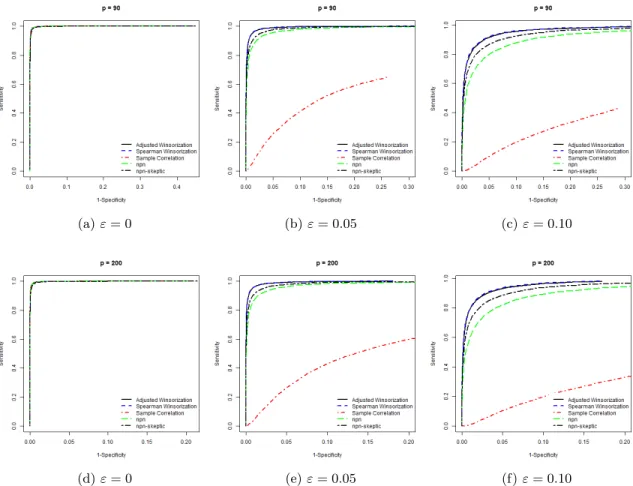
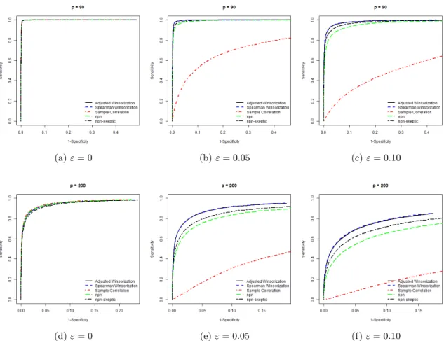
Figures2and 3illustrate the overall performance of different plug-in correlation estimates to robustly estimate the precision matrix under the first contamination mechanism for the full path of regularization parameters. For clean data, when the probability that a variable is contaminated is zero (i.e. ε= 0), the performance of the robust precision matrix estimates is similar to “Sample Correlation”. Under contamination, the performance of the different estimates change. Panel (b) and Panel (c) of Figures 2 and 3 show that under cellwise contamination (i.e. ε= 0.05 and ε= 0.10), “Sample Correlation” becomes very sensitive to the presence of cellwise outliers. Whenε= 0.05, we observe that the support recovery of “Adjusted Winsorization” and “Spearman Winsorization” performs slightly better than the robust estimates based on univariate outlier insensitive transformations. Whenε= 0.10 the precision matrix estimates based on bivarite winsorization significantly outperform the non-paranormal SKEPTIC proposed byLiu et al. (2012) and the winsorized normal-score nonparanormal fromLiu et al.(2009).
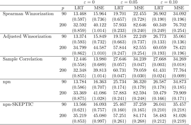
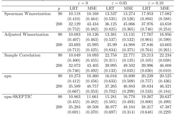
Tables1 and 2show the results for the numerical performance for the optimal regular-ization parameter under the first contamination mechanism when the precision matrix is specified as in the AR(1) Model and Erd¨os-R´enyi random graph, respectively. For clean data, the “Sample Correlation” sightly outperforms the robust plug-in estimators. The per-formance of the estimates based on bivariate winsorization is comparable with that of the empirical correlation matrix. Also, they slightly outperform the non-paranormal SKEPTIC and the winsorized normal-score nonparanormal estimator. When the probability that a variable contains outliers is positive, “Sample Correlation” performs very poorly in terms of efficiency on the precision matrix estimation. We observe that the robust estimators of the precision matrices have similar performance in terms of the expected likelihood ratio test and the mean squared error as the contamination increases. The similarity in their numerical performance is related with the fact that the BIC criteria selects models that contain a large number of false negatives.
Regarding the second contamination specification, simulation results can be sent upon request. Under this contamination mechanism the performance of the bivariate winsorized
(a)ε= 0 (b) ε= 0.05 (c)ε= 0.10
(d)ε= 0 (e)ε= 0.05 (f)ε= 0.10
Figure 2: AR(1)-Model Specification. ROC curves under the first contamination mechanism over 100 replications.
(a)ε= 0 (b) ε= 0.05 (c)ε= 0.10
(d)ε= 0 (e)ε= 0.05 (f)ε= 0.10
Figure 3: Erd¨os-R´enyi Specification. ROC curves under the first contamination mechanism over 100 replications.
estimates to recover the true GGM, for the AR(1) Model and Erd¨os-R´enyi random graph, confirms the insights of the first contamination mechanism.
As a summary, simulation results show that bivariate winsorization have better sup-port recovery performance in comparison with rank-based procedures. In general, both “Adjusted Winsorization” and “Spearman Winsorization” have satisfactory overall numer-ical performance properties. In terms of which method should be used, we observe that “Adjusted Winsorization” is slightly more efficient than “Spearman Winsorization” when the uncontaminated data is Gaussian distributed. This is due to the fact that the Spear-man’s rho is computed using univariate rank transformations, while adjusted winsorization operates directly on the data.
Table 1: AR(1)-Model Specification. Numerical performance under the first contamination mechanism over 100 replications with standard deviation in brackets.
ε= 0 ε= 0.05 ε= 0.10
p LRT MSE LRT MSE LRT MSE
Spearman Winzorization 90 13.468 15.964 19.701 22.455 26.902 34.092 (0.597) (0.736) (0.657) (0.728) (0.190) (0.196) 200 32.592 40.122 57.933 82.646 60.349 76.702 (0.859) (1.014) (0.233) (0.240) (0.249) (0.254) Adjusted Winsorization 90 13.374 15.849 19.518 22.249 26.773 35.061 (0.593) (0.732) (0.663) (0.737) (0.133) (0.136) 200 34.799 44.587 57.844 82.555 60.059 78.421 (0.862) (1.010) (0.247) (0.254) (0.193) (0.196) Sample Correlation 90 12.446 13.980 27.646 34.239 27.668 34.269 (0.558) (0.689) (0.057) (0.047) (0.003) (0.018) 200 32.348 39.813 60.731 79.059 61.431 77.764 (0.855) (1.014) (0.047) (0.030) (0.024) (0.009) npn 90 13.784 16.363 25.734 36.320 26.587 34.873 (0.586) (0.707) (0.174) (0.179) (0.178) (0.185) 200 33.369 41.086 57.883 82.594 59.479 79.909 (0.875) (1.028) (0.241) (0.248) (0.166) (0.171) npn-SKEPTIC 90 13.566 16.093 25.467 37.259 26.041 35.457 (0.621) (0.757) (0.160) (0.165) (0.210) (0.218) 200 35.219 45.080 57.251 84.174 58.483 81.026 (0.853) (0.997) (0.261) (0.268) (0.212) (0.219)
Table 2: Erd¨os-R´enyi Specification. Numerical performance under the first contamination mechanism over 100 replications with standard deviation in brackets.
ε= 0 ε= 0.05 ε= 0.10
p LRT MSE LRT MSE LRT MSE
Spearman Winzorization 90 10.118 10.168 13.537 13.274 17.953 17.082 (0.410) (0.464) (0.535) (0.526) (0.893) (0.588) 200 32.129 43.434 36.125 45.066 37.976 43.658 (0.752) (0.482) (0.825) (0.365) (0.746) (0.254) Adjusted Winsorization 90 10.083 10.126 13.381 13.131 17.767 16.956 (0.407) (0.463) (0.537) (0.532) (0.904) (0.599) 200 33.693 45.995 35.99 44.988 37.846 43.603 (0.712) (0.425) (0.834) (0.375) (0.764) (0.261) Sample Correlation 90 10.049 10.093 22.758 22.771 23.213 22.234 (0.400) (0.455) (0.311) (0.135) (0.105) (0.038) 200 32.073 43.405 39.995 49.502 39.996 46.808 (0.746) (0.492) (0.132) (0.035) (0.030) (0.010) npn 90 10.273 10.360 16.016 16.690 20.239 20.525 (0.412) (0.456) (0.633) (0.509) (0.757) (0.436) 200 35.589 48.757 37.265 46.883 38.834 46.321 (0.667) (0.353) (0.702) (0.299) (0.533) (0.184) npn-SKEPTIC 90 10.863 11.661 15.281 16.770 19.267 20.637 (0.455) (0.482) (0.585) (0.493) (0.800) (0.499) 200 35.283 48.508 36.977 48.104 38.317 47.387 (0.691) (0.370) (0.697) (0.314) (0.648) (0.229)
6
Robust Cancer Classification based on Gene Expression
Data
Microarrays experiments have being widely used to study the behavior of genes under various conditions. Microarrays raw data consist of image files and is subject to different preprocessing steps (Wu and Irizarry,2007). First, probe intensities are adjusted for optical noise or nonspecific binding. Then, the data is adjusted to remove systematic bias due to different experimental designs. This task is often called normalization. As a result, gene expression data is often subject to numerous sources of experimental and preprocessing errors (Daye et al., 2012) and it may contain outliers. Moreover, the violation of the Gaussian assumption can lead to bias in the recovery of the true undirected graph and
estimation of the precision matrix.
In this section we focus on the performance of robust precision matrices estimators for the classification of tumors using gene expression data. The different estimators are compared using two gene expression profile studies. For each study the data have being preprocessed, including image analysis of the microarray probe intensities, normalization and selection of differential expressed genes.
For an observed gene expression profilek we write the cellwise contamination model in the following form (seeAlqallaf et al.,2002):
Y(k)= (I−B)X(k)+BZ(k) fork= 1, . . . , n (6.1)
where Y(k) denotes the observed gene expression vector of p genes in mRNA sample k. The unobservable random vector of gene expression levelsX(k) is assumed to be Gaussian distributed,Z(k) ∈Rp is an arbitrary random vector and B is the contamination indicator matrix where P(B1 = 1) = . . . = P(B1 = 1) = ε (i.e. the probability of an outlier occurring in the each gene is the same). The mRNA samples belong to T known tumor classes, so a class label t(k) ∈ {1, . . . , T} can be predicted from the expression profiles
Y(k)= (Yi(k), . . . , Yp(k))T.
Based on the robust estimate of the precision matrix of the gene expression levels, we apply a linear discriminant analysis (LDA) to predict tumor classes. The different predictors are compared based on randomly splitting the data into training and testing sets. From the training set, we compute the robust center, scale and precision matrix estimates. For the test data we compute the linear discriminant score as follows
δt(Y(k)) =− 1 2log(det( ˆΩ))− 1 2d 2(Y(k),µˆ t,Ω) + logˆˆ πt, (6.2)
where ˆπt is the proportion of subjects in group t in the training set, ˆµt the within class
squared Mahalanobis distance. The classification rule is
ˆ
t(Y(k)) = argmaxδt(Y(k)) fort= 1, . . . , T. (6.3)
To perform model selection forλwe use 5-fold cross validation on the training data. Next, we analyze the performance of the bivariate winsorized precision matrix for the classification of tumors from gene expression datasets.
6.1 Analysis of Breast Cancer Data
We apply the procedure to evaluate gene expression profiling to breast cancer patients data to predict who may achieve pathological complete response (pCR). Using normalized gene expression data of patients in stages I-III of breast cancer data analyzed by Hess et al. (2006), we aim to predict response stated to neoadjuvant (preoperative) chemoterapy of patients with pathological complete response (pCR) and with residual disease (RD). The importance of analyzing the subject response to neoadjuvant (preoperative) chemoterapy, resides in the fact that complete eradication of all invasive cancer (i.e. pCR) is associated with long-term cancer free survival.
The data set consist of 22,283 gene expression levels of 133 subjects, with 34 pCR and 99 RD, respectively. We follow the analysis scheme proposed byFan et al. (2009) and Cai et al. (2011). The data is randomly split into the training and testing set, and we repeat this procedure 100 times. The testing set is formed by randomly selecting 5 pCR subjects and 16 RD subjects (approximately 1/6 subjects in each group). The remaining subjects form the training set. From the training set, a Wilcox singed-rank test is performed to select the 113 most significant genes.
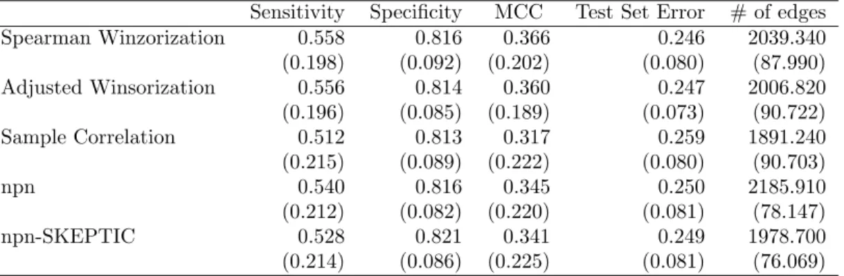
Table3displays the average classification performance and the number of missclassified pCR subjects (Test Set Error) for each precision matrix estimator. We observe that “Sample Correlation” has the worst performance in predicting the pCR subjects in comparison with the robust precision matrix estimates. The overall classification performance measure
by MCC criteria shows that “Adjusted Winsorization” outperforms the other procedures. From the results, we observe that the bivariate winsorized estimators improve over “npn” and “npn-SKEPTIC” in terms of the sensitivity and MCC, while all of them give similar specificity.
Table 3: Comparison of average pCR classification errors over 100 replications with standard deviation in brackets.
Sensitivity Specificity MCC Test Set Error # of edges Spearman Winzorization 0.558 0.816 0.366 0.246 2039.340 (0.198) (0.092) (0.202) (0.080) (87.990) Adjusted Winsorization 0.556 0.814 0.360 0.247 2006.820 (0.196) (0.085) (0.189) (0.073) (90.722) Sample Correlation 0.512 0.813 0.317 0.259 1891.240 (0.215) (0.089) (0.222) (0.080) (90.703) npn 0.540 0.816 0.345 0.250 2185.910 (0.212) (0.082) (0.220) (0.081) (78.147) npn-SKEPTIC 0.528 0.821 0.341 0.249 1978.700 (0.214) (0.086) (0.225) (0.081) (76.069)
6.2 Analysis of Leukemia Data
The Leukemia dataset comes from a study of gene expression in two types of acute leukemia: acute lymphoblastic leukemia (ALL) and acute myeloid leukemia (AML), and was described byGolub et al.(1999). It has been shown that is critical for determining the chemotherapy regime to obtain discriminating tumor tissues between ALL and AML. Gene expression levels were measured using Affymetrix high-density oligonucleotide arrays. The raw data set consists of 6,817 gene expression levels of 38 bone marrow samples (27 ALL and 11 AML). The data was preprocessed and reduced to a subset of 3,051 with the most differential gene expression values.
The preprocessed data is randomly split into the training and testing set, and we repeat this procedure 100 times. The training set is formed by randomly selecting 25 cases and the testing set by randomly selecting 13 tissue samples. The training set is formed by 18 ALL samples and 7 AML samples. From the training set, a Wilcox singed-rank test is performed
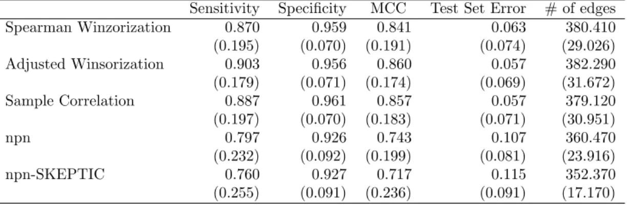
Table 4: Comparison of average leukemia classification errors over 100 replications with standard deviation in brackets.
Sensitivity Specificity MCC Test Set Error # of edges Spearman Winzorization 0.870 0.959 0.841 0.063 380.410 (0.195) (0.070) (0.191) (0.074) (29.026) Adjusted Winsorization 0.903 0.956 0.860 0.057 382.290 (0.179) (0.071) (0.174) (0.069) (31.672) Sample Correlation 0.887 0.961 0.857 0.057 379.120 (0.197) (0.070) (0.183) (0.071) (30.951) npn 0.797 0.926 0.743 0.107 360.470 (0.232) (0.092) (0.199) (0.081) (23.916) npn-SKEPTIC 0.760 0.927 0.717 0.115 352.370 (0.255) (0.091) (0.236) (0.091) (17.170)
to select the 50 most significant genes.
Table4displays the average classification performance and the number of missclassified tumor samples for each precision matrix estimator. The bivariate winsorized estimate based on adjusted winsorization has the better overall performance measure by MCC. We see that “Adjusted Winsorization” and “Spearman Winsorization” outperforms “npn” and “npn-SKEPTIC” in Sensitivity and MCC. In terms of Specificity all estimators have good performance in estimating false negatives. When we compare the rank-based procedures we observe that the winsorized normal-score nonparanormal estimator has better performance than the non-paranormal SKEPTIC estimator. This is due to the fact that when the contamination is low the “npn” is slightly more efficient than the nonparanormal SKEPTIC (see Liu et al.,2012).
7
Conclusions
In this article we have presented a method to robustly estimate a Gaussian Graphical model when the data contain outliers. Several authors, includingLiu et al. (2009) and Liu et al. (2012), have proposed robust estimators for the precision matrix in the high-dimensional setting. These methods are based on univariate outliers insensitive transformations to
achieve normality. These transformations guarantee the protection against outlier propa-gation. However, they are not robust under the presence of structural bivariate outliers which may lead to misleading graph support recovery. Our approach is able to handle structural bivariate outliers while protecting against outlier propagation.
We estimate a high-dimensional and sparse robust precision matrix by plugging a robust correlation matrix estimate into a constraint `1 log-determinant divergence. We estimate the robust correlation matrix applying robust affine equivariant methods to the bivari-ate data and compute robust pairwise weighted correlation estimbivari-ates, where the weights are computed by the Mahalanobis distance with respect to an affine equivariante robust correlation estimate. The proposed transformation applies a bivariate winsorization that shrinks observations to the border of a tolerance ellipse so that outlying observations are appropriately downweight to obtain a robust correlation estimate against two-dimensional structural outliers.
We analyze the analytic properties of the proposed bivariate winsorized pairwise scat-ter estimate and show that the rate of convergence is the same as the affine equivariant estimates used as a diagnostic tool to identify outlying observations. Furthermore, we show that if the initial robust affine equivariant correlation coefficient converges to the true correlation at the optimal parametric rate, then the bivariate winsorized precision matrix estimate achieves the optimal parametric rate in highdimensions.
Finally, we conducted extensive numerical simulations under different contamination settings to compare graph recovery performance of different robust estimators. We show that the proposed precision matrix estimate is robust against structural bivariate outliers and works well under the cellwise contamination model. The numerical simulations show that the bivariate winsorized transformation outperforms the existing rank-based methods when we aim to recover the support of Ω. Moreover, the proposed methods were then ap-plied to the classification of tumors using gene expression data and we obtained satisfactory and promising prediction results.
specific concentration bounds for the Spearman’s bivariate winsorization and the adjusted bivariate winsorization correlation coefficient. The performance of the bivariate winsorized estimate could also be studied under alternative precision matrix estimators such as CLIME (Cai et al., 2011), neighborhood selection with the lasso (Meinshausen and B¨uhlmann, 2006) and neighborhood Dantzig selector (Yuan, 2010). Also, we would like to establish the breakdown properties of the pairwise weighted correlation estimates under the cellwise contamination model. It would be important to determine the breakdown properties of the Graphical lasso when the bivariate winsorized correlation matrix is plugged into the`1 log-determinant divergence. Moreover, the proposed bivariate winsorized correlation coefficient could be used to perform robust correlation screening to deal with ultrahigh-dimensional data (see Li et al., 2012). Finally, it would be possible to study the bivariate outliers detection approach to estimate high-dimensional and sparse undirected graphs under more general elliptical distributions such as the multivariatet−distributions and nonparanormal models.
SUPPLEMENTARY MATERIAL
R script for Adjusted Winsorization R script cor.hub containing code to estimate the bivariate winsorized correlation matrix using adjusted winsorization describe in the article. (.R file)
R script for Spearman Winsorization R script cor.spearman containing code to esti-mate the bivariate winsorized correlation matrix using Spearman’s rho describe in the article. (.R file)
References
Alqallaf, F., S. V. Aelst, V. J. Yohai, and R. H. Zamar (2009). Propagation of outliers in multivariate data. The Annals of Statistics 37(1), 311–331.
Alqallaf, F. A., K. P. Konis, R. D. Martin, and R. H. Zamar (2002). Scalable robust covariance and correlation estimates for data mining. InProceedings of the eighth ACM SIGKDD international conference on Knowledge discovery and data mining, pp. 14–23. ACM.
Banerjee, O., L. El Ghaoui, and A. d’Aspremont (2008). Model selection through sparse maximum likelihood estimation for multivariate gaussian or binary data. The Journal of Machine Learning Research 9, 485–516.
Cai, T., W. Liu, and X. Luo (2011). A constrained `1 minimization approach to sparse precision matrix estimation. Journal of the American Statistical Association 106(494), 594–607.
Cerioli, A. (2010). Multivariate outlier detection with high-breakdown estimators. Journal of the American Statistical Association 105(489), 147–156.
Chen, J. and Z. Chen (2008). Extended bayesian information criteria for model selection with large model spaces. Biometrika 95(3), 759–771.
Danilov, M., V. J. Yohai, and R. H. Zamar (2012). Robust estimation of multivariate location and scatter in the presence of missing data. Journal of the American Statistical Association 107(499), 1178–1186.
Daye, Z. J., J. Chen, and H. Li (2012). High-dimensional heteroscedastic regression with an application to eQTL data analysis. Biometrics 68(1), 316–326.
Dempster, A. P. (1972). Covariance selection. Biometrics, 157–175.
Donoho, D. L. (1982). Breakdown properties of multivariate location estimators. Technical report, Technical report, Harvard University, Boston. URL http://www-stat. stanford. edu/˜ donoho/Reports/Oldies/BPMLE. pdf.
Edwards, D. (2000). Introduction to Graphical Modelling. Springer Science & Business Media.
El Karoui, N. (2008). Operator norm consistent estimation of large-dimensional sparse covariance matrices. The Annals of Statistics 36(6), 2717–2756.
Fan, J., Y. Feng, and Y. Wu (2009). Network exploration via the adaptive lasso and scad penalties. The Annals of Applied Statistics 3(2), 521–541.
Finegold, M. and M. Drton (2011). Robust graphical modeling of gene networks using classical and alternative t-distributions. The Annals of Applied Statistics, 1057–1080.
Friedman, J., T. Hastie, and R. Tibshirani (2008). Sparse inverse covariance estimation with the graphical lasso. Biostatistics 9(3), 432–441.
Golub, T. R., D. K. Slonim, P. Tamayo, C. Huard, M. Gaasenbeek, J. P. Mesirov, H. Coller, M. L. Loh, J. R. Downing, M. A. Caligiuri, et al. (1999). Molecular classification of cancer: class discovery and class prediction by gene expression monitoring. Science 286(5439), 531–537.
Hess, K. R., K. Anderson, W. F. Symmans, V. Valero, N. Ibrahim, J. A. Mejia, D. Booser, R. L. Theriault, A. U. Buzdar, P. J. Dempsey, et al. (2006). Pharmacogenomic predictor of sensitivity to preoperative chemotherapy with paclitaxel and fluorouracil, doxorubicin, and cyclophosphamide in breast cancer. Journal of Clinical Oncology 24(26), 4236–4244. Huber, P. J. (2011). Robust Statistics. Springer.
Huber, P. J. et al. (1964). Robust estimation of a location parameter. The Annals of Mathematical Statistics 35(1), 73–101.
Kendall, M. and J. Gibbons (1990). Rank correlation methods. A Charles Griffin Book. E. Arnold.
Khan, J. A., S. Van Aelst, and R. H. Zamar (2007). Robust linear model selection based on least angle regression. Journal of the American Statistical Association 102(480), 1289–1299.
Khan, M. J. A. (2006). Robust Linear Model Selection for High-dimensional Datasets. Ph. D. thesis, University of British Columbia.
Kruskal, W. H. (1958). Ordinal measures of association.Journal of the American Statistical Association 53(284), 814–861.
Lam, C. and J. Fan (2009). Sparsistency and rates of convergence in large covariance matrix estimation. Annals of Statistics 37(6B), 4254–4278.
Lauritzen, S. L. (1996). Graphical Models. Oxford University Press.
Ledoit, O. and M. Wolf (2004). A well-conditioned estimator for large-dimensional covari-ance matrices. Journal of Multivariate Analysis 88(2), 365–411.
Li, G., H. Peng, J. Zhang, and L. Zhu (2012). Robust rank correlation based screening. The Annals of Statistics 40(3), 1846–1877.
Liu, H., F. Han, M. Yuan, J. Lafferty, and L. Wasserman (2012). High-dimensional semi-parametric gaussian copula graphical models. The Annals of Statistics 40(4), 2293–2326. Liu, H., J. Lafferty, and L. Wasserman (2009). The nonparanormal: Semiparametric estimation of high dimensional undirected graphs. Journal of Machine Learning Re-search 10(Oct), 2295–2328.
Liu, H. and L. Wang (2012). Tiger: A tuning-insensitive approach for optimally estimating gaussian graphical models. arXiv preprint arXiv:1209.2437.
Liu, L., D. M. Hawkins, S. Ghosh, and S. S. Young (2003). Robust singular value de-composition analysis of microarray data. Proceedings of the National Academy of Sci-ences 100(23), 13167–13172.
Loh, P.-L. and X. L. Tan (2015). High-dimensional robust precision matrix estimation: Cellwise corruption under epsilon-contamination. arXiv preprint arXiv:1509.07229. Lopuha¨a, H. P. (1999). Asymptotics of reweighted estimators of multivariate location and
scatter. Annals of Statistics 27(5), 1638–1665.
Maronna, R. A. (1976, 01). Robustm-estimators of multivariate location and scatter. The Annals of Statistics 4(1), 51–67.
Meinshausen, N. and P. B¨uhlmann (2006). High-dimensional graphs and variable selection with the lasso. The Annals of Statistics 34(3), 1436–1462.
¨
Ollerer, V. and C. Croux (2015). Robust high-dimensional precision matrix estimation. In Modern Nonparametric, Robust and Multivariate Methods, pp. 325–350. Springer. Peng, J., P. Wang, N. Zhou, and J. Zhu (2009). Partial correlation estimation by joint sparse
regression models. Journal of the American Statistical Association 104(486), 735–746. Ravikumar, P., G. Raskutti, M. J. Wainwright, and B. Yu (2008). Model selection in
gaus-sian graphical models: High-dimensional consistency of l1-regularized MLE. In NIPS, pp. 1329–1336.
Ravikumar, P., M. J. Wainwright, G. Raskutti, B. Yu, et al. (2011). High-dimensional covariance estimation by minimizing 1-penalized log-determinant divergence. Electronic Journal of Statistics 5, 935–980.
Ren, Z., T. Sun, C.-H. Zhang, H. H. Zhou, et al. (2015). Asymptotic normality and opti-malities in estimation of large gaussian graphical models. The Annals of Statistics 43(3), 991–1026.
Rothman, A. J., P. J. Bickel, E. Levina, J. Zhu, et al. (2008). Sparse permutation invariant covariance estimation. Electronic Journal of Statistics 2, 494–515.
Rousseeuw, P. J. (1984). Least Median of Squar