Management
Jian Ren
A dissertation submitted in partial fulfillment of the requirements for the degree of
Doctor of Philosophy of the
University of London.
Department of Computer Science University College London
This thesis investigates the application of Search Based Software Engineering (SBSE) approach in the field of Software Project Management (SPM). With SBSE ap-proaches, a pool of candidate solutions to an SPM problem is automatically gen-erated and gradually evolved to be increasingly more desirable. The thesis is mo-tivated by the observation from industrial practice that it is much more helpful to the project manager to provide insightful knowledge than exact solutions. We inves-tigate whether SBSE approaches can aid the project managers in decision making by not only providing them with desirable solutions, but also illustrating insightful “what-if” scenarios during the phases of project initiation, planning and enactment. SBSE techniques can automatically “evolve” solutions to software requirement elicitation, project staffing and scheduling problems. However, the current state-of-the-art computer-aided software project management tools remain limited in several aspects. First, software requirement engineering is plagued by problems associated with unreliable estimates. The estimations made early are assumed to be accurate, but the projects are estimated and executed in an environment filled with uncertain-ties that may lead to delay or disruptions. Second, software project scheduling and staffing are two closely related problems that have been studied separately by most published research in the field of computer aided software project management, but software project managers are usually confronted with the complex trade-off and correlations of scheduling and staffing. Last, full attendance of required staff is usu-ally assumed after the staff have been assigned to the project, but the execution of a project is subject to staff absences because of sickness and turnover, for example. This thesis makes the following main contributions: (1) Introducing an au-tomated SBSE approach to Sensitivity Analysis for requirement elicitation, which helps to achieve more accurate estimations by directing extra estimation effort to-wards those error-sensitive requirements and budgets. (2) Demonstrating that Co-evolutionary approaches can simultaneously co-evolve solutions for both work pack-age sequencing and project team sizing. The proposed approach to these two inter-related problems yields better results than random and single-population evolution-ary algorithms. (3) Presenting co-evolutionevolution-ary approaches that can guide the project manager to anticipate and ameliorate the impact of staff absence. (4) The investiga-tions of seven sets of real world data on software requirement and software project plans reveal general insights as well as exceptions of our approach in practise. (5) The establishment of a tool that implements the above concepts. These contribu-tions support the thesis that automated SBSE tools can be beneficial to solution generation, and most importantly, insightful knowledge for decision making in the practise of software project management.
First and foremost, I would like to thank my supervisorProf. Mark Harman. He is the best supervisor one could ever expect for.
I would also like to thank my second supervisorDr. Jens Krinke, my early PhD
mentorProf. Zheng Li, and my previous external advisorProf. Anthony Finkelstein.
I am grateful to the following external personnel for their generous help and
valuable expertises on some specific topics: Prof. Xin Yaoat University of
Birming-ham,Prof. Massimiliano Di Pentaat University of Sannio,Prof. Giuliano Antoniol
at ´Ecole Polytechnique de Montr´eal,Prof. Francisco Palomo Lozano and Prof.
In-maculada Medina Bulo at University of C´adiz, Prof. G¨unther Ruhe at University
of Calgary, and Prof. Filomena Ferrucci and Dr. Federica Sarro at University of
Salerno.
My greatest gratitude is reserved for all my fellow colleagues in CREST (Centre for Research on Evolution, Search and Testing) whose advice, help and support are
always available at those critical moments, especially to Dr. William Langdon,Dr.
David Clark,Dr. Afshin Mansouri,Dr. Shin Yoo, andDr. Yuanyuan Zhang. Finally
and very importantly, I would like to thank the CREST admin,Ms. Lena Hierl, for
the kindest and most professional administrative support.
This thesis is dedicated to my inspiring grandparents, my beloved parents, and my supportive family and friends.
Chapters 4 and 5 of this thesis have been published as:
• J. Ren, S. Yoo, M. Harman and J. Krinke, Search Based Data Sensitivity
Analysis Applied to Requirement Engineering,Proceedings of the 11th Genetic
and Evolutionary Computation Conference (GECCO 2009), pages 1681-1688.
Cited by 171.
• J. Ren, M. Harman and M. Di Penta, Cooperative Co-evolutionary
Optimiza-tion of Software Project Staff Assignments and Job Scheduling,Proceedings of
the 3rd International Symposium of Search Based Software Engineering (SS-BSE 2011), pages 127-141. Cited by 91.
The following papers have been published or submitted during the course of this PhD programme, although they do not form a part of this thesis:
• F. Ferrucci, M. Harman, J. Ren and F. Sarro, Not Going to Take this Anymore:
Multi-Objective Overtime Planning for Software Engineering Projects,
Pro-ceedings of the 35th International Conference on Software Engineering (ICSE 2013), accepted on 20 November 2012.
• M. Harman, J. Krinke, I. M. Bulo, F. P. Lozano, J. Ren and S. Yoo, Empirical
Evaluation of Exact Sensitivity Analysis for the Next Release Problem,ACM
Transactions on Software Engineering and Methodology, under revision.
• A. Finkelstein, M. Harman, S. A. Mansouri, J. Ren and Y. Zhang, A Search
Based Approach to Fairness Analysis in Requirement Assignments to Aid
Ne-gotiation, Mediation and Decision Making,Requirements Engineering Journal,
14(4):231-245, December 2009. Cited by 241.
• J. Ren, Y. Zhang, A. Finkelstein, M. Harman and S. A. Mansouri, . “Fairness
Analysis” in Requirements Assignments,Proceedings of the 16th International
Requirements Engineering Conference (RE’08), pages 115-124. Cited by 281.
1
Abstract . . . 2 Acknowledgements . . . 3 List of Publications . . . 4 List of Figures . . . 10 List of Tables . . . 15 List of Algorithms . . . 17 1 Introduction 18 1.1 Search-based Software Engineering . . . 18
1.2 Software Project Management . . . 20
1.3 Contributions of this Work . . . 21
1.4 Research Methodology . . . 22
1.5 Layout of the Thesis . . . 23
2 Literature Review 26 2.1 Software Project Management . . . 26
2.1.1 Software Life Cycle Process Models . . . 27
2.1.2 Challenges in Software Project Management . . . 29
2.1.3 Industry Standards and Practices for PM . . . 31
2.1.4 Risk Management in Software Development . . . 32
2.2 Software Cost Estimation . . . 35
2.3 Sensitivity Analysis . . . 37
2.4 Evolutionary Computation . . . 40
2.4.1 Evolutionary Algorithm . . . 42
2.4.1.2 Genetic Programming . . . 42
2.4.1.3 Evolutionary Strategy . . . 42
2.4.1.4 Evolutionary Programming . . . 43
2.4.1.5 Co–evolutionary Genetic Algorithm . . . 43
2.4.2 Competitive Co–evolutionary Algorithm . . . 43
2.4.3 Cooperative Co-evolutionary Algorithm . . . 44
2.5 Search Based Software Engineering . . . 44
2.5.1 Origins and Applications . . . 44
2.5.2 Software Project Management with Meta-heuristics . . . 45
2.5.2.1 Project Scheduling Problem with Meta-heuristics . 46 2.5.2.2 Project Resource Allocation with Meta-heuristics . 47 3 Industrial Data for Evaluation 50 3.1 Industrial Requirement Data . . . 50
3.2 Industrial Project Plan Data . . . 51
3.2.1 Industrial Contexts of Real Software Projects . . . 51
3.2.2 Features and Characteristics of Projects and Visualisations . 53 3.3 Limitations of Data Usage . . . 54
4 Sensitivity Analysis on Cost Estimation of Requirements Selection 61 4.1 Introduction . . . 61
4.2 Background . . . 63
4.2.1 Single-objective Next Release Problem . . . 63
4.2.2 Multi-objective Next Release Problem . . . 65
4.3 Sensitivity Analysis in NRP . . . 65 4.4 SA Experimental Set Up . . . 68 4.4.1 Greedy Algorithm . . . 69 4.4.2 NSGA-II . . . 70 4.4.3 Requirement Data . . . 70 4.4.4 Evaluation . . . 71 4.4.5 Research Questions . . . 71
4.5.1 Result From Single-Objective Formulation . . . 72
4.5.2 Result From Multi-Objective Formulation . . . 75
4.5.3 Statistical Analysis . . . 79
4.5.4 Answers to the Research Questions . . . 81
4.6 Related work . . . 82
4.7 Summary . . . 82
5 Cooperative Co-evolutionary Job Sequencing and Team Sizing 84 5.1 Introduction . . . 84
5.2 Problem Statement and Definitions . . . 85
5.2.1 Ordering/Sequence of Work Packages . . . 86
5.2.2 Staff Assignments to Teams . . . 87
5.2.3 Scheduling Simulation . . . 87
5.3 Optimisation Method: Cooperative Co-evolutionary Algorithm . . . 88
5.3.1 Solution Representations and Genetic Operators . . . 88
5.3.2 Initial Populations . . . 89
5.3.3 Termination Condition . . . 89
5.4 Empirical Study . . . 90
5.5 Empirical Study Results . . . 92
5.5.1 Analysis of the Cooperative Co-Evolutionary Progress . . . . 92
5.5.2 Results on Effectiveness . . . 97
5.5.3 Results on Efficiency . . . 99
5.5.4 Threats to Validity . . . 100
5.6 Related Work . . . 101
5.7 Summary . . . 102
6 Co-evolutionary Project Planning Optimisation under Staff Ab-sence 104 6.1 Introduction . . . 104
6.1.1 Research Questions . . . 107
6.2 Problem Statement . . . 107
6.2.2 Staff Availability Calendar(STCAL) . . . 108
6.3 Co-evolution . . . 109
6.3.1 Genetic Representations . . . 109
6.3.1.1 Array of WP’s IDs representing Work Package Or-dering . . . 109
6.3.1.2 Boolean matrix representingStaff Availability Calendar109 6.3.2 Genetic Operators . . . 110
6.3.2.1 Order Crossover on WPO . . . 110
6.3.2.2 Mutation on WPO . . . 110
6.3.2.3 Dependency and Duplication Verification on “new-born” WPO . . . 111
6.3.2.4 Uniform Crossover on Staff Availability Calendar. . 111
6.3.2.5 Mutation onStaff Availability Calendar . . . 111
6.3.3 Fitness Evaluation and Selection of Candidate Solutions . . . 112
6.3.3.1 Scheduling Simulation . . . 112
6.3.4 Overall Co-evolution Procedure . . . 115
6.4 Empirical Study . . . 116
6.4.1 Parameter Setting . . . 116
6.4.2 Four Configurations of Co-evolutionary Optimisation . . . 118
6.5 Results Analysis . . . 119
6.5.1 Running Time . . . 120
6.5.2 Average External Assessment of the Solutions Found . . . 122
6.5.3 Trend of Improvement on Solutions in the Process of Searching 125 6.5.4 Detailed Case Analysis on Configuration BWBS . . . 126
6.5.5 Answers to the Research Questions and Proposals to the PM 131 6.6 Measuring the Absence Rate . . . 133
6.7 Summary . . . 134
7 Conclusions and Future Works 135 7.1 Summary of Contributions . . . 136
7.3 Closing Remark . . . 138
Appendices 139
A Results of Co-evolutionary Project Management Optimisation on
Four Real–world Projects 139
A.1 Competitive Searching for Better WPOs and Worse STCALs . . . . 139
A.2 Competitive Searching for Worse WPOs and Better STCALs . . . . 144
A.3 Cooperative Searching for Worse WPOs and Worse STCALs . . . . 149
A.4 Cooperative Searching for Better WPOs and Better STCALs . . . . 154
1.1 GA crossover for reproduction . . . 19
1.2 Simplified flow chart of a genetic algorithm . . . 19
2.1 Breakdown of topics covered in the Software Engineering Management
KA. Figure adapted from [Abran et al., 2004]. . . 27
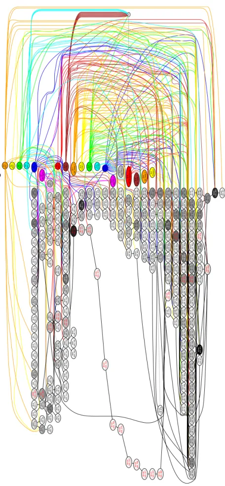
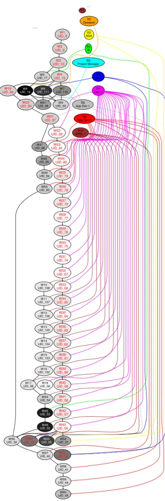
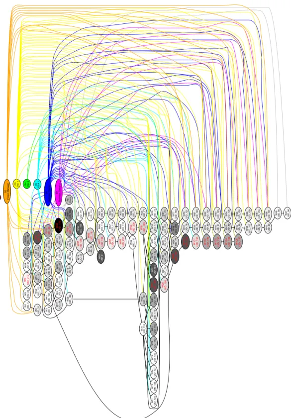
3.1 Work Package Dependency Graph of Project B. It shows the work
packages, the normalised efforts (degree of greyness), dependency
re-lationship among WPs (black lines), and the critical path (WPs that
marked with red tags: W[id] and UID [uid]). . . 56
3.2 Work Package Dependency Graph and Resource Allocation Graph of
Project C. In addition, it shows the resources (coloured ellipsis), and
the corresponding WPs require such resources (coloured lines). . . . 57
3.3 Work Package Dependency Graph and Resource Allocation Graph of
Project D . . . 58
3.4 Work Package Dependency Graph and Resource Allocation Graph of
Project E . . . 59
3.5 Work Package Dependency Graph and Resource Allocation Graph of
Project F . . . 60
4.1 Sensitivity Analysis Flow Chart . . . 66
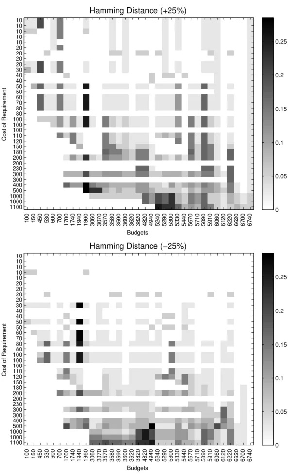
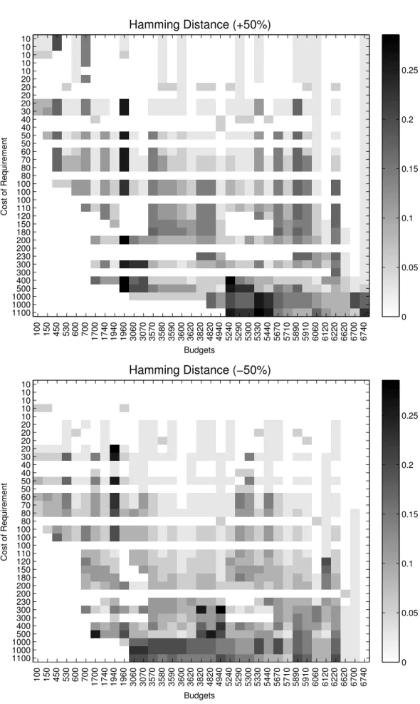
4.2 Hamming distance from the original solution to the solution obtained
by the greedy algorithm with PIAC value of±25%. . . 73
4.3 Hamming distance from the original solution to the solution obtained
4.4 Euclidean distance between original estimated Pareto-front and actual
Pareto-front by different PIAC values. . . 76
4.5 Boxplots of Euclidean distances between Pareto-fronts for different
costs of requirements . . . 77
4.6 Boxplots of Euclidean distances between Pareto-fronts for different
PIAC values . . . 78
5.1 WPO Chromosome: The gray area is the representation of the
so-lutions for the ordering for distributing a set of l work packages. A
solution is represented by a string of length l, each gene
correspond-ing to the distributcorrespond-ing order of the WPs and the alleles, drawn from
{1, ..., l}, representing an individual WP. . . 86
5.2 TC Chromosome: The gray area is the representation of the solutions
for Team Construction or the assignments of a set ofnstaff to a set of
m teams. A solution is represented by a string of lengthn, with each
gene corresponding to a staff and the alleles, drawn from {1, ..., m},
representing assignment of the staff. . . 87
5.3 Crossover for Team Construction solutions: Single Point Crossover . 89
5.4 Mutation on Work Package Ordering solution: Randomly Swap WPs’
Positions . . . 89
5.5 Projects A: Boxplots of completion times for all solutions found by
different CCEAs configurations . . . 93
5.6 Projects B: Boxplots of completion times for all solutions found by
different CCEAs configurations . . . 94
5.7 Projects C: Boxplots of completion times for all solutions found by
different CCEAs configurations . . . 95
5.8 Projects D: Boxplots of completion times for all solutions found by
different CCEAs configurations . . . 96
5.9 Boxplots of all the best solutions found in 30 runs of the three CCEA
configurations, and in random search runs . . . 98
6.1 Sickness absence as a proportion of working time. Figure adapted
from [Black, 2008] . . . 106
6.2 WPO Chromosome: The gray area is the representation of one
spe-cific ordering for distributing a set of lwork packages. As shown the
solution is represented by a string of length l, each gene
correspond-ing to the distributcorrespond-ing order of the WPs and the alleles, drawn from
{1, ..., l}, representing one WP’s ID. . . 109
6.3 The representation of Staff Availability Calendarwith “1” indicating
the day a member of staff is not available . . . 110
6.4 WPO Crossover: Order Crossover . . . 110
6.5 WPO Mutation: Randomly Swap WPs’ Positions . . . 110
6.6 Uniform Crossover on Staff Availability Calendar: offspring inherit
availabilities of one specific member of staff as for the whole period of the project (a whole row on the chromosome) from either of the
parents with equal probability. . . 112
6.7 Mutation on Staff Availability Calendar: for each member of staff,
the positions of a ’1’ and a random ’0’ are swapped with a defined
probability. . . 112
6.8 Scheduling simulation with Work Package Orderingand Staff
Avail-ability Calendar. The scheduling simulator takes one WPO solution and one STCAL solution as its inputs. The simulation result illus-trates the process of a corresponding project being executed, such as:
project completion time,staff-to-WP allocation. . . 113
6.10 External fitness of solutions by Configuration BWBS on Project C. The solutions for two species are plotted separately in two side-by-side sub-figures, with the WPOs on the left and STCALs on the right. The sub-figures are arranged in three rows according to their levels of the absence rate equal to 0.001, 0.1, and 0.25 respectively. The finish time of the entire population is plotted for each generation along the co-evolutionary process. A solid line on the boxes is the mean value of each generation. The duration of executing the critical path for each project is plotted accordingly as a dashed line near the bottom
of each sub-figure. . . 127
6.11 External fitness of solutions by Configuration BWBS on Project D . 128 6.12 External fitness of solutions by Configuration BWBS on Project E . 129 6.13 External fitness of solutions by Configuration BWBS on Project F . 130 A.1 C – BWWS – Internal Fitness . . . 140
A.2 C – BWWS – External Fitness . . . 140
A.3 D – BWWS – Internal Fitness . . . 141
A.4 D – BWWS – External Fitness . . . 141
A.5 E – BWWS – Internal Fitness . . . 142
A.6 E – BWWS – External Fitness . . . 142
A.7 F – BWWS – Internal Fitness . . . 143
A.8 F – BWWS – External Fitness . . . 143
A.9 C – WWBS – Internal Fitness . . . 145
A.10 C – WWBS – External Fitness . . . 145
A.11 D – WWBS – Internal Fitness . . . 146
A.12 D – WWBS – External Fitness . . . 146
A.13 E – WWBS – Internal Fitness . . . 147
A.14 E – WWBS – External Fitness . . . 147
A.15 F – WWBS – Internal Fitness . . . 148
A.16 F – WWBS – Internal Fitness . . . 148
A.18 C – WWWS – External Fitness . . . 150
A.19 D – WWWS – Internal Fitness . . . 151
A.20 D – WWWS – External Fitness . . . 151
A.21 E – WWWS – Internal Fitness . . . 152
A.22 E – WWWS – External Fitness . . . 152
A.23 F – WWWS – Internal Fitness . . . 153
A.24 F – WWWS – External Fitness . . . 153
A.25 C – BWBS – Internal Fitness . . . 155
A.26 C – BWBS – External Fitness . . . 155
A.27 D – BWBS – Internal Fitness . . . 156
A.28 D – BWBS – External Fitness . . . 156
A.29 E – BWBS – Internal Fitness . . . 157
A.30 E – BWBS – External Fitness . . . 157
A.31 F – BWBS – Internal Fitness . . . 158
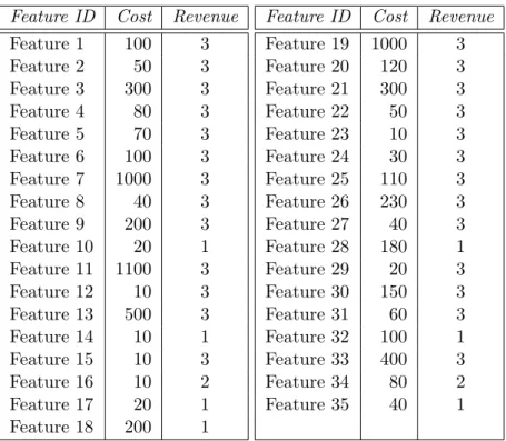
3.1 Data of thirty five software features for a future model of a mobile
phone from Motorola Inc.. Adapted from [Baker et al., 2006]. . . 51
3.2 Features of all six software projects . . . 53
4.1 Spearman’s rank correlation coefficient between PICA value and
Eu-clidean distance. For all requirements, the observed ρ values are
sta-tistically significant at the confidence level of 95%. . . 80
4.2 Spearman’s rank correlation coefficient between cost and Euclidean
distance. For all PICA values, the observedρ values are statistically
significant at the confidence level of 95%. . . 80
5.1 Three sets of configurations for CCEA each of which requires the same
total number of evaluations before it is terminated. F represents the
number of evaluation required in one generation, and it is fixed for all
configurations in this empirical study. . . 90
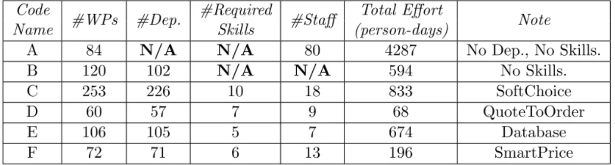
5.2 Characteristics of the four industrial projects . . . 91
5.3 Wilcoxon Rank Sum Test (unpaired) test adjusted p-values for the
6.1 The table shows the average fitness of the solutions found by algo-rithms in terms of their externally assessed project finish time (Days). This reveals the quality of the solutions found in the last generation of the co-evolutionary process. The maximum and minimum values in each row are highlighted in bold font. Extrema tend to be found in cooperative search, especially in the solutions of WPO in cooperative search. In competitive search, optimisation on WPO dominates the competition on complex projects (C and E), whilst optimisation on
STCAL dominates the competition on simpler projects (D and F). . 121
6.2 The Spearman’s rank correlation coefficient table indicates the trend
in the improvements of average external fitness values of the entire population as the co-evolutionary progress proceeds over generations. The values highlighted in bold font indicate the cases in which there
is no statistically significant overall trend of improvement. . . 124
1 Greedy Algorithm . . . 69
2 NSGA-II Algorithm . . . 70
Introduction
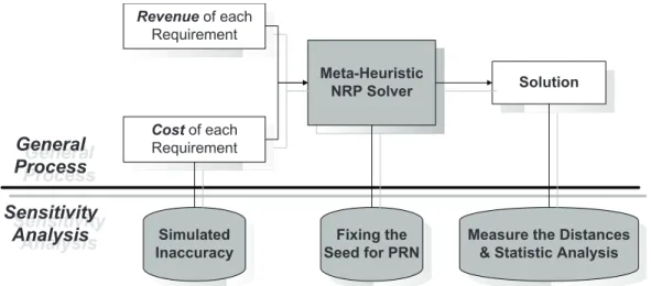
This thesis addresses the study of applying the Search Based Software Engineering (SBSE) approach to several software project management problems. In this chapter, introductions of the SBSE as well as the problems to be tackled are presented, the major contributions of this work are highlighted, and the layout of this thesis is presented.
1.1
Search-based Software Engineering
As a set of techniques to apply meta-heuristic algorithms to software engineering problems, Search Based Software Engineering (SBSE) [Harman and Jones, 2001] is becoming an increasingly popular paradigm for the study and implementation of solving software engineering problems that are highly complex and dynamic [Harman et al., 2012]. It works by using search-based algorithms to automatically generate solutions, and “evolving” them gradually to optimal or near optimal solutions.
Genetic Algorithms (GAs) [Holland, 1992] have been identified as one of the most widely used search-based algorithms for SBSE [Harman, 2007]. Genetic algo-rithms maintain one population of individual solutions to a specific problem. Each individual solution is represented as a chromosome that carries its genetic informa-tion (DNA) which defines how such an individual plans to solve the corresponding problem. Depending on how well one individual solves the underlining problem, a value is assigned to represent such individual’s “fitness”. Naturally, GA repeatedly chooses those “fitter” solutions to reproduce (Figure 1.1) new individuals. The new individuals then compete with their parent populations as well as their siblings. The “fitter” individuals survive, form the population in the current generation, and
re-produce the next generation. When this iteration of selection and reproduction ends, the individuals in the last generation are expected to be the optimal or near optimal solutions. The sequence of these operations is given in Figure 1.2.
Parent A: 1 2 3 4 5 6 7 Offspring: 1 2 3 6 4 7 5 4 4 OO OO OO Parent B: 6 2 3 1 4 7 5
Figure 1.1: GA crossover for reproduction
Initial Population Fittness Evaluation Selection Reproduction Mutation Stop? end F T
Co-evolutionary genetic algorithm [Hillis, 1990, Potter and Jong, 1994] is very important extension of standard GA that allows the optimisation process to “evolve” more than one population of solutions, among which they are inter-related with those in the other population. According to how the fitness of one individual might affect the fitness evaluation of other individuals, the relationship across co-evolving population can be competitive [Hillis, 1990] or cooperative [Potter and Jong, 1994].
1.2
Software Project Management
Software project scheduling and staffing problems have been tackled by heuristic algorithm by Chang et al. [Chang et al., 2001,Chang et al., 2008,Ge and Chang, 2006, Chang et al., 1998], Alba et al. [Alba and Chicano, 2005, Alba and Chicano, 2007], and many other researchers [Gueorguiev et al., 2009, Antoniol et al., 2005, Alvarez-Valdes et al., 2006, Chan et al., 1996, Hindi et al., 2002]. In fact, GA has been widely studied in tackling software project management as a project scheduling problem. However, the current state-of-the-art research demonstrate a lack of flexibility to effectively cope with the dynamic of modern software projects, such as, changing staff during the project is not allowed in the models.
From all those previous studies on software project scheduling and staffing, we have known how to optimise the schedule of a software project under ideal condi-tions such as accurate estimacondi-tions given on: 1) accurate estimacondi-tions on the effort of each individual work packages, and 2) comprehensive knowledge of resources, e.g.: provision for individual project staff.
However, in the practices of software project engineering management, the project team is assembled and staff is allocated to work packages according to a given “optimised” project schedule. This given schedule can no longer be considered to be “optimised” once the staff information become fully available, because the hired staff’s skills, efficiencies and availabilities are often guaranteed to be different from the ones that were used to optimise the schedule.
Therefore, there is a need to simultaneously optimise these two closely related problems together, and we decided to investigate the co-evolutionary algorithm’s ad-vantage that enables us to study the impact of the interconnections between multiple
subproblems.
In fact, unlike the work in this thesis, none of the previous work on project scheduling and staffing has used a co-evolutionary optimisation approach. More importantly, our co-evolutionary model allows us to investigate uncertainties caused by unplanned changes such as changing requirements and staff absence which can not be easily coped with by traditional standard GA.
1.3
Contributions of this Work
This thesis makes a main contribution of demonstrating that advanced SBSE tech-niques can be beneficial in solving software project management problems at the stages of project initiation (Chapter 4), planning (Chapter 5) and enactment (Chap-ter 6). The contributions of this thesis are elaborated as follows::
1. It presents an automated Sensitivity Analysis approach to identify sensitive requirements and budgets with respect to inaccurate cost estimation. The approach is based on SBSE for both single-and-multi-objective Next Release Problem formulations.
2. It introduces Cooperative Co-Evolutionary Algorithms to the software project
staffing and scheduling problems for the first time. A Cooperative
Co-evolutionary Algorithm is able to outperform random search and single popu-lation genetic algorithm on software project staffing and scheduling problems. 3. It presents empirical studies of four real world software projects planning data that demonstrate co-evolutionary optimisation techniques that can, not only find solutions to compensate the impact of staff absence during the project execution, but also provide various insightful knowledge that can aid project manager in making better and safer decisions.
4. It presents the establishment of a tool calledAmphisbaena 1 (AMPHI- Search
Based manAgEmeNt Approach). Currently, Amphisbaena provides intuitive
1
Amphisbaenanoun [am(p)-f@s-"b¯e-n@] from: merriam-webster.com Definition: a serpent in classical mythology having a head at each end and capable of moving in either direction
Origin: Latin, from Greek ‘amphisbaina’, from ‘amphis’ on both sides (from ‘amphi’ around) + ‘bainein’ to walk, go
visualisations for sensitivity analysis on requirement estimation, and it also provides solutions and insights of staffing and scheduling via the automated
analysing process that is operated directly on the MicrosoftR Project Plan
(*.mpp) file.
In summary, the thesis proposes the following three main steps in software project management process: 1) the SBSE sensitive analysis to help on achieving more accurate estimations during requirement selection, 2) the cooperative co-evolutionary approach to help on attaining more effective project staffing and scheduling, and 3) the co-evolutionary approach to help on compensate the impact of staff absence. These contributions support the thesis that automated SBSE assistance can provide both solutions and insightful knowledge to a software project management problems across the entire software development life cycle from the project’s initiation, through planing to its enactment.
1.4
Research Methodology
This research adopts the quantitative research method to systematically and empir-ically investigate three software project management problems. In particular, this thesis tackles the problems which cause software project managers: 1) suffering from unreliable estimations during requirement selection, 2) not being able to co-optimise staffing and scheduling when they are planning the project, and 3) being difficult to management staff absence during the enactment of a project.
In essence, the empirical experimentations are designed in answering the follow-ing three sets of research questions: 1) How does SBSE sensitivity analysis help in understanding the correlation of the key factors (i.e., cost and inaccuracy) and the revenue of the final solution, and how to understand the exceptions to the general trends? 2) Can cooperative co-evolutionary algorithm outperforms random search and conventional genetic algorithm in co-optimising the staffing and scheduling prob-lems, and how effective and efficient? 3) How do co-evolutionary optimisation tech-niques reveal and compensate the impact of staff absence?
The research questions are answered by the empirical studies based on the quan-titative data and statistical analysis on the result. The first set of quanquan-titative
re-search questions mainly ask for the significance of the correlation between two pairs
of variables: {cost and impact} and {inaccuracy and impact}. Positive correlation
assumptions are statistically tested against both synthetic and real-world require-ment data. Spearman’s rank correlation coefficient shows that strong positive corre-lations exist at the confidence level of 95%. The second set of quantitative research questions focus on the comparisons of the performance of random algorithm, conven-tional evolutionary algorithm and the cooperative co-evolutionary algorithms. The empirical studies on different algorithms are conducted on four real world software projects. The Wilcoxon Rank Sum Test on the results found that the cooperative co-evolutionary algorithm performs better than the conventional 1-population
evo-lutionary algorithm with great statistical significance (p ≤1.28E−06). The third
set of quantitative research questions mainly ask to identify the configurations of co-evolutionary algorithm that are able to find more extreme solutions than the others under the combined influence of staff absence and project complexity.
During the course of answering the research questions, a set of automated tools simulating project enactment are developed. Seven sets of real world requirement and project planning data are used to perform empirical experiments. Statistical tools are utilised to analyse the correlations between variables and the comparison of different optimisation techniques.
1.5
Layout of the Thesis
This thesis is organised as follows:
Chapter 2 - Literature Reviewsummarises the literature in the fields of software
project management, techniques for sensitivity analysis, evolutionary optimisation, search based software engineering and its applications in software project manage-ment.
Chapter 3 - Industrial Data for Evaluationdescribes the real world data sets
used for the empirical studies in this thesis. The chapter begins by describing a set of software requirements from Motorola Inc.. The cost and revenue of each requirement are listed. The chapter then introduces each of the six sets of real world software
projects’ plans by: describing the industrial context, summarising the key features, and visualising the key information.
Chapter 4 - Sensitivity Analysis on Cost Estimation of Requirements
Selectionpresents an approach to sensitivity analysis in a requirement selection
problem. The approach uses search based software engineering to aid the decision maker to explore sensitivity of the cost estimates of requirements for the Next Release Problem (NRP). The chapter presents both single- and multi-objective formulation of NRP with empirical sensitivity analysis on synthetic and real-world data. Then the chapter moves on to the analysis of the empirical study in which the some intuitive assumptions are confirmed. A heat-map style visualisation tool is presented to reveal those counter-intuitive exceptions which require careful consideration.
Chapter 5 - Cooperative Co-evolutionary Job Sequencing and Team
Siz-ingintroduces an new approach to search based software project management based
on Cooperative Co-evolution. The approach aims to “co-optimise” both work pack-age scheduling and developers’ team staffing problems simultaneously by applying co-operative co-evolutionary techniques to achieve early overall finish time. The chapter first introduces the models of the problems to apply the cooperative co-evolutionary approach in generating, reproducing, and eliciting desirable solutions. The solution evaluation is based on the simulation of executing such a project plan which consists of two solutions to each of the two problems. The chapter then presents the results of the empirical study using real world projects data from four different software companies. The cooperative co-evolution is demonstrated to be more efficient and effective than single population evolution and random search.
Chapter 6 - Co-evolutionary Project Planning Optimisation under Staff
Absenceextends the work in Chapter 5 to consider how to fully utilise advantage of
co-evolutionary project planning technique to help the project manager to mitigate possible impact of staff absence. The key to analysing the impact of staff absence is first to be able to distinguish the staff by their skill, and then to simulate the absence at different stages of a project. The chapter extends the design of the problem model of staffing, as introduced in Chapter 5, to allow the representation of staff’s absence
in a staff availability calendar. The scheduler simulating the execution of project plan is completely redesigned to accommodate the new job assignment rules that are associated with the skills. This chapter then presents four new configurations of co-evolutionary optimisation techniques and their empirical studies on four real world software project data. The result demonstrates the co-evolutionary software project planning technique is able to provide lower and upper bound of current project’s finish time, identify the dominating problem during the execution of current project, and provide useful insights on the correlations among staff absence rate, the delay caused, and the complexity of a project.
Chapter 7 - Conclusionsconcludes the thesis with a summary of its major
Literature Review
2.1
Software Project Management
Project management is a broad subject, and all of its subtopics cannot be covered in this thesis. Therefore, the thesis is focused on Software Project Management, including cost and scheduling estimation, risk management, and staff assignment optimisation.
In general, a project can be defined as a series of activities that are conducted to achieve one or more specific objectives at a specified cost and within a specified time [Hughes et al., 2004]. Essentially, a management method is a set of processes used to run a project in a controlled and, therefore, predictable fashion. In the con-text of software engineering, we focus on projects that develop new software, and the management activities including: planning, coordinating, measuring, monitor-ing, controllmonitor-ing, and reportmonitor-ing, which collectively ensure that the development and maintenance of the software is systematic, disciplined, and quantified [Abran et al., 2004, IEEE610.12-1990, 1990].
The Software Engineering Coordinating Committee, which is sponsored by the IEEE Computer Society, has developed an all–inclusive collection of knowledge within the profession of software engineering that is known as the Software En-gineering Body of Knowledge (SWEBOK) [Abran et al., 2004]. SWEBOK suggests the 10 Knowledge Areas (KAs) that form the classification of the scheme of the field, i.e., Software Requirements, Software Design, Software Construction, Software Testing, Software Maintenance, Software Configuration Management, Software En-gineering Management, Software EnEn-gineering Process, Software EnEn-gineering Tools
and Methods, and Software Quality.
With regard to the software project management, SWEBOK specifically in-cludes a breakdown that allows the Software Engineering Management KA to be viewed as an organisational process. As shown in Figure 2.1, the primary basis for the top-level breakdown is the process of managing a software engineering project. The software project management process is addressed in its first five subareas, and software engineering measurement is addressed in the last sub–area.
Figure 2.1: Breakdown of topics covered in the Software Engineering Management KA. Figure adapted from [Abran et al., 2004].
2.1.1 Software Life Cycle Process Models
Waterfall Model:The Waterfall model is the oldest and most well known software
development process in sequential phases and suggests that the current phase should be completed and checked for accuracy before proceeding to the next phase. By using the Waterfall model, the software project manager expects each task to be completed properly the first time it is done. However, for most software projects, the developers’ knowledge and understanding of the information related to the project become clearer as the processing proceeds. Therefore, if some important details are discovered that were unknown at the beginning of the project, the Waterfall
developing model requires the process to be restarted. So, the Waterfall model
works best for projects for which the required information is known and static, the objectives of project are clearly defined, and there is a very low probability of any surprise.
Spiral Model:The Spiral model, which was developed by Boehm in 1988 [Boehm,
1988], was designed to overcome the Waterfall model’s major weaknesses. In the Spiral model, a project starts with the development of a small set of requirements to guide the developers’ effects through the whole process. Then, in each of the fol-lowing iterations, the development team add additional requirements to the product based on the experience gained from the previous iterations and any new, available external knowledge that may be available about the product. This iterative approach results in a more flexible development process to that is able to adapt to changing requirements. It also reduces the risks by providing opportunities for the objectives to be refined and for the risks to be reassessed at the end of each iteration.
V–Model:The V–model was first introduced for use in Germany’s federal IT
projects [Sommerville, 1992]. It pays special attention to improving the commu-nication between the developer and the customer by associating the analysis and development phases with the corresponding testing processes. This approach allows the provisions of guidelines so that both developers and customers can contribute cooperatively to the project.
Agile Methods:New software is integrated seamlessly into people’s every day lives,
and software development is no longer viewed as a technically demanding activity that only serious scientists can do. Quite often, the software engineers begin coding when only a small fraction of the requirements are clearly defined and well before the
overall design structure of the software has been finalised. Since even the customers might not have a clear idea of what all their needs are at the beginning of the software development process, the early finalisation of the overall structure of software that is being developed is very difficult. Most importantly, the requirements often change during the course of the development process. Therefore, it is unrealistic to enforce an exact “plan” for the software when its development has just begun.
In a traditional “Plan Driven” development process, an attempt is made to plan all the requirements and changes upfront. At the beginning of the process, efforts are made to anticipate any changes in the requirements that may be needed, and, subsequently, the goal of the following management activities is to try to ensure that the project is developed according to plan, hoping that nothing goes wrong.
Agile “spirit” guides the project management to attempt to achieve “working software” in very short periods of an incremental development cycle. The “plan” is to develop the software along with its overall structure until the customer is satisfied or the resources are used up. The goal is the development of functional software that satisfies the customer, and Agile methods attempt to achieve this by emphasising the role of the day-to-day input of customers in keeping the process moving in the right direction. In general, the software system and the requirements are developed gradually as the development activities take place.
In February 2001, the Agile Manifesto [Beck et al., 2001] was published and the Agile Alliance was found to promote Agile methods including SCRUM and Extreme Programming. SCRUM [Schwaber and Beedle, 2001] is one of the earliest Agile soft-ware project management methods while Extreme Programming [Beck and Andres, 2004] is one of the most widely used software development methods [Boehm, 2006].
2.1.2 Challenges in Software Project Management
The Software Engineering Management KA [Abran et al., 2004] addresses the man-agement of software engineering project and the measurement of software. It also identifies some of the key aspects that are specific to a software project and that
complicate the effective management of such projects. Harmanet al. [Harman et al.,
2009b] identified a number of unresolved challenges in software project planning, including: lack of robustness in planning, poor estimates and lack of appropriate
integration of the various processes. These problems that are specific to software project management are summarised below in items 1 through 6 and the remaining unresolved challenges are summarised in item 7 through 9:
1. Lack of appreciation for the complexity inherent in Software Engineering, par-ticularly in relation to the impact of changing requirements.
2. Changing requirements that might be generated by the clients (customers) or by the software engineering processes themselves.
3. Iterative Developing Process: software is often built in an iterative process rather than a sequence of closed tasks.
4. Software engineering necessarily incorporates aspects of creativity and disci-pline, and maintaining an appropriate balance between the two is often difficult. 5. The degree of novelty and complexity of software is often extremely high. 6. There is a rapid rate of change in the underlying technology.
7. Often, the importance of robustness in planning is overlooked; it may be more important to develop plans that are robust and can accommodate changes than to develop plans that lead to early completion.
8. The unreliability of price and schedule estimates is problem that constantly plagues software project development activities— [Jø rgensen and Shepperd, 2007].
9. Appropriate integration of the process steps is often overlooked: software project management is not an activity that can be optimised in isolation. It is necessary to develop techniques to integrate management activities with other activities, such as design, testing, maintenance, or even with other engineering, such as requirement engineering.
Herroelen [Herroelen, 2005] provided a list of the 12 reasons that are often cited for the escalation of project costs and schedules. In examining that list, it is apparent that none of them is related to the technology used in the project; rather, they are
more related to human factors in the project management process. Keil [Keil et al., 2003] gathered data for an information system based on a survey of 376 information system audit and control professionals in the U.S. Bryde [Bryde, 2003] conducted an empirical study of project management practices in projects in the UK. The tools that are used in project management are project tracking, time analysis, cost analysis, and resource analysis. Herroelen suggested that “proper use of project management software may well not be considered the most important driving force behind project success.”
2.1.3 Industry Standards and Practices for PM
Major project management practices in the real–world are listed below:
Critical Path Method (CPM) [Kelley Jr and Walker, 1959]: Developed by
DuPont Corporation, CPM is a scheduling algorithm to analyse the ordering of work packages.
Program Evaluation Review Technique (PERT) [Malcolm et al., 1959]:
In-vented by US Department of Defense for a US Navy Project, PERT is a method to calculate the total completion time of a project by analysing the completion time of each task involved in the project.
Work Breakdown Structure (WBS) [Jø rgensen, 2004b, Tausworthe, 1980]:
Also invented by US Department of Defense, WBS is a hierarchical tree structure that contains all the subtasks that need to be done to complete the whole project.
SCRUM [Schwaber and Beedle, 2001]: Scrum is an agile software development
model based on multiple small teams working in an intensive and interdependent manner.
A Guide to the Project Management Body of Knowledge (PMBOK
Guide) [PMI, 2004]: Published by Project Management Institute, PMBOK is an
standard of accepted project management information and practices. The latest (4th) edition was released in 2008.
Earned Value Management (EVM): EVM is a set of techniques for measuring
Total Cost Management (TCM): TCM is a process for applying the skills and knowledge of cost engineering.
PRojects IN Controlled Environments (PRINCE, PRINCE2): It provides
a method for managing projects within a clearly defined framework.
Theory of Constraints (TOC), Critical Chain Project Management
(CCPM): CCPM is developed from TOC. It aims to analyse constraints on the
project and manage the resources to keep the whole project on schedule.
2.1.4 Risk Management in Software Development
Boehm [Boehm, 1991, Boehm and Ross, 1989] introduced the concept of Software Risk Management into the field of Software Engineering in the 1980s. He summarised four types of sources of software risk addressed by risk management techniques:
• Potential software errors
• Overruns of budget and schedule
• Not satisfying functionality or performance requirements
• Developing a product which is hard to modify or use in other situations
Boehm offered a six–step risk management process to assess and control these sources of risk. The six steps are grouped into two categories called assessment and control as follows: • Risk Assessment 1. Risk Identification 2. Risk Analysis 3. Risk Prioritisation • Risk Control
4. Risk Management Planning 5. Risk Resolution
6. Risk Monitoring
With regards to the risk caused by software errors, an example of the Risk Reduction Leverage calculation is given in Boehm’s paper [Boehm and Ross, 1989] to confirm that the investments in risk management with verification and validation (V&V) in the early stages of a software project have a higher pay-off ratio than investments that are made in testing later on. For the sake of easy identification,
the most common risk items on a software project, i.e., a checklist of the “Top 10 Primary Sources of Risk on Software Projects,” are summarised based on their survey of a number of experienced project managers. He identified the difficulty of making accurate estimations of the possibility of the occurrence of a risk and the associated loss identified by the checklist. This leads to an inaccurate risk assessment and, consequently, to poor risk control. Boehm mentioned some techniques to improve the estimation of the probability of the occurrence of a risk. For simplicity, the risk probabilities and losses are assessed on a relative scale of 0 to 10.
Fairley [Fairley, 1994] provided a design of the process that was more practical than Boehm’s. He created a seven-step process for risk management was based on several years of work with numerous organisations to identify and overcome risk factors in software projects:
1. Identify risk factors
2. Assess risk probabilities and effects on the project 3. Develop strategies to mitigate identified risks 4. Monitor risk factors
5. Invoke a contingency plan 6. Manage the crisis
7. Recover from the crisis
An example of risk management for a project to implement a telecommunications protocol for a network gateway was proposed to demonstrate his mathematical model of the assessment of risk probabilities and effects. However, unlike Boehm, he sug-gested no additional tools or methods.
In the practice of Software Project Risk Management, different project man-agers tend to focus on different aspects of risk analysis. Moynihan [Moynihan, 1997] confirmed this even with his survey of only 14 experienced application systems de-velopers in Ireland on the topic of “How experienced project managers assess risk.” More importantly, he analysed the risk factors summarised from the survey and
compared them with those risk factors identified in the software project manage-ment literature, such as Barki’s Risk Variable [Barki et al., 1993] and SEI Risk Question [Carr et al., 1993]. The analysis suggested that it is unrealistic to build a single, universal risk taxonomy for use by all software development projects, which means a universal “checklist” for software project risk management does not exist. Project risk management has different taxonomies within different project contexts, just as we might expect.
Before a meaningful risk management plan can be developed, risks must be identified in advance. Despite the different aspects of the risk management process, both Boehm and Fairley started their risk management process by Risk Factors Identification. However, since a universal “checklist” does not exist and experts’ risk management is highly dependent on their experience, researchers tend to seek out and use the tools or models that will help the experts analyse risks that have specific characteristics to determine their impacts on the project.
Keil et al. [Keil et al., 1998] proposed a risk categorisation framework for iden-tifying software project risk based on two dimensions, i.e., perceived level of control, and perceived relative importance of the risk. They assembled three panels of more than 40 software project managers from all over the world to rank the importance of a common set of 11 risk factors. The project managers had little or no input concern-ing the risk factors that were considered to be the most important. Subsequently, the study results suggested that the software project manager should expand her or his risk assessment to include the factors over which project managers have relatively little control, such as risks relative to customer mandates, which were identified among the most important risks but which were missing entirely from Boehm’s top 10 checklist of possible risk sources [Boehm and Ross, 1989].
With the help of their risk framework, Wallace and Keil subsequently investi-gated [Wallace and Keil, 2004] how different types of risk influence project outcomes by collecting and analysing input from more than 500 software project managers. The study showed that managing the risks related to a project’s execution, scope, and requirements is critical. Project management almost always requires tradeoffs to deal with the triple constraints of scope, cost, and schedule.
A recent empirical study by Odzaly et al. [Odzaly and Des Greer, 2009] indicated that a sample of 18 experienced software project managers had good awareness of risk management but a low usage of the tools required to perform risk management on projects. The authors also sought to develop an agent-based, automatic tool to bypass the perception that the risk management process is costly, which has been confirmed as a major barrier that prevents or reduces its application in software project management practice. Gueorguiev et al. [Gueorguiev et al., 2009] introduced a search-based approach to identify and quantitatively analyse the risk associated with project scheduling.
To summarise, many research and standardisation efforts have been attempted in the field of risk analysis for software project management, but, in practice, prac-titioners still tend to avoid using the recommended approaches based on the facts that 1) a set of “standard” risk management processes is generally unacceptable to software project managers and 2) it is costly to do so.
Automated or semi–automated tools have become important in advancing the practice of risk management to a new level. As indicated in Section 2.5 of this review, Search Based Software Engineering (SBSE) techniques are the ideal tool to automate the risk analysis process in software project management. Within the context of SBSE, project managers have the choice of defining the objectives that they think are more important for successful completion of the current project or using the SBSE tool to determine the optimal or near–optimal candidate solutions.
2.2
Software Cost Estimation
Software cost estimation is critical for the success of software projects management. Depending on whether the final step of the estimation is a mechanical quantification step, such as a formula, there are two ways to estimate costs during the software project planning phase, as indicated in Expert Judgment–Based Estimations and Formal Model–Based Methods [Jø rgensen et al., 2009].
According to an extensive review of software estimation models and techniques conducted by Boehm in 2000 [Boehm et al., 2000], these methods can be
mathemat-ical models to measure and calculate estimates for the development efforts, such as COCOMO and COCOMO II [Boehm, 1984, Boehm et al., 1995], SLIM
[Put-nam and Myers, 1992], and Check Point [Jones, 1997]; 2)expertise–based techniques
that help practitioners provide estimates based on their knowledge and experiences, such as the Delphi method [Boehm, 1984, Helmer et al., 1966] and Work Breakdown
Structure-based methods [Jø rgensen, 2004b,Tausworthe, 1980]; 3)learning–oriented
techniques that perform the estimation by “learning” from previous experience. The “learning” process can be done manually, such as the Case Based Reasoning (CBR) approach [Aamodt and Plaza, 1994], or automatically, such as the Machine
Learn-ing approach [Goldberg, 1989]; 4) dynamics–based models developed by Jay
For-rester [ForFor-rester and Wright, 1961] that acknowledge the change of software project
efforts or cost over the duration of the development of the system; 5) regression–
based modelsthat include the “Standard” regression – Ordinary Least Squares (OLS) method [Griffiths et al., 1993] and the “Robust” regression (e.g., Least–squares of In-verted balanced Relative errors (LIRS)) [Miyazaki et al., 1994], which is an improved version of OLS that alleviates the common problem of outliers in observed software
engineering data and 6)composite methods that combine two or more techniques to
accommodate the needs of different project situations.
Researchers have a strong inclination to combining their expert judgment with the results of formal methods for developing estimates of software development ef-forts. In a recent debate [Jø rgensen et al., 2009] with Boehm on “which is better for software development estimation: formal models or expert judgement?” Jorgensen claimed that the most important advantage of the judgment-based method is that the experts’ highly specific knowledge is difficult to include in the formal models. Boehm argued that parametric models contain a significant amount of information on which factors cause software costs to change and by how much. He also argued that organisations are performing extensive sensitivity, risk, and trade–off analyses to narrow the cone of uncertainty, but these analyses are complex and time consuming. On the other hand, industrial surveys have indicated that formal models-based methods are seldom used by software practitioners, mainly because of the high cost of implementing formal models and the insignificant benefits that result from their
use [Yang et al., 2008a]. Due to the people–centric nature of software engineering, an accurate cost estimation system has yet to be developed and remains as one of the unachieved challenges in Software Engineering [Shepperd, 2007].
In addition to the nature of the “high cost” and inaccuracies of estimation techniques, project uncertainties are also of considerable importance [Jø rgensen, 2004a]. Large differences between estimated and actual effort do not necessarily indicate poor estimation skills. While it is important to analyse the degree of the uncertainties of the estimate, it might be more helpful for the decision maker to gain insight into the effects caused by the uncertainties during the cost estimation phase [Gueorguiev et al., 2009, Harman et al., 2009a].
2.3
Sensitivity Analysis
As discussed in Sections 2.1.4 and 2.2 concerning risk analysis and cost estimation, it was indicated that, due to variables that are unpredictable, software engineers are not able to predict accurately actual risks or cost. While various models and procedures have been developed in attempts to achieve more accurate predictions of the parameters, some researchers have been attempting to prevent failures in projects with a slightly different approach; they have tried to identify the parameters that are more sensitive to inaccurate estimations.
Sensitivity Analysis (SA) refers to “the determination of the contribution of individual, uncertain analysis inputs to the uncertainty in analysis results” [Helton et al., 2006]. Usually, when a system becomes increasingly complex, it becomes increasingly difficult or even impossible to derive and summarise the relationship be-tween the inputs and outputs of the system using a mathematical model. Sensitivity analysis is a set of techniques used to analyse the relationship between the inputs and outputs of a complex system based on the input parameters and the observed outputs produced by the system. Generally, sensitivity analysis is used to identify the input parameters that most significantly influence the system’s outputs.
Applications of SA are widely found in the literature for various areas, such as chemical kinetics [Sandu et al., 2003], physical science [Newman et al., 1999], en-vironmental modelling [Hamby, 1994], telecommunications engineering [Racu et al.,
2005], and financial analysis [Levine and Renelt, 1992]. A few typical usages of SA techniques have been selected and classified into the following categories for experi-mentations of evolutionary computation:
One–At–a–Time (OAT) methods [Saltelli et al., 2000] are the simplest of the various methods, and they are also referred to as Local Sensitivity Analysis [Saltelli et al., 2008] or Nominal Range Sensitivity Analysis [Christopher Frey and Patil, 2002]. Conceptually, these methods vary one parameter at a time repeatedly, while all of the other parameters are maintained at their fixed, baseline values. The major drawback of OAT methods is that the interactions between parameters are not taken into account in the analysis. Therefore, results from OAT methods and global sen-sitivity analyses can be contradictory [Thogmartin, 2010]. Several possible ways for correcting OAT methods have been proposed recently by Saltelli et al., including full factorial design methods, the regression effects method, and the elementary effects method, which they note can be used “...at no extra cost.” [Saltelli and Annoni, 2010].
Factorial Design (FD) [Box et al., 1978] overcomes the major drawback of the OAT methods by selecting a given number of samples for each parameter and running the model for all combinations of the samples. In this case, the interactions between parameters are considered. However, it is not feasible to use this method to perform SA on a model with a large number of parameters because of the tremendous number of runs required. In 2006, Helton et al. [Helton et al., 2006] conducted a comprehen-sive survey of uncertainty and sensitivity analysis techniques using sampling-based (e.g., Monte Carlo (MC)) methods.
The Elementary Effects (EE) [Morris, 1991] Method was first introduced by Morris in 1991 to accommodate the needs for SA from models that are deterministic and complicated with a large number of input parameters, which makes “classical”
SA methods impractical. The elementary effect of theith input xi is defined below
for a given set ofk inputs whose values are denoted by vectorX :
where y is the output of the model, and ∆ is the simulated “error” on xi. (Note:
X here is not the basic line.) Suppose r sample values forxi are selected; for each
sample value, we have an elementary effect value for this particular input. Then the mean and standard deviation are calculated for the elementary effects for this input as follows: µi = 1 r r X 1 di(X) (2.2) σi= v u u t 1 r−1 r X 1 {di(X)−µi}2 (2.3)
A large measure of mean value,µ, indicatesxi has a large “overall” influence, while
a high value of standard deviation,σ, indicates non-linear effects or thatxi interacts
with other inputs. Obviously, low values of both variables indicates that input is non-influential. EE methods are considered to be a very good compromise between accuracy and efficiency, especially for sensitivity analysis of large models [Campo-longo and Braddock, 1999]. Aiming at improving Morris’ strategy on randomly sampling the input space, Campolongo et al. recently enhanced the strategy to gain a better spread of the input domain without increasing the number of model executions needed [Campolongo et al., 2007].
Box and Wilson (1951) first developed the Response Surface Methodology (RSM) for determining optimum conditions in a chemical investigation [Box and Wil-son, 1951]. Since that time, RSM has been of value for many other fields [Bucher, 1990, Carley et al., 2004, Hill and Hunter, 1966, Isukapalli et al., 2000, Khuri and Mukhopadhyay, 2010]. The underlying idea of RSM is to try to reduce the num-ber of computational experiments necessary to explore the input/output relationship space. It provides a way to develop and/or simplify the model itself by rigorously choosing a few points on the response surface to effectively represent all the possi-ble points. Then, the sensitivity analysis can be determined by investigation of the response surface, i.e., inspection of the functional form of the response surface.
In summary, OAT methods and FD can be considered as “brute force” strategies for tuning the input parameters to determine the features of the output results, while the EE method attempts to sample the parameters with care. Furthermore, other
methods, such as RSM, simplify the model and subsequently prioritise the input parameters. Practitioners are more likely to use the combinations of these methods mentioned above [Saltelli, 2004,Saltelli, 2005,Saltelli et al., 2004,Saltelli et al., 2008]. It is worth mentioning that Uncertainty Analysis (UA) and Sensitivity Analysis are often coupled in practice [Saltelli and Annoni, 2010]. However, the objectives of UA and SA are different. Uncertainty analysis refers to “the determination of the uncertainty in analysis results that derives from uncertainty in analysis inputs” [Hel-ton et al., 2006] and answers the question, “How uncertain is this inference?” On the other hand, sensitivity analysis aims to answer the question, “Where is this uncertainty coming from?” [Saltelli and Annoni, 2010].
2.4
Evolutionary Computation
The inspiration for using Evolutionary Computation (EC) to solve engineering or science problems came from the model of Darwinian evolution and biological the-ory [Darwin, 1859]. EC uses the Darwinian concepts of evolution and the principles of natural selection to automate the process of solving problems. Possible solutions for an underlying problem are considered as “individuals”. The evaluation of each individual is calculated by the fitness function. Higher fitness values indicate bet-ter quality solutions for the given problem. Each individual is encoded with the “chromosomes” on which the genetic operations (i.e., crossover and mutation) are conducted. Finally, the candidate solutions with higher fitness values survive dur-ing the process of “selection” and produce their “offsprdur-ing” by means of crossover and mutation. The new population, which consists of the candidate solutions that survived and their offspring, is called a new generation. As such, under the force of evolutionary pressure, the whole population evolves better solutions gradually over generations. A brief introduction to each step of this evolutionary process is provided below.
Representation:The representation of solutions reflects how the designer
under-stands the problem domain and the solution domain. There are two representations that are most frequently used, i.e., individuals could represent the solution for a real world optimisation problem as a binary string (GA) or individuals could represent
the solution in the form of a vector of real numbers (ES). In both cases, the evalu-ation process is based on extracting informevalu-ation from these representevalu-ations, which will be given to an objective function to calculate the fitness.
Initialisation:Random is most frequently used for initialisation. Because the first
generation of individuals is generated randomly, all the individuals of the first gen-eration are distributed randomly in the search space, providing diverse information about the search space. It is the easiest way to initially randomise the population, because the knowledge of search space is not necessary in the procedure of random initialisation.
Evaluation:The evaluation process is to determine the fitness value of the
individ-uals. The objective function(s) used to calculate the fitness value represent(s) the ultimate goal of the optimisation, which should be clearly defined by the designer. The algorithm should conduct the evaluation methods, which could then be used to direct the algorithm to identify the “fittest” solution(s), subject to constraints of resources.
Selection:The selection procedure is based mainly (but not necessarily fully) on
the fitness value of each individual. The individuals with higher fitness values will be more likely to survive and produce offspring. On the other hand, the individuals with less fitness values could also be selected when they have, for instance, high potentials to contribute to the diversity of the population and produce high-fitness-value offspring. The ultimate goal of selection is to maintain a population of high fitness individuals and provide an optimal set of solutions.
Genetic Operators:Mutation and Crossover (Recombination) are the two methods
used to generate offspring from the current population with the hope of producing better individuals in the offspring. The process of mutation is to alter a small portion of an individual’s chromosome, hoping to introduce more fit genes. The process of crossover (recombination) involves mixing the genes from two selected individuals (chromosomes), hoping to combine the best genes to produce stronger offspring.
Termination:The process of evolution could be endless iterations of “survival of
the fittest”. The designer must decide when to terminate the iterations and achieve the final survivals. This decision could be made based on the evaluation of the
population (how good the population is) or based on the constraint of the resources that run the algorithms, i.e., the amounts of time and money that can be spent on it.
2.4.1 Evolutionary Algorithm
The Evolutionary Algorithm (EA) is a sub-set of EC. There are two prominent fea-tures that distinguish EAs from other search algorithms: 1) EAs are all population-based and 2) there are communications and information exchange among individuals or between populations [Yao, 1996]. Due to the different configuration in the im-plementations, four major EAs have been developed under the same concepts of evolution that were aforementioned.
2.4.1.1 Genetic Algorithm
The Genetic Algorithm (GA) refers to a model introduced and investigated by John Holland in 1975 [Holland, 1992]. GA is one of the most popular types of EAs. The representation of the individuals in a GA is normally in the form of strings of numbers. It has been used mostly to evolve solutions in the parameterised problem domain [Goldberg, 1989, Kicinger et al., 2005].
2.4.1.2 Genetic Programming
Genetic Programming (GP) [Koza and Poli, 2005, Koza, 1992] has a tree structure to represent individual candidate solutions, while it is attempting to evolve actual computer programs. With the tree-structure chromosome representation, a complex mathematical model or a program can be expressed well, and, then, the genetic operations can perform the evolution process accordingly. GP has been used to evolve actual computer programs for solving a number of computational tasks [Langdon and Poli, 2002].
2.4.1.3 Evolutionary Strategy
The Evolutionary Strategy (ES) approach was first introduced by
Rechen-berg [RechenRechen-berg, 1964] and Schwefel [Schwefel, 1965]. One genetic operator,
Crossover (recombination), is less commonly used in ES. On the other hand, mu-tation operator on each individual is guided by parameters that evolves along with individuals themselves. In such cases, the genetic operation process is able to adapt
to the given problem automatically.
2.4.1.4 Evolutionary Programming
Evolutionary Programming (EP) was pioneered by L. Fogel, A. Owens, and M. Walsh in 1966 [Fogel et al., 1966] and recently refined by D. Fogel [Fogel, 1991]. There is no fixed representation or structure to distinguish EP from the other EAs. Therefore, researchers found it hard to distinguish EP from the other EAs on the theoretical level [Weise, 2009]. Detailed elaborations of the mechanism and comparisons of ES,
GA, and EP can be found in the literature [B¨ack and Schwefel, 1993].
2.4.1.5 Co–evolutionary Genetic Algorithm
Co-evolutionary computation research is another very important extension of stan-dard GA. Axelord was one of the first to introduce ideas of modelling the behaviour of natural co-evolution in game theory [Axelrod and Dion, 1988, Axelrod and Hamil-ton, 1981]. Hills [Hillis, 1990], Husbands and Mill [Husbands and Mill, 1991], and Paredis [Paredis, 1994] were the earliest researchers to implement Co-evolutionary GA (CGA). Hills used two populations to evolve the sorting networks and test cases simultaneously. Husbands and Mill applied two populations to evolve two fractions of solutions independently for a job-shop scheduling problem. Paredis evolved the constraints and solutions in two different populations for an “n-queen” problem.
In the context of evolutionary computation, co-evolution refers to evolving more than one independent population. The feature that distinguishes the co-evolutionary GA from the standard GA is that the evaluation of individuals is based on the interactions with other individuals instead of being conducted alone. Depending on the nature of these interactions, CGAs are further classified into two types, i.e., Competitive CGA and Cooperative CGA.
2.4.2 Competitive Co–evolutionary Algorithm
Competitive CGA maintains different candidate solutions in multiple populations that simulate competing relationships, such as predator-pray. For example, in Hills’ early implementation [Hillis, 1990], the objective of one population is to evolve in-creasingly better sorting networks, while the objective of the other population is to evolve increasingly difficult test cases for the sorting network. In such a case,
![Figure 2.1: Breakdown of topics covered in the Software Engineering Management KA. Figure adapted from [Abran et al., 2004].](https://thumb-us.123doks.com/thumbv2/123dok_us/1114921.2648402/27.892.169.745.378.883/figure-breakdown-covered-software-engineering-management-figure-adapted.webp)