Simple measurement models for complex working-memory tasks

Strickhofstrasse 39 CH-8057 Zurich www.zora.uzh.ch

Year: 2019

Simple measurement models for complex working-memory tasks Oberauer, Klaus ; Lewandowsky, Stephan

Abstract: We introduce a framework for simple measurement models for working memory, and apply it to complex-span and memory-updating tasks. Memory Measurement Models (M3) use the frequency distribution across response categories to measure continuous memory strength along 2 dimensions: Mem-ory for individual elements, potentially relying on persistent activation of unified representations, and memory for relations, relying on temporary bindings. Experiment 1 provides evidence for the validity of the parameters measuring these two dimensions of strength. The effects of experimental manipulations on these 2 dimensions can be captured by additional model parameters that reflect hypothetical pro-cesses affecting memory. Across five further experiments we illustrate how M3 can be used to measure 3 such processes: The continued strengthening of memory representations during the retention interval (extended encoding), the dampening of encoding of irrelevant information (filtering), and the removal of irrelevant information from memory. In one experiment we compare young and old adults on complex-span tasks and working memory updating. In both paradigms, old adults showed impaired memory for relations but no impairment in memory for individual elements. There was partial evidence for age differences in extended encoding and removal; there were no age differences in filtering. We suggest that M3 offer a computationally efficient approach to identifying memory processes. (PsycINFO Database Record (c) 2019 APA, all rights reserved).

DOI: https://doi.org/10.1037/rev0000159

Posted at the Zurich Open Repository and Archive, University of Zurich ZORA URL: https://doi.org/10.5167/uzh-175049

Journal Article Submitted Version

Originally published at:

Oberauer, Klaus; Lewandowsky, Stephan (2019). Simple measurement models for complex working-memory tasks. Psychological Review, 126(6):880-932.

Simple Measurement Models for Complex Working-Memory Tasks

Klaus Oberauer University of Zurich

Stephan Lewandowsky

University of Bristol and University of Western Australia

Preprint posted on PsyArXiv: osf.io/vkhmu

The research reported in this article was supported by funding from the University Research Priority Program "Dynamics of Healthy Aging" at the University of Zurich, as well as from the Swiss National Science Foundation (SNSF, grants number 100014_149193 and 100014_143333) to the first author, and a fellowship from the Royal Society to the second author. We are grateful to Danielle Pessach for assistance with collecting the data.

Correspondence should be addressed to: Klaus Oberauer, University of Zurich, Department of Psychology – Cognitive Psychology; Binzmühlestrasse 14/22, 8050 Zürich, Switzerland, Email:

Abstract

We introduce a framework for simple measurement models for working memory, and apply it to complex-span and memory-updating tasks. Memory Measurement Models (M3) use the frequency distribution across response categories to measure continuous memory strength along two dimensions: Memory for individual elements, potentially relying on persistent activation of unified representations, and memory for relations, relying on

temporary bindings. The effects of experimental manipulations on these two dimensions can be captured by additional model parameters that reflect hypothetical processes affecting memory. Across five experiments we illustrate how M3 _{can be used to measure three such}

processes: The continued strengthening of memory representations during the retention interval (extended encoding), the dampening of encoding of irrelevant information (filtering), and the removal of irrelevant information from memory. In one experiment we compare young and old adults on complex-span tasks and working-memory updating. In both

paradigms, old adults showed impaired memory for relations but no impairment in memory for individual elements. There was partial evidence for age differences in extended encoding and removal; there were no age differences in filtering. We suggest that M3 _{offer a}

computationally efficient approach to identifying memory processes. All data and model codes are publicly available on the Open Science Framework: osf.io/vkhmu

Keywords: Working memory, measurement model, complex span, working-memory updating, aging

Simple Measurement Models for Complex Working-Memory Tasks Usually the variables we measure do not directly reflect the constructs that we attempt to understand. For instance, we might be interested in people’s ability to remember pictures, and therefore test picture memory through a recognition task. Measures of recognition accuracy, however, do not map one-to-one onto recognition ability, because other variables, such as response biases, also affect the observed variable. In general, our measurements are not process pure, or construct pure, but rather reflect a combination of influences from the latent process or construct of interest and other variables. Therefore, measurement models are needed to enable inferences from observed to latent variables. For instance, recognition researchers often rely on signal-detection theory as a measurement model for assessing a person’s recognition ability (in a given experimental condition) from their behavior in a recognition task. Signal-detection theory provides a way in which response bias can be disentangled from recognition ability. Other examples of measurement models frequently used in cognitive psychology are sequential-sampling models of response times (S. D. Brown & Heathcote, 2008; Ratcliff & Tuerlinckx, 2002; Wagenmakers, van der Maas, & Grasman, 2007), and the process-dissociation procedure (Jacoby, 1991), which is a special case of the more general family of multinomial processing-tree models (Batchelder & Riefer, 1999; Buchner, Erdfelder, & Vaterrodt-Plünnecke, 1995).

All measurement models are deliberate simplifications, and rest on debatable assumptions, and they therefore all have well-known limitations. Yet, when we want to measure a variable of theoretical interest, there is no alternative to using a measurement model – not using a model explicitly is tantamount to implicitly using a naïve measurement model; that is, relying on the tacit assumption that the observed variable directly reflects the latent variable of interest. This naïve “model” is nearly always inappropriate, as just

illustrated with the recognition example. Thus, notwithstanding their limitations, explicit measurement models have the advantage of relying on assumptions about the mapping between latent and observed variables that are at least not outright wrong (as can be the case with implicit measurement models, cf. Loftus, Oberg, & Dillon, 2004), and that are usually well justified by theoretical arguments and empirical tests.

Measurement models differ from explanatory models in that their main purpose is to measure latent variables in different experimental conditions rather than to explain differences between conditions (Oberauer & Lin, 2017). Measurement models usually allow some or all parameters to vary freely between experimental conditions with the aim of determining how the experimental manipulation affects the model parameters. In contrast, explanatory models are applied to all conditions together, aiming to explain the experimental effects with a single set of parameter values. In comparison to explanatory models, measurement models are based on relatively sparse and fairly generic assumptions, they are applicable to a large range of phenomena, and are easy to use. A useful measurement model should be easy to fit to data for estimating parameters – to that end, an analytical expression is desirable. In some cases, as with simple applications of signal-detection theory, the parameters can be directly calculated from the data, thereby obviating the need for model fitting altogether. The purpose of this article is to introduce a framework for constructing measurement models for experimental

paradigms used to study working memory, such as the complex-span paradigm (Daneman & Carpenter, 1980). We will refer to it as the M3 framework (short for Memory Measurement Models).

The need for a measurement model for common working-memory paradigms arises because we use these paradigms for quantitative measurements of various aspects of working memory. In individual-differences studies, complex span and other tasks are used to measure a person's working-memory capacity. In experimental studies, these tasks are used to measure specific mechanisms or processes assumed to play a role in working memory, such as

memory for order, or resistance to distraction. In all these applications we must make an inference from the manifest variables we observe to the latent variables we are interested in. Without an explicit measurement model, we cannot do better than to take the manifest variable as a proxy for the latent variable, at best accompanied by an acknowledgement that our measurement is far from process-pure (Conway, Kane, & Engle, 2003). An explicit measurement model is needed to get closer to a process-pure assessment of latent variables of theoretical interest. Whereas measurement models have recently been developed for some working-memory tasks (Cowan, Blume, & Saults, 2013; Oberauer, Stoneking, Wabersich, & Lin, 2017; Zhang & Luck, 2008), they are still lacking for the most commonly used

paradigms. The M3 framework fills that gap.

Although typically relying on few assumptions, measurement models are not theoretically neutral, and often their core assumptions are a matter of intense controversy. Signal-detection theory applied to recognition, for instance, relies on the assumption that recognition decisions are based on a memory signal that varies in strength continuously, such that the person must set a criterion to arrive at a binary old-new decision. One can reject this assumption and instead endorse a discrete-state model of memory, as incorporated in high-threshold models of recognition (Bröder & Schütz, 2009). According to high-high-threshold models, a person either clearly remembers having experienced the recognition probe, or has no memory whatsoever, in which case they resort to guessing. There is an ongoing debate whether signal-detection based or discrete-state based theories of recognition are more appropriate (Dube & Rotello, 2012; Kellen & Klauer, 2014, 2015; Rouder et al., 2008; Wilken & Ma, 2004; Wixted, 2007).

More generally, discrete-state models of memory can be implemented in multinomial processing-tree models, because the latter rest on the assumption that cognitive processes traverse probabilistically through a series of discrete states, and the final state determines the decision for an overt response (e.g., saying “old” or “new”). Multinomial processing-tree models of memory have been applied not only to recognition but also to recall (e.g.,

Schweickert, 1993). Thus, there are well-developed measurement models for both recognition and recall based on the discrete-state assumption, and we have signal-detection models of recognition to represent the alternative continuous-strength assumption. However, to our knowledge so far there is no framework for building measurement models of recall on the assumption of continuously varying memory strength. Here we propose such a framework.

We need this class of measurement models because the large majority of more detailed explanatory models of recall are built on the assumption of continuously varying memory strength, both in the field of working memory (Burgess & Hitch, 1999, 2006; Farrell & Lewandowsky, 2002; Henson, 1998; Oberauer, Lewandowsky, Farrell, Jarrold, & Greaves, 2012; Page & Norris, 1998) and in research on episodic memory (G. D. A. Brown, Neath, & Chater, 2007; Farrell, 2012; Sederberg, Howard, & Kahana, 2008). In particular, these models share the assumption that multiple recall candidates are activated to different degrees by the available retrieval cues, and compete for being chosen for recall according to their degree of activation. In the serial-recall literature, this competition is often referred to as competitive queuing (Houghton, 1990). This competitive selection mechanism can only be captured by a model assuming that representations differ in their continuously varying strength of activation at test. Competitive selection is a core mechanism in M3.

Our goal is to develop the M3 framework for the analysis of working-memory tasks, and we will demonstrate its application to two such task paradigms, complex span and working-memory updating. In principle, the M3 _{framework could also be extended to}

paradigms for studying recall from episodic long-term memory, such as delayed free recall or probed recall.

The Basic Model

The M3 framework rests on two generic assumptions about recall from working memory. First, we think of each recall attempt as the selection of a response from a set of candidates. Sometimes the set of candidates is implied by the material—for instance, when the task is to recall a list of digits in order, the digits 1 to 9 (or sometimes 0 to 9) form the candidate set. In other cases, the candidate set is constructed by the person. For instance, when asked to recall a list of words, a person’s entire vocabulary is in principle eligible for the candidate set. The candidate set is arguably more restricted if the person notices, for instance, that the words were all concrete single-syllable nouns.

The second assumption is that people select from the candidate set according to the relative activation of each candidate representation at test. The activation level of each

candidate is a continuous variable reflecting the strength of evidence from memory in favor of selecting a candidate. Hence, activation is similar to the signal strength in favor of an “old” response in signal-detection models of recognition, except that in M3 _{all potential candidates}

have their own distinct signal strength.

For the basic model of recall from working memory we consider two sources of activation, based on two kinds of information: memory for individual elements and memory for relations.1 _{By memory for elements we mean information about which individuated events}

have been experienced during the episode relevant for recall, regardless of any relations of

1 _{Other closely related terms are item memory vs. order memory (when the relation is one of order)}

(Marshuetz, 2005), and item vs. associative memory (Gronlund & Ratcliff, 1989). Here we use the term element

instead of item, because we reserve the term item to denote an element that a person is asked to remember,

that event to other events or to context. In a typical experiment, memory for elements means information about which list items have been presented in the current trial. In general, an individuated event is any unit in the stimulus material for which the person has a unified representation in long-term memory (i.e., a chunk in the sense of Miller, 1956). Memory for relations, by contrast, refers to information about how an event relates to other events and to its context. In a typical working-memory task this includes knowing the serial position of an item in a list, or the location of an object in space.

We can tentatively map memory for elements and for relations to different

hypothetical mechanisms of retention in working memory. Many theories of working memory assume that short-term retention is accomplished by persistent activation of a selected set of representations (Curtis & D'Esposito, 2003; Davelaar, Goshen-Gottstein, Ashkenazi,

Haarmann, & Usher, 2005; Wei, Wang, & Wang, 2012). Persistent activation is a natural candidate for maintaining memory for elements: By definition, an individual chunk has a unified representation that can be temporarily activated. In a model in which this activation can be sustained for some time after encoding, a representation’s level of activation can be used to determine whether it has been used recently, but it contains no information about its context.2

Another mechanism of retention in working memory is to establish temporary bindings or associations between representations of contents and some representation of context, such as bindings between list items and their list position. This mechanism is used in most contemporary models of memory for serial order, and has received strong empirical support (Farrell & Lewandowsky, 2004; Hurlstone, Hitch, & Baddeley, 2014; Lewandowsky & Farrell, 2008). Obviously, bindings are ideally suited to represent relations. We note that the mapping of memory for elements to persistent activation, and memory for relations to bindings, is only tentative because some form of relational memory can be accomplished by gradients of activation, such as a primacy gradient of activation across list items for

representing their serial order (Page & Norris, 1998), although this capability is very limited (Oberauer & Lewandowsky, 2011). Conversely, memory for the occurrence of individual events could rest on bindings between these events and a representation of the global context of the relevant episode (e.g., a trial context distinguishing the current from previous trials).

To apply the model, we distinguish categories of possible responses, that is, categories of elements in the candidate set, for which the model predicts different levels of activation at test. As an example, consider the task of remembering a list of words in their correct order (i.e., a so-called simple-span task). At test, participants recall the list by selecting the word for each output position (i.e., each position in the recall sequence) from a set of candidates, including all list words, together with a number of new words, which we will refer to as not-presented lures (NPLs). We can distinguish three categories of responses: The correct item at

2 _{It is important to distinguish between the concept of persistent activation as a mechanism for maintaining the}

occurrence of an element in memory, and the concept of activation at retrieval, which reflects the total

strength of evidence from memory for each retrieval candidate. Persistent activation of a representation contributes to its activation at retrieval, together with its re-activation through its binding to the currently used retrieval cues.

any given position in the recalled list, other items from the current memory set, and NPLs that were not included in the current memory set. The basic model predicts the frequencies of responses in these three categories (in the serial-recall literature, these responses are referred to as correct-in-position, transposition error, and extralist intrusion error). According to the model, each retrieval candidate is supported by a combination of sources of activation at retrieval, depending on which of these three categories they belong to, which can be expressed by the following equations:

.

)

(

)

(

,

)

(

b

NPL

A

a

b

otheritem

A

c

a

b

correct

A

=

+

=

+

+

=

Here, b is the baseline activation assumed for all candidates. It is a fixed parameter that serves as a scaling parameter in the model; we set it arbitrarily to 0.1.3 _{The remaining two}

terms are free parameters to be estimated from data. Parameter a reflects the strength of memory for individual elements, which in the case of serial recall is memory for which words have been presented in the current trial. Parameter c reflects the strength of memory relations, which in serial recall is memory for which word has been in the currently to-be-recalled list position. As mentioned above, the most successful models of serial recall assume that list items are bound to a temporal context marking their position in the list. At recall, the context is re-instated in forward order, such that each position cues the item bound to it. In the model, the c parameter reflects the strength of evidence conveyed to an item when cued by the context to which it was bound; in serial recall this is arguably the item’s temporal context.

The model incorporates the simplifying assumption that the context cue used at each output position is bound only to the correct item, and therefore c is only added to A(correct). This assumption is a simplification because the temporal-context cues are likely to overlap, such that each cue also cues neighboring memoranda (Burgess & Hitch, 1999), and in complex-span tasks the distractors are also bound to the positions of nearby memoranda (Oberauer, Farrell, Jarrold, Pasiecznik, & Greaves, 2012).

To translate the relative strength of activation at retrieval into probabilities for each response category, we use Luce’s choice rule:

( ) =_∑ ( )_{( )}

The sum in the denominator runs over the n recall candidates (i.e., the individual candidates in all response categories) because A(j) represents the activation value of candidate j, and the choice is between retrieval candidates. For application of the model, it is important to have a well-defined set of recall candidates so that it is known over which candidates the sum in Luce’s choice rule is to be taken. For some materials (e.g., digits, letters, spatial

3 _{This scaling parameter is analogous to the within-trial SD of drift rate (parameter s) in the diffusion model,}

positions in a grid) there is a naturally limited candidate set. For others (e.g., words) the candidate set is potentially very large as it includes all words in the language that were not presented on the list. We therefore recommend that researchers control the candidate set. In the experiments reported below, we asked participants to recall word lists by selecting the words from an array of candidates on the screen, which enabled us to define a more restricted candidate set.

Figure 1: Top: Simulated data from basic M3 _{of a serial recall task (list length 5), with an}

experimental manipulation (for instance, short vs. long presentation time) that selectively increases a (left), increases c (middle), or increases both a and c (right). We simulated 200 responses per condition from 50 subjects. Increasing a leads to more frequent recall of list items other than the correct one; increasing c leads to more correct recalls, and increasing both a and c results in increased recall of correct and other list items at the expense of not-presented lures (NPL). Bottom: Means of posteriors of individual subject parameters of change; Δa represents the change in a between experimental conditions, and Δc represents the change in c.

The basic model can be used to measure two latent variables: Parameter c reflects the strength of relational memory (e.g., the strength of binding between an item and its position), and a reflects the strength of memory for individual elements. The two memory-strength variables c and a are estimated relative to the scaling parameter b (baseline strength). The model can distinguish changes in the two strength parameters by the changes in the response proportions they imply: An increase in c implies an increase of correct responses relative to

Correct Other Item NPL

Proportion Resp onses 0.0 0 .2 0.4 0 .6 0 .8 1 .0 Increase a -2 0 2 4 6 Mean of Δc mean=-0.284 -0.2 0.0 0.2 0.4 0.6 Mean of Δa mean=0.315

Correct Other Item NPL

Proportion Resp onses 0.0 0 .2 0.4 0 .6 0 .8 1 .0 Increase c -2 0 2 4 6 Mean of Δc mean=4.64 -0.2 0.0 0.2 0.4 0.6 Mean of Δa mean=0.0147

Correct Other Item NPL

Proportion Resp onses 0.0 0 .2 0.4 0 .6 0 .8 1 .0 Increase a+c Short Long -2 0 2 4 6 Mean of Δc mean=4.27 -0.2 0.0 0.2 0.4 0.6 Mean of Δa mean=0.291

other-item responses and NPLs. In contrast, an increase in a implies an increase in both correct responses and other-item responses relative to NPLs.

Measurement models built within the M3 framework can be used to gauge the effect of experimental manipulations on the two strength parameters. This involves incorporating additional parameters that modify the two strength parameters, thereby capturing the experimental effects on them. To illustrate how this works, consider a simple serial-recall experiment with an experimental manipulation of memory strength (e.g., varying the

presentation duration per item). The top panels in Figure 1 show simulated data generated by three versions of the basic M3_{, one in which the manipulation only increases the strength of}

elements (a = 0.5 vs. 0.8), one in which it increases only binding strength (c = 7 vs. 11) and one in which it increases both parameters. We fit these data with a M3 that captures the experimental effects through two change parameters, Δa for the change in a between

experimental conditions, and Δc for the change in c. The bottom panels of Figure 1 show the posteriors of estimates of these change parameters, which accurately recover the selective influence of the experimental manipulation on one parameter in the first two simulations, and on both parameters in the third (for details of the Bayesian implementation of M3 _{see below).}

Extended Measurement Models for Complex WM Tasks More complex WM paradigms can yield richer data, which we can leverage to

measure additional processes through M3. Consider a complex-span task in which participants are asked to remember a list of words, and after presentation of each list word they engage in a distractor task that involves processing one or several other words (e.g., simply reading these words aloud, or making a judgment on them). At test, the person is asked to reproduce the memory list by selecting the list items from a set of candidates. The candidates include all list items, all or some of the distractors, and NPLs. We can now distinguish five categories of responses: At each output position a person could select the correct item (for the

to-be-recalled position), another item from the memory list (a transposition error), a distractor word from the to-be-recalled position, a distractor word from another position, or an NPL. We can now ask how the status of a word – as a memory item or as a distractor – affects the strength of memory for its occurrence as an element (parameter a), and the strength of its binding to its temporal context (parameter c).

To capture the possibility that distractors are encoded with reduced strength relative to memory items, for distractors we multiply c and a with a filtering parameter f (assumed to have a value between 0 and 1) that reflects the proportional reduction of list memory by (partially) filtering the encoding of distractors. In the extreme case that distractors are not encoded into working memory at all, f would be estimated to zero. The extended model equations are:

(

)

.

)

(

)

.

(

)

.

.

(

)

(

,

)

(

b

NPL

A

fa

b

distractor

other

A

c

a

f

b

position

in

distractor

A

a

b

otheritem

A

c

a

b

correct

A

=

+

=

+

+

=

+

=

+

+

=

The distinction between distractors in position and other distractors is motivated by the assumption that distractors, to the extent that they are encoded into working memory at all, are also bound to the temporal context of the corresponding list item. Support for this assumption comes from the observation of a locality constraint on distractor intrusions: When a distractor is erroneously recalled instead of an item, the correct item is more likely to be replaced by a distractor close to it in the input sequence (i.e., the sequence of events at encoding) than by a distractor further removed. Sometimes the most prevalent distractor intrusions come from the distractors immediately following the item they replace (Oberauer, Farrell, et al., 2012). In other instances, distractor intrusions come predominantly from distractors immediately preceding and those immediately following the replaced item (Oberauer & Lewandowsky, 2016). The latter pattern was observed for the three complex-span experiments analyzed here. Therefore, we categorized responses choosing distractors immediately preceding or following the items they replace as distractors in position, and all other distractor responses as other distractors.

We implemented all M3 _{variants as Bayesian hierarchical models (Lee &}

Wagenmakers, 2014). In a hierarchical model, parameters of individuals are not estimated independently, but rather are modeled as samples from a distribution, specified by a mean and a dispersion parameter. Mean and dispersion are so-called group-level parameters (a.k.a. hyper-parameters). In this way, the model allows for individual differences in parameter values while constraining them to belong to a common distribution. At the same time, we obtain parameter estimates on the group level (e.g., the mean of the distribution from which individual parameters are sampled) that we can interrogate for experimental effects or group differences.

Applying the models with Bayesian estimation methods has several advantages over Maximum-Likelihood fitting methods. First, rather than point estimates of parameters, we obtain posterior probability distributions on parameter values, telling us how probable each possible parameter value is in light of the data. Second, implementing hierarchical models is particularly easy in a Bayesian framework, because drawing parameters from (prior)

distributions lies at the heart of Bayesian modeling. In a hierarchical model we simply treat the group-level parameters as priors of the individual-level parameters. Third, Bayesian modeling uses very efficient algorithms – so-called Markov-Chain Monte-Carlo (MCMC) samplers – for searching high-dimensional parameter spaces, so that hierarchical models, which often have a large number of parameters, can be estimated with little difficulty.

Overview of Experiments

The extensions to the basic model depend on the experimental paradigm and design, and on what possible effects one considers the experimental manipulations to have on the memory strength parameters. The first four experiments reported below illustrate how M3

tailored to specific experiments can be used to test theoretical assumptions about the effects of experimental manipulations on the two core parameters, a and c. Experiments 1 to 3 serve to analyze effects on performance in the complex-span paradigm; Experiment 4 provides data for testing a measurement model for another experimental paradigm often used to study working memory, the memory-updating paradigm (Kessler & Meiran, 2008; Kessler & Oberauer, 2014; Oberauer, 2003; Salthouse, Babcock, & Shaw, 1991).

Measurement models can also be used to investigate individual differences in the theoretical constructs represented by its parameters. For instance, we can ask how individuals differ in the strength of memory for elements and of memory for relations, or in their ability to filter distractors. The final experiment reported here illustrates this use of measurement models of complex-span and memory-updating tasks for investigating age differences in working memory.

Experiments 1-3: Complex Span

In the complex-span paradigm, encoding of items on a memory list is interleaved with a distractor task, such as reading a set of words or working through a set of arithmetic

problems. The distractor task often consists of a series of discrete steps, such as reading each word, or providing the answer to each arithmetic problem in a series. One variable that has been shown to strongly influence memory performance in complex-span tasks is the pace at which the steps of a distractor task are required (Barrouillet, Bernardin, & Camos, 2004): A slower pace enables better recall of the memory list. On the assumption that completion of each processing step takes a roughly constant amount of time regardless of pace, a slower pace implies longer periods of free time in between the processing steps. Apparently, this free time is beneficial to memory. There are currently two competing explanations for the

beneficial effect of free time. One is that free time is used to increase the strength of the memory items through a process of rehearsal and/or refreshing (Barrouillet et al., 2004; Camos, Lagner, & Barrouillet, 2009), or through consolidation of the items in working

memory (Bayliss, Bogdanovs, & Jarrold, 2015). The other explanation is that free time is used to remove the distractors from working memory, thereby reducing interference from them (Oberauer, Lewandowsky, et al., 2012). We extended the basic model to include both these processes. The extended model versions are tailored to the design of the first three

experiments, and therefore we first describe these experiments. Design

The first three experiments used slightly different variants of a complex-span paradigm. Experiment 1 was published as Experiment 1 in Oberauer and Lewandowsky (2016); Experiments 2 and 3 have not been published before. In each experiment, participants tried to remember a list of nouns, and in between processed other nouns – distractors – that

participants did not have to remember. On both the memory words and the distractor words participants made a size judgment: They decided whether the object that the noun referred to was larger or smaller than a soccer ball. Details of the methods of Experiments 2 and 3, as well as those results that are not the target of modelling, are reported in the Appendix.

In Experiment 1, each of five memory words (displayed in red) was followed by exactly one distractor word (displayed in black). Thus, as in a conventional complex-span task, participants knew in advance which word they would have to remember and which word was a distractor. This knowledge could be used to filter distractors, that is, to encode the distractors into working memory with reduced strength relative to the memory items, or in the extreme case of perfect filtering, not to encode them at all. The only experimental

manipulation in Experiment 1 pertained to the free time following distractors: After each judgment on a distractor word, the free time was either short or long. This free time could be used to improve the strength of previously encoded memory items (i.e., through

consolidation, rehearsal, refreshing, elaboration, or some other process), to remove the previously processed distractors from working memory, or for both kinds of processes.

Experiments 2 and 3 served to distinguish between filtering of distractors during encoding from removal of distractors after they have been encoded into working memory. Memory words alternated with distractor words in a random fashion, so that participants did not know in advance whether the next word would have to be remembered or not. The status of each word – as a memory word or a distractor – was indicated by a cue for each word. In pre-cue blocks the status cues preceded each word, so that participants could still filter distractors. In post-cue blocks the status cues followed the size judgment on each word, so that distractors could not be filtered during encoding up to the point when the size judgment was completed. In both cueing conditions, distractors could be removed from working memory after finishing the size judgment. In Experiment 2, the free time following each distractor was varied, thereby giving participants a short or a long time interval for removing the preceding distractor, or alternatively, to strengthen the memoranda. In Experiment 3, the free time after each memory item was varied instead. This free time can be used for

strengthening the memoranda, but it is less straightforward to use it to remove distractors. In the SOB-CS model of complex span, which uses distractor removal to reduce distractor interference (Oberauer, Lewandowsky, et al., 2012), distractors can be removed only immediately after having been encoded, because SOB-CS needs to have a representation of the to-be-removed content in the focus of attention. Thus, if free time follows encoding of a memory item, that item – rather than any previously encoded distractor – will be in the focus of attention, and as a consequence, the model could not remove distractors from working memory. It is conceivable, however, that the removal mechanism in SOB-CS is too

constrained, and that distractors preceding the last-encoded memory item can also be removed in the free time after that item. We will therefore allow for both strengthening the memory items and removal of distractors during free time in the models for all three experiments.

Measurement Models

The extended measurement models include two parameters reflecting potential processes during the free time following processing of a memory item or a distractor. First, we introduce the possibility that the strength of item activation a or of item-to-context binding c of memory items – but not distractors – is increased during these free-time periods through some process of extended encoding. Extended encoding refers to strengthening of memory representations after their initial encoding; initial encoding occurs during stimulus

presentation, whereas extended encoding proceeds in the absence of the stimulus. We remain neutral on what exactly extended encoding entails – it could be rehearsal, refreshing,

consolidation, or elaboration. We model this process as a linear increase of a and/or c over time with slope e (proportional to a and c, respectively). The choice to model extended

encoding by a linear growth was made only for convenience as long as we have only two time points to estimate that growth function; with more time points, different growth functions could be compared to each other.

Second, we introduce the possibility that the strength of activation a or of bindings c of distractors – but not of memory items – is reduced during the free time through some process of gradual removal. We model this process as an exponential decline of a and/or c over time with rate r. An exponential decline towards zero (as opposed to a linear decline) is useful to model removal – even if only two time points are available – because continuing removal should never push strength below zero.

The extended model equations are:

(

)(

)

(

)

(

) (

)

(

)

.

)

(

exp

)

.

(

exp

)

.

.

(

1

)

(

,

1

)

(

b

NPL

A

fa

rt

b

distractor

other

A

c

a

f

rt

b

position

in

distractor

A

a

et

b

otheritem

A

c

a

et

b

correct

A

=

−

+

=

+

−

+

=

+

+

=

+

+

+

=

Here, tc is the free time following each distractor (Experiments 1 and 2) or each

memory item (Experiment 3) in condition C; e is the rate at which memory strength increases over time through extended encoding; r is the rate of exponential removal of distractors over time; and f is the filtering parameters for distractors as explained earlier. In Experiments 2 and 3, the filtering parameter is used only for the pre-cue condition; in the post-cue condition, fis set to 1 because people cannot filter during encoding as they do not know whether a stimulus is a memory item or a distractor.

The equations above represent the model version in which extended encoding and removal affect both activation and context-binding strength. We also consider model versions in which extended encoding applies to activation a only, or to binding strength c only, or to neither of them, and model versions in which filtering, or removal, applies to activation only,

to binding strength only, or to neither. Fully crossing all these model variations results in 4 x 4 x 4 = 64 model versions, all of which were applied competitively to the data of Experiments 1 to 3.

Bayesian Hierarchical Implementation

The Bayesian hierarchical measurement model for complex span is specified by the following equations. In the equations below "=" denotes a fixed value assignment, whereas "~" denotes that the variable on the left-hand side is distributed according to the distribution on the right-hand side.

(

)(

)

(

)

(

)

1

.

0

)

exp(

1

.

0

)

exp(

1

.

0

1

1

.

0

1

1

.

0

)

,

(

~

=

−

+

=

+

−

+

=

+

+

=

+

+

+

=

=



A

a

f

t

r

A

a

c

f

t

r

A

a

t

e

A

a

c

t

e

A

A

A

P

N

P

l

Multinomia

y

The first set of equations above describes the bottom of the hierarchy. The data of each individual i in condition c are represented as a vector of response frequencies over the five response categories (correct, other item, distractor in position, other distractor, and NPL). This frequency vector is described by a multinomial distribution with a probability vector P over the five categories, and the total number of observations N. The probabilities of each response category are obtained by normalizing the activation values across the K=5 categories using Luce’s choice rule.

Activation values for each response category are computed according to the model equations given above, using the parameters for each individual i, as described in the next set of equations. On the next level of the hierarchy, individual-level parameters are drawn from distributions specified by group-level parameters. At this point we need to determine the scale on which we measure individual differences in parameter values. The model parameters are not defined on the full real line (i.e., none of them can reasonably be negative, and the filter parameters are constrained between 0 and 1), and therefore they cannot be normally

distributed. At the same time, it is convenient to describe individual differences by a normal distribution of parameter values over individuals, which implies that parameter values are measured on a real-valued scale. Doing so enables describing effect sizes in terms of standard deviation units, as in the Cohen's d statistic for effect sizes, and facilitates estimating the correlations between parameters. One way to resolve this tension is to use normally distributed variables to describe individual differences, and transform them into the actual

parameter values through a non-linear function. We used this solution for the filter parameters, each of which is generated from a normally distributed variable ζ through a logistic transformation. For the remaining parameters, we explored the models using an exponential transformation of a normally distributed variable, so that parameters are drawn from a log-normal distribution. This works but has the drawback that the group-level parameters are on a different scale than the model parameters, which makes them hard to interpret. Therefore, we settled for the less elegant but practical solution to draw the individual parameters from a normal distribution without transformation. The normal distribution is not meant to describe the true distribution of parameters but to function as a convenient approximation of the true distribution.4

)

exp(

1

1

)

,

(

~

)

,

(

~

)

,

(

~

)

,

(

~

)

,

(

~

f

Normal

Normal

r

Normal

e

Normal

a

Normal

c

ζ

σ

µ

ζ

σ

µ

σ

µ

σ

µ

σ

µ

−

+

=

Finally, we set moderately informative normal priors on all group-level means, and Gamma priors on the standard deviations:

) 10 , 0 ( ~ ) 10 , 1 ( ~ ) 10 , 1 ( ~ ) 10 , 2 ( ~ ) 10 , 20 ( ~ Normal Normal Normal Normal Normal f r e a c

µ

µ

µ

µ

µ

σ

σ

σ

σ

σ

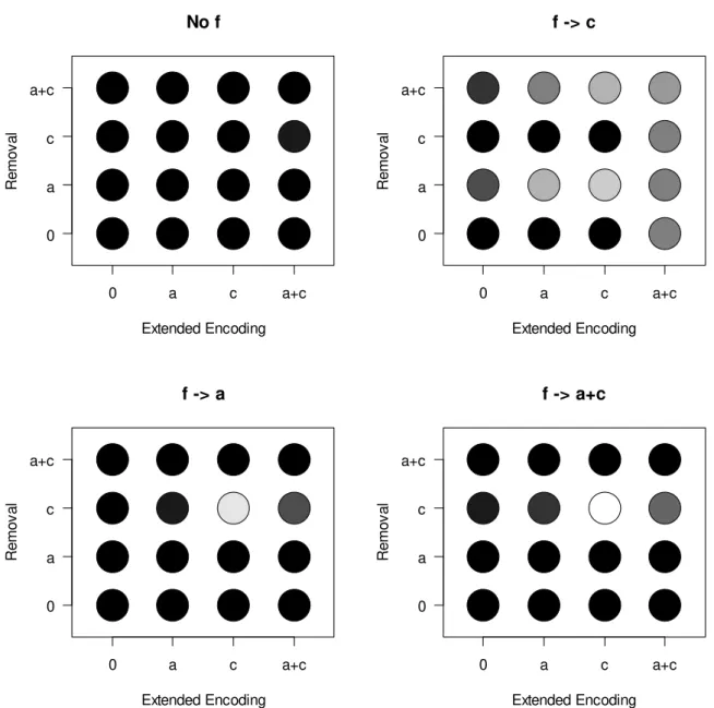
We applied the 64 model versions to the data from each experiment using JAGS 4.2 (Plummer, 2016) for running the MCMC samples, together with the R2jags package (Su, 2015) in R (R_Core_Team, 2017). Model comparison was based on the WAIC information criterion (Watanabe, 2010), which is suited for hierarchical models and has better statistical properties than the more often used DIC (Gelman, Hwang, & Vehtari, 2014). Smaller WAIC values reflect better model fit. Figure 2 illustrates the distribution of the WAIC values over models.

4 _{Sampling of negative values from the Normals could be avoided by truncating them at zero, but in practice we}

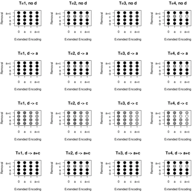
Figure 2: Goodness of fit of the 64 model versions applied to Experiment 1. Gray scale represents difference of each models' WAIC from the smallest (best) WAIC. Darker shading means larger WAIC values, in 10 steps of 10 WAIC points each, so that all WAIC differences > 100 are depicted in black.

Results

Experiment 1. The bar graphs in Figure 3 reflect the behaviorally observed probabilities of choosing a response in each of the five response categories. The empirical probabilities are calculated as the number of responses in each category divided by the number of response candidates in each category. For instance, although the absolute number of distractor in position responses was smaller than the number of other distractor responses, the probability of choosing each individual other distractor was smaller than the probability of choosing each distractor in position, because there were more other distractors in the test array than there were distractors in position.

No f Extended Encoding Re m o v a l 0 a c a+c 0 a c a+c f -> a Extended Encoding Re m o v a l 0 a c a+c 0 a c a+c f -> c Extended Encoding Re m o v a l 0 a c a+c 0 a c a+c f -> a+c Extended Encoding Re m o v a l 0 a c a+c 0 a c a+c

Figure 3: Mean probability of choosing a word from each of the five response categories (bars), with predictions from the best-fitting M3 _{model (red dots) for Experiment 1. P(choice)}

is the probability of choosing each individual word in a given category, so for response categories with more than one word, the proportion of responses in that category was divided by the number of words in the candidate set belonging to that category. Error bars are 95% confidence intervals for within-subjects comparisons (Bakeman & McArthur, 1996). Model predictions are derived from the means of the posterior predictives for each participant and category.

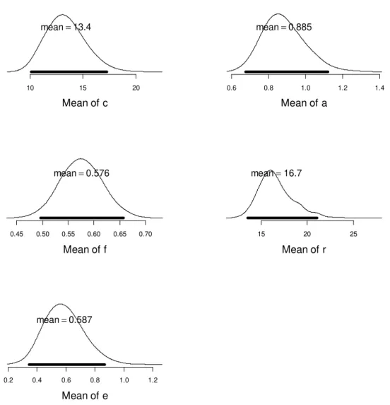
The model with the best fit had an extended-encoding parameter affecting only the binding strength c, a removal rate parameter also affecting only c, and a filter parameter affecting both a and c. The red dots in Figure 3 represent the means of the posterior predictives of the model. The posterior predictives are samples of predicted data obtained with parameter values sampled from their posteriors. Figure 4 shows the posteriors of the parameter means across participants. These distributions are obtained by averaging the posterior parameter values of all individuals at each MCMC sample, thereby generating a sample of their posterior mean.

Several conclusions can be drawn from these results. First, longer free time after distractors increased the number of correct responses at the expense of all error categories (perhaps with the exception of NPLs). The model attributes this effect to extended encoding of item-context bindings, and to removal of distractor activation. The effect of extended

Short Time Long Time

P(Choice) 0.0 0 .2 0.4 0 .6 0.8 1 .0 Correct

Short Time Long Time

P(Choice) 0.00 0.02 0.04 0.06 Other Item

Short Time Long Time

P(Choice) 0.00 0.02 0.04 0.06 Distractor in Position

Short Time Long Time

P(Choice) 0.00 0.02 0.04 0.06 Other Distractor

Short Time Long Time

P(Choice) 0.00 0.02 0.04 0.06 NPL

encoding on c is substantial: We can calculate the increase in binding strength c through extended encoding for each free-time condition C as Δc=c⋅e⋅t_c. Using the means of the posteriors for each parameter, we obtain Δc = 13.4 x 0.59 x [0.2, 1.5] = [1.6, 11.9]. In other words, the long free time of 1.5 s nearly doubled the estimated strength of item-context bindings.

Figure 4: Posterior probability densities of the means of parameter estimates across

participants for the best-fitting M3 _{model of Experiment 1. The distributions were constructed}

by taking the average of all participants' parameter values at each MCMC sampling step, then plotting a smoothed histogram of these averages across all MCMC steps. Thick horizontal bars represent the 95% highest-density interval (HDI) (Kruschke, 2011).

Second, distractors are encoded into working memory, but with only about half the strength compared to memory items, as reflected in the filtering parameter. In addition, distractor-context bindings – but not distractor activation – are removed after encoding. The high removal rate implies that removal of bindings proceeds very rapidly: With r = 16.7, the strength of distractor-context bindings is reduced by 96% after 0.2 s of free time, and virtually eliminated after 1.5 s. The rapid removal rate implies only a negligible difference in

10 15 20 Mean of c mean=13.4 0.6 0.8 1.0 1.2 1.4 Mean of a mean=0.885 0.45 0.50 0.55 0.60 0.65 0.70 Mean of f mean=0.576 15 20 25 Mean of r mean=16.7 0.2 0.4 0.6 0.8 1.0 1.2 Mean of e mean=0.587

distractor-context bindings between the short and the long free-time conditions of this experiment. Therefore, rapid removal is difficult to distinguish from particularly strong filtering of distractor-context bindings at encoding. A further model version, in which

separate filtering parameters fa and fc were applied to a and c, respectively, provided a slightly

better fit to the data of Experiment 1, with an estimate of mean fc = 0.03. To resolve this

ambiguity, in Experiments 2 and 3 we included a condition in which distractors were

identified as such only after they have been encoded into working memory. In this post-cued condition any reduced strength of distractors relative to memory items must be attributed to removal after initial encoding. To foreshadow, Experiments 2 and 3 will confirm that distractor-context bindings are rapidly removed after encoding.

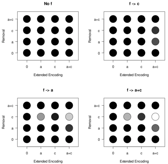
Figure 5: Goodness of fit of the 64 model versions applied to Experiment 2. Gray scale represents difference of each models' WAIC from the smallest (best) WAIC. Darker shading means larger WAIC values, in 10 steps of 10 WAIC points each, so that all WAIC differences > 100 are depicted in black.

Experiments 2 and 3. For both experiments, the model with a filtering parameter applied to both a and c, extended encoding applied to a and c, and removal applied to c only fit the data best. Figure 5 shows the WAIC differences for the models applied to Experiment 2; the equivalent plot for Experiment 3 looks very similar and is not shown to avoid

No f Extended Encoding Re m o v a l 0 a c a+c 0 a c a+c f -> a Extended Encoding Re mo v a l 0 a c a+c 0 a c a+c f -> c Extended Encoding Re m o v a l 0 a c a+c 0 a c a+c f -> a+c Extended Encoding Re mo v a l 0 a c a+c 0 a c a+c

redundancy. The proportions of responses together with the model predictions are presented in Figures 6 and 8, for Experiments 2 and 3, respectively. The posteriors of parameter means are plotted in Figures 7 and 9. The results of both experiments are remarkably consistent with each other. The parameter estimates for c and a roughly match those for Experiment 1; the effect of extended encoding was estimated to be even stronger than in Experiment 1, and affected not only item-context bindings but also item activation. The filtering parameter estimates approximately match the f parameter of Experiment 1.

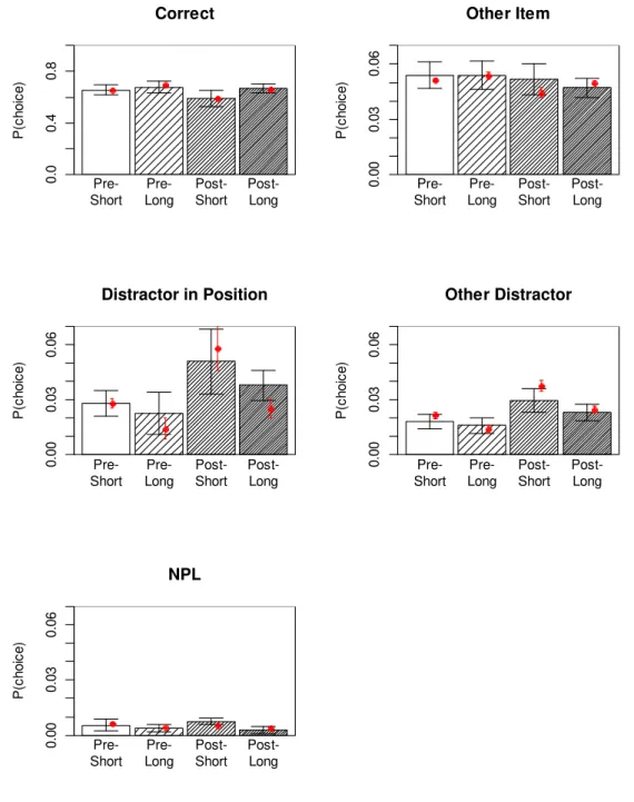
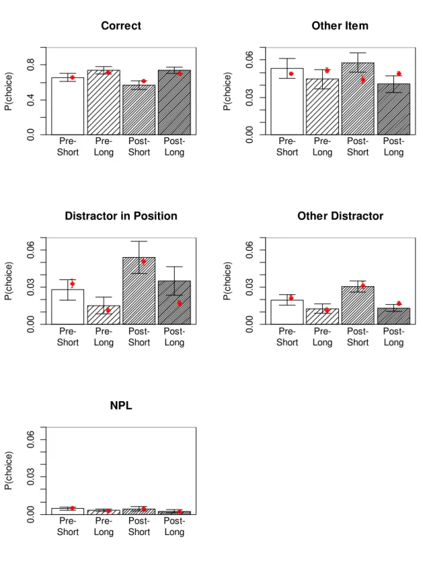
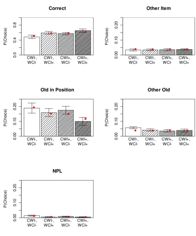
Figure 6: Mean probability of choosing a word from each of the five response categories (bars), with predictions from the best-fitting M3 _{model (red dots) for Experiment 2. See legend}

of Figure 2 for details. Pre = pre-cued condition, Post = post-cued condition, Short = short free time, Long = long free time.

Pre-Short Pre-Long Post-Short Post-Long P (c hoi c e) 0.0 0 .4 0.8 Correct Pre-Short Pre-Long Post-Short Post-Long P (c hoi c e) 0. 00 0. 03 0. 06 Other Item Pre-Short Pre-Long Post-Short Post-Long P (c hoi c e) 0. 00 0. 03 0. 06 Distractor in Position Pre-Short Pre-Long Post-Short Post-Long P (c hoi c e) 0. 00 0. 03 0. 06 Other Distractor Pre-Short Pre-Long Post-Short Post-Long P (ch o ice ) 0. 00 0 .03 0 .06 NPL

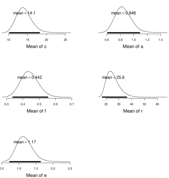
Figure 7. Posterior probability densities of the means of parameter estimates across

participants for the best-fitting M3 _{model of Experiment 2. See legend of Figure 3 for details.}

The removal parameter again implies a very rapid removal process operating only on c. Strong and rapid removal is necessary for the model to explain the relative proportions of selections of memory items and of distractors in the post-cued condition, in which the strength of distractors could only be reduced by removal. Although post-cued distractors intruded into recall more often than pre-cued distractors, the difference was modest, and post-cued

distractors were still chosen much less frequently than memory items, implying that their strength must have been reduced substantially in response to the cue. Because the post-cues were presented only after the distractors have been presented and processed (i.e., after participants made their size judgment on them), this reduction in strength can only be attributed to removal. The large estimates of the removal rate r imply that the removal of distractor-context bindings is nearly complete even after a short free-time interval: The proportional reduction of c through removal, estimated from the means of the parameter posteriors, was about 98% for short, and essentially 100% for long free time.

10 15 20 25 Mean of c mean=14.1 0.6 0.8 1.0 1.2 1.4 Mean of a mean=0.848 0.3 0.4 0.5 0.6 0.7 Mean of f mean=0.442 20 30 40 50 60 Mean of r mean=25.6 0.5 1.0 1.5 2.0 2.5 Mean of e mean=1.17

Figure 8: Mean probability of choosing a word from each of the five response categories (bars), with predictions from the best-fitting M3 _{model (red dots) for Experiment 3. See legend}

of Figure 2 for details. Pre = pre-cued condition, Post = post-cued condition, Short = short free time, Long = long free time.

Pre-Short Pre-Long Post-Short Post-Long P (c hoic e ) 0. 0 0. 4 0. 8 Correct Pre-Short Pre-Long Post-Short Post-Long P (c hoic e ) 0. 00 0. 03 0. 06 Other Item Pre-Short Pre-Long Post-Short Post-Long P (c hoic e ) 0. 00 0. 03 0. 06 Distractor in Position Pre-Short Pre-Long Post-Short Post-Long P (c hoic e ) 0. 00 0. 03 0. 06 Other Distractor Pre-Short Pre-Long Post-Short Post-Long P (c hoic e ) 0. 00 0. 03 0. 06 NPL

Figure 9. Posterior probability densities of the means of parameter estimates across

participants for the best-fitting M3 _{model of Experiment 3. See legend of Figure 3 for details.}

Discussion

Besides demonstrating the usefulness of the M3 _{framework, several substantive}

conclusions can be drawn from Experiments 1 to 3. First, replicating previous experiments (Oberauer, Farrell, et al., 2012), distractors were recalled more often than NPLs. This

demonstrates that distractors are encoded into working memory to some extent, confirming an assumption in the SOB-CS model (Oberauer, Lewandowsky, et al., 2012). The measurement models provide a more detailed picture of this process. Estimates of the filtering parameter show that words known to be distractors during encoding are encoded with reduced strength compared to memory items. This filtering applies equally to activation and binding.

After encoding, distractors are to some extent removed from working memory. Whereas the existence of such a removal process is predicted by the SOB-CS model, the details that emerge from the present experiments do not agree well with that model. In SOB-CS, removal consists of the gradual untying of distractor-context bindings. The measurement

10 15 20 25 Mean of c mean=15 0.4 0.6 0.8 1.0 1.2 1.4 1.6 Mean of a mean=0.815 0.4 0.5 0.6 0.7 0.8 Mean of f mean=0.605 15 20 25 30 Mean of r mean=16.3 2 3 4 5 Mean of e mean=2.6

models instead reveal a very rapid removal of distractor-context bindings. The M3 predicts this removal to be virtually complete after 1.5 s of free time. This might not be entirely accurate: In all three experiments, there was still a somewhat higher probability of recalling a distractor close to the current list position than another distractor even in the long free-time condition; a tendency that the model predictions miss. We explored whether the model prediction could be improved in this regard if removal of distractor-context bindings were modelled as a rapid exponential decline to an above-zero asymptote. We extended the best-fitting model version for Experiments 2 and 3, respectively, by adding the lower asymptote of removal as a further free parameter. This extension improved the model fit slightly for

Experiment 3 (ΔWAIC = 15), but not for Experiment 2 (ΔWAIC < 1).

The measurement models also afford separating the effects of extended item encoding and of distractor removal during free-time intervals. Across all three experiments, memory items gained substantial strength during longer free-time intervals. This was true for free time immediately following each item (Experiment 3), but also for free time following distractors (Experiments 1 and 2), implying that free time can be used to boost memory strength of previously encoded items also after a disruption by an intervening distractor. Extended encoding of memory items contributed much more to the beneficial effect of free time than removal of distractors. This finding demands a revision of the SOB-CS model, in which distractor removal alone accounts for the free-time benefit. At least for words as memoranda, memory strength does not does not remain constant after their initial presentation (1.7 s in the present experiments) but continues to grow during subsequent free-time periods, when the word was no longer visible. Across the three experiments the best-fitting models assumed extended encoding to strengthen either item-context bindings alone (Experiment 1) or both bindings and item activation (Experiments 2 and 3).

Several processes have been proposed in the memory literature that could be responsible for the extended encoding benefit. First, we could assume that articulatory rehearsal boosts memory strength for rehearsed items. Tan and Ward (2008) found that serial recall of words – uninterrupted by distractors – is better when words are presented at a slower rate (5 s vs. 1 s per word). Through an overt-rehearsal procedure Tan and Ward monitored participants' articulatory rehearsal, and found that they engaged in more cumulative rehearsal at the slower presentation rates. Moreover, the extent of cumulative rehearsal correlated positively with serial recall performance. These findings are compatible with the assumption that articulatory rehearsal does not (or not only) protect memory representations from decay, but rather strengthens them beyond their state after presentation (see also Nishiyama & Ukita, 2013). Against this possibility, a series of experiments from the first author's lab found that when cumulative rehearsal was experimentally increased through instruction, it had no beneficial effect on memory (Souza & Oberauer, 2017). Another possible process that could boost memory strength is refreshing, defined as attending to a representation in working memory after its presentation (Johnson, 1992; Raye, Johnson, Mitchell, Greene, & Johnson, 2007). Like rehearsal, refreshing has been invoked as a mechanism for maintaining memory strength in decay theories (Barrouillet et al., 2004), but it could also be conceptualized as a process that increases memory strength above the level reached after initial encoding.

Evidence for that possibility comes from the a study of visual working memory (Souza, Rerko, & Oberauer, 2015): Asking participants to attend to a subset of items in a memory array improved memory for those items. At present it is unclear, however, whether this effect of refreshing is also found for verbal materials, and whether people spontaneously refresh memory representations during free time.

A third possible interpretation of the extended encoding process is as consolidation. Consolidation can be distinguished from initial encoding in that consolidation continues to operate after a mask has erased sensory information from the stimulus (Niewenstein & Wyble, 2014; Ricker & Cowan, 2014). Whereas earlier investigations of "short-term

consolidation" of information in working memory estimated it to be complete after less than a second (Jolicoeur & Dell'Acqua, 1998), subsequent research suggests that consolidation can continue for a longer time (Bayliss et al., 2015; Niewenstein & Wyble, 2014). However, consolidation is assumed to be interrupted by a processing demand that requires central attention, or by encoding of another item (Ricker & Cowan, 2014), and it is not clear whether consolidation can resume after such an interruption. A fourth interpretation of extended encoding is as elaborative rehearsal (Craik & Watkins, 1973), defined as creating a richer semantic representation of the memory material by relating items to each other or to knowledge in long-term memory. Elaboration is known to improve episodic long-term memory (Craik & Tulving, 1975), but so far there is no evidence that it also improves recall from working memory. To conclude, the present experiments provide compelling evidence that some process continues to strengthen item-context bindings, and perhaps also item activation, during free time long after their initial encoding. The nature of this process is not clear, and certainly deserves further investigation.

Experiment 4: Working Memory Updating

In the memory-updating paradigm, an initial set of memory items is updated by replacing individual items with new items. The paradigm can be traced back to the early days of experimental cognitive psychology (Yntema & Mueser, 1962). In individual-differences studies, updating tasks are among the best measures of working-memory capacity (Oberauer, Süß, Schulze, Wilhelm, & Wittmann, 2000; Wilhelm, Hildebrandt, & Oberauer, 2013). Here we used a version closely modeled after Kessler and Meiran (2006). Participants encoded an initial set of four words displayed across a row of four frames, and subsequently replace them with new words that are displayed one by one in individual frames in a random sequence. At the end participants try to recall the last word in each frame.

In a previous series of experiments using this task in a self-paced mode, Ecker and colleagues were able to separate two processes involved in working-memory updating: Removal of the old representation and encoding of the new one (Ecker, Lewandowsky, & Oberauer, 2014; Ecker, Oberauer, & Lewandowsky, 2014). In these experiments, each new stimulus was preceded by a cue indicating the frame in which the stimulus will appear. This cue informed participants about which old item in the current memory set will be replaced next, but did not yet reveal the new item. Participants appear to use the time between the cue and the new memory item to remove the old item. This is shown by two findings: First, after a

longer cue-stimulus-interval participants took much less time to update memory once the new stimulus was given. Second, if the new stimulus was similar – or even identical – to the old stimulus it replaced, updating times were faster, but this similarity advantage was eliminated by a long cue-stimulus interval (Ecker, Lewandowsky, et al., 2014; Ecker, Oberauer, et al., 2014). Our aim for Experiment 4 was to apply the M3 _{framework to the updating paradigm}

and to extend it by parameters measuring the removal of old items and the encoding of new items.

Design

The M3 _{framework is so far applicable only to response choice data, not to response}

times. Therefore, we did not use the self-paced updating task of Ecker and colleagues, but a computer-paced version of the same task. After presentation of the initial four memory words – displayed from left to right across a row of four frames – participants saw a series of further words displayed one by one in randomly selected frames. Each new word was presented for 0.5 s. For each new word participants had to replace the word they remembered for that frame by the new word. Each new word was preceded by a cue indicating in which frame it would appear (a fixation cross in the center of the frame, displayed for 0.2 s). The length of the series of new words was unpredictable so that participants had to expect to be tested at any moment – this served to discourage them from not attending to the earlier words in the series. The design crossed a variation of the cue-word interval (0.1 vs. 1.1 s after the offset of the cue) with a variation of the interval between presentation of a new word and the onset of the next cue in another frame (word-cue interval, 0.1 vs. 1.1 s after offset of the word). The purpose of these manipulations was to vary the time for removal of the old item (cue-new word interval) and the time for encoding the new item (new word-next cue interval).

At the end of a series of updating steps, memory was tested by presenting participants with an array of 12 words – the four last words in each frame, the four next-to-last words (which we will refer to as "old words"), and four NPLs. The four frames were probed in a random order, and participants were asked to select the last word for the probed frame from the 12 candidates. We sorted their responses into five categories: Correct words, other words from the set of last words, old words in the probed frame, other old words, and NPLs.

Procedural details of the experiment are provided in the Appendix. Measurement Models for Memory Updating

We extended the basic model by three processes. First, as for the complex-span

models, we included an extended-updating process to capture the increase of memory strength for both activation and item-context bindings during free time te following presentation of a

new word. Second, we included a process of removing the old item after it has been

identified by the cue. Removal was modelled as an exponential reduction of memory strength during the removal interval tr. Third, we include a parameter d that reflects the proportional

weakening of the old item through encoding of the new item. This latter process differs from removal in that it is not time dependent: The same proportional reduction of c and a of old items is assumed for all experimental conditions. One motivation for introducing this