803
Journal homepage: http://www.journalijar.com INTERNATIONAL JOURNAL OF ADVANCED RESEARCHRESEARCH ARTICLE
Spatio-Temporal Change Detection Analysis of Land-use and Land cover: A study of
Mysore-Mandya corridor region
Ali Boloor1 and Asima Nusrath2
1.Ph.D. Research Scholar, Department of Studies in Geography, University of Mysore, Manasagangotri, Mysore - 570006, Karnataka, India
2.Professor in Department of Studies in Geography, University of Mysore, Manasagangotri, Mysore – 570006, Karnataka, India
Manuscript Info
Abstract
Manuscript History:
Received: 25 September 2015 Final Accepted: 22 October 2015
Published Online: November 2015
Key words:
Land use/Land cover, corridor region, accuracy assessment, land transits, change detection
*Corresponding Author
Ali Boloor
The present study has been conducted to analysis the land use and land cover of Mysore-Mandya corridor region between the years 1991 and 2014. The study has been done using remote sensing data and GIS techniques. The necessary satellite images (1991, 2001 and 2014) have been obtained from the United States of Geological Survey website and the GIS analysis has been done in ERDAS. The downloaded satellite has been corrected atmospherically and radio-metrically using ATCOR module in ERDAS. After preparing the corrected base imagery, supervised image classification has been carried out using maximum livelihood algorithm. To prove the accuracy of the classification result, the error matrix and Kappa index have been applied from which the classification accuracy was 95.91 per cent. The spatial extension LULC analysis showed that, the built-up land use has been increasing continuously while other land uses have been decreasing. The land transit analysis depicts the high conversion of vegetation and waste land into built-up during the study period. Finally, decadal wise comparison shows that, during the second period of study (2001 – 2014) the intensity of conversion is higher than the first period (1991 – 2001) for the land use categories.
Copy Right, IJAR, 2015,. All rights reserved
INTRODUCTION
The land covers on the earth surface have been altering from the origin of the planet while land use has been changing ever since human started to live on a particular place. The study of land use and cover can help to manage the present as well as to take necessary actions for the future. (Zhou, Wu, & Peng, 2012). The expansion of population and their needs are altering the limited land and soil resources for agriculture, urban and industrial uses. Thus, the information regarding the rate and kind of shifting land resources is mandatory for proper management, planning and regularization of the use of such resources (Gautam & Narayanan, 1983; Gong et al., 2013).
The studies of land use and land cover using satellite imagery is very popular among the scientific communities as it is cost effective and technologically sound (de Sherbinin et al., 2002; L. Yang, Xian, Klaver, & Deal, 2003; Xiaojun Yang & Liu, 2005). Extensive research have been directed towards urban change detection by employing the remotely sensed imagery (for example; (Gomarasca, Brivio, Pagnoni, & Galli, 1993; Green, Kempka, & Lackey, 1994; Lo & Shipman, 1990; Royer, Charbonneau, & Bonn, 1988; Todd, 1977; Toll, 1985; Toll, Royal, & Davis, 1981; Xlaojun Yang, 2002; Xiaojun Yang & Liu, 2005; Yeh & Li, 1997). Remotely sensed data have been used to characterize patterns of land cover changes at scales from sporadic meters to few degrees in latitude by
804
longitude depending on the sensors (Council, 2008). Satellite imagery offers a historical and recent perspective on landscape dynamics (Peterson, Egbert, Price, & Martinko, 2004).LAND USE LAND COVER CHANGE DETECTION
The process of change detection identifies the modifications in the two sets of images taken from different time period. The process considers several factors namely the nature of the problem comprised in change detection, image processing method, selection of suitable variables and algorithms (Lu, Li, & Moran, 2014).
Several change detection techniques are developed and used by researchers. Notably the post-classification image comparison (Fichera, Modica, & Pollino, 2012; Rawat & Kumar, 2015; Tian et al., 2005), object based change detection (Blaschke, 2005), cross-correlation (Wang, Chen, Gong, Shimazaki, & Tamura, 2009; Z. Yang & Mueller, 2007), improved change-vector analysis (Chen, Gong, He, Pu, & Shi, 2003), texture analysis (Erener & Düzgün, 2009), multivariate alteration detection (Nori, Elsidding, & Niemeyer, 2008) and change-vector analysis (Setiawan & Yoshino, 2012) are some of the change detection approaches.
The post classification comparison technique is the most logical method for change detection, which involves the cataloguing of each selected images independently followed by comparison of corresponding pixel value to identify areas where change has occurred (Roostaei & Kamran, 2012; Weismiller, Kristof, Scholz, Anuta, & Momin, 1977). The accuracy assessment of the classification to the real world can be analyzed using the error matrix system, through which the percentage of the categorization precision can be obtained.
Therefore, the present study has been conducted to analysis the land use and land cover changes along the Mysore-Mandya corridor region, where rapid changes have been taken recently by the construction of Bangalore– Mysore Industrial Corridor (Goldman, 2011).
METHODOLOGY
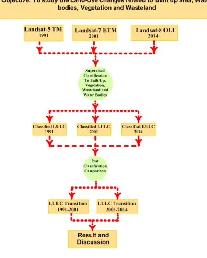
The selected change detection method for the present study employs the independent thematic classification images taken at two different time spans, which can generate the results with ‘from-to’ change information that is easy to interpret. The correction of the atmosphere and sensor errors in the diverse satellite imageries would improve the accuracy of results. The methodology flowchart is displayed in figure 1.
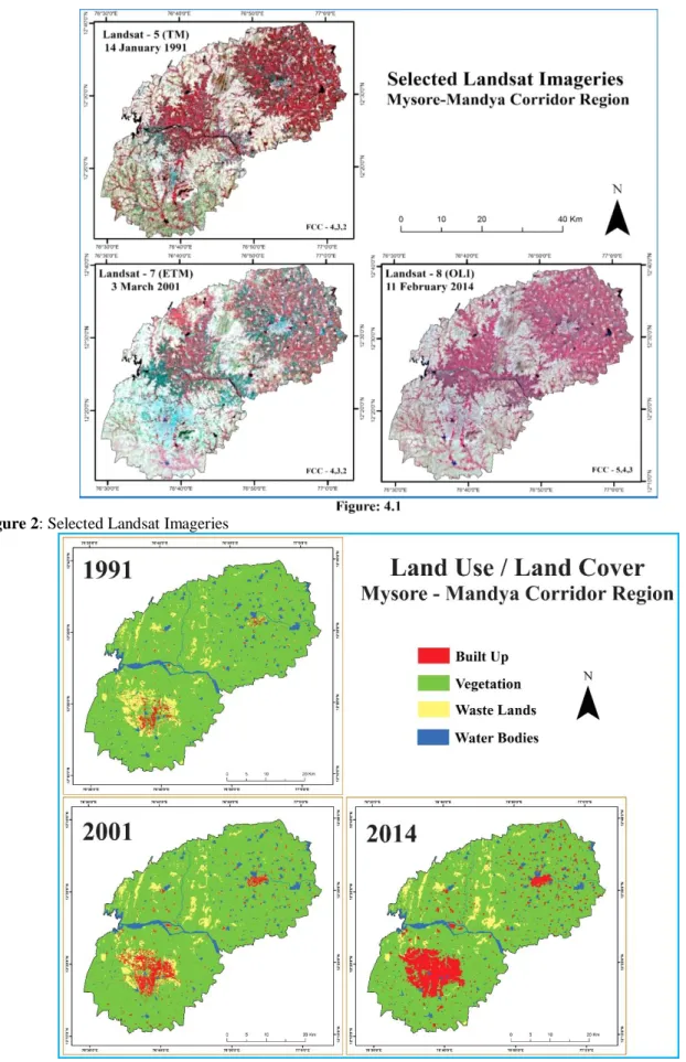
To unearth the existing LULC in the study area, the satellite images of 1991, 2001 and 2014 have been corrected atmospherically, radio-metrically and geometrically. The atmospheric and radiometric corrections have been done employing the ATCOR module in ERDAS and geometric correction has been done through the ERDAS itself. The Figure 2 shows the details of the Landsat based map used in the present study which are downloaded from the USGS and they are likely to be as follows:
For the first time period, 14th January 1991 Landsat-5 satellite data has been used. For the second time period, 3rd March 2001 Landsat-7 satellite data has been utilized. For the final time period, 11th February 2014 data Landsat-8 satellite has been employed.
To obtain higher accuracy of LULC, the base data should be on the similar scale or same spatial resolution which is of 30 meters for the present study. After the preparation of the base data, the supervised classification using Maximum Likelihood classification is implemented to classify the imageries. The supervised classification is a popular approach which is highly handled in India as well as in other countries (Maktav & Erbek, 2005), for Istanbul, Turkey; (Nori et al., 2008) for El Rawashda forest, Sudan; (Uma & Mahalingam, 2011) for Kanchipuram District, Coastal Stretch, Tamil Nadu, India). The training sample locations were identified for the year 2014 as 120 sample sites (Area of Interest) for Built-Up, 132 for Vegetation, 102 for Waste land and 57 for Water bodies have been collected and from this signature, a file has been created in ERDAS for the purpose of further analysis.
ACCURACY ASSESSMENT
The result of classification cannot be accepted without proving the accuracy of the classification, therefore the present study has used the Confusion Matrix and Cohen’s Kappa, which is highly accepted and followed by several researchers for the accuracy assessment of LULC studies (Hollister, Gonzalez, Paul, August, & Copeland, 2004; Kaul & Sopan, 2012).
The Cohen’s Kappa is used to calculate the agreement between the two individual variables that measures the same land-use. The result of Kappa is less than or equal to 1 with the values near to 1 represents the perfect agreement while those near to 0 represents the worst agreement. The Table 1 accentuates on the error matrix table that is prepared to measure the accuracy of the classification.
805
Before selecting the samples, it is necessary to decide upon the number of samples for each class. Therefore, the study has followed rule of the thumb method to assign the number of samples. The total number of samples for each class has been determined based on the area covered, that is, for larger areas, a higher number of samples and lesser for small areas (for example: samples for vegetation are 158 with an area of 1543.81 km2 and 31 samples for water bodies with an area of 72.53 km2).As stated in the Table 1, an overall 269 points have been taken from the classified images randomly, from which, 32 samples belong to the waste land, 48 belong to the built-up section, 31 are attributed to the water bodies and 158 are related to the vegetation. For these selected samples, points of latitude and longitude have been identified and transferred to hand-held GPS for field verification. For ground verification and reference recording, the researcher has visited all the chosen sample areas. Finally, classified image results and the ground verification information have been used to prepare the error matrix and Kappa statistics (Figure 3).
The overall accuracy has been analyzed after the class wise accuracy assessment; the result represents 95.91 per cent of the overall accuracy, which is more than the minimum numeral of interpretation accuracy of 85 per cent (ANDERSON, HARDY, ROACH, & WITMER, 1976; Rao, GAUTAM, R.L.Karale, & Sahai, 1991). The ‘kappa’ calculation marks the value of 0.932 which is equal to 93 per cent.
806
Figure 2: Selected Landsat Imageries807
Table 1: Accuracy Assessment of LULCS. No Classified LULC Wasteland Built
Up
Water
Bodies Vegetation Total User Accuracy
1 Wasteland 29 2 0 1 32 90.63 2 Built Up 2 45 0 1 48 93.75 3 Water Bodies 1 0 30 0 31 96.77 4 Vegetation 3 0 1 154 158 97.47 Total 35 47 31 156 269 Producer Accuracy 82.86 95.74 96.77 98.72 Overall Accuracy = 95.91 Kappa Result = 0.932
DISCUSSION OF LULC RESULTS
After the confirmation of LULC classification result, the area covered by each class in the selected years has been scrutinized using ArcGIS and presented in Table 2 and Figure 4. The year wise classified result shows that during 1991, 2001 and 2014 the built up area has been increasing as 34.01 km2, 83.26 km2 and 180.25 km2 respectively, while other land use classes’ vegetation, wasteland and water bodies have shown decrease for the respective three decades.
Table 2: Temporal Land use and Land Cover – Mysore-Mandya Corridor Region
S.No Classes Area (km
2 ) Changes (km2) 1991 2001 2014 1991 - 2001 2001-2014 1991-2014 1 Built Up 34.01 83.26 180.25 49.25 96.99 146.24 2 Vegetation 1634.35 1597.54 1543.8 -36.81 -53.74 -90.55 3 Waste Land 127.03 121.23 83.47 -5.80 -37.76 -43.56 4 Water Bodies 84.68 78.04 72.55 -6.64 -5.49 -12.13
Figure 4: Land Use Land Cover (1991-2014)
Moreover, post classification comparison method has been used to calculate the LULC changes between the selected years and the change values are given in Table 2. The temporal changes of the classified LULC results prove that except built up areas all others having negative change. The increase in built up is systematically compensated by the decrease in the area of vegetation, waste land and water bodies. This indicates the positive growth in built up land use and decreasing rate of vegetation is compensated by the escalating trend in the built up area. Similarly, wasteland and water bodies shows decreasing trend following that of vegetation.
SPATIAL EXTENSION: Table 3, depicts the results of the spatial extension of each classified class in the study area. It is clear that even though vegetation has covered more than 80 per cent of the corridor region in all the three observed periods, its area has incessantly shrunk (Figure 5) followed by the waste land and water bodies. The built up has shown a positive augmentation in its area which was 1.81 per cent in 1991 and has gone up to 4.43 per cent to 9.59 per cent for the year 2001 and 2014.
808
Table 3: Temporal Land use and Land Cover – Area and Rate of Change in PercentageS.No Classes Area (%) Changes (%)
1991 2001 2014 1991 - 2001 2001-2014 1991-2014
1 Built Up 1.81 4.43 9.59 59.15 53.80 81.13
2 Vegetation 86.93 84.97 82.11 -2.30 -3.48 -5.86
3 Waste Land 6.76 6.45 4.44 -4.78 -45.23 -52.18
4 Water Bodies 4.50 4.15 3.86 -8.50 -7.56 -16.71
Source: Result of LULC Analysis
Figure 5: Land use land cover change CHANGE IN PERCENTAGE OF LULC
The variation in the percentage of land use and land cover (Table 3) has been calculated to identify the changes that have been taken place in the study area for the period of 1991-2001, 2001-2014 and for 1991-2014. The built up has shown a positive change which was 59.15 per cent in 1991-2001 and 53.80 per cent for 2001-2014, followed by an overall rate of 1991-2014 where the growth recorded reached up to 81.13 per cent, whereas a marginal negative change is noticed in vegetation that is -2.3 per cent for the period of 1991-2001 noted a further decrease of -3.48 per cent in its area in 2001-2014. Ultimately, for the general period, the figure has reduced to -5.86 per cent.
LULC TRANSITION FROM 1991 TO 2001
The analysis of LULC transition helps to find out how the transformation of a particular land use or land cover has been shifted in to another category over the period of time. The table 4 shows the LULC transition that has taken place between the classified classes for the selected years (Figure 6) of the corridor region. The analysis result for the year 1991 to 2001 represents that totally 55.62 km2 of vegetation area has been converted into other categories from which 25.87 km2 turned into built-ups, highest area of 29.17 km2 into waste land and the least of 0.58 km2 into water bodies. The conversion of the area of the waste land shows that 40.84 km2 areas have been transfigured into other categories, as highest area of 29.36 km2 into built-up, 11.46 km2 into vegetation and 0.02 km2 into water bodies. Further the transition trend in the water bodies reveals that 7.01 km2 of areawere converted for other uses, as 0.56 km2 into built-up, 5.25 km2 into vegetation and 1.20 km2 into waste land.
The general assessment of the LULC transition for 1991 to 2001 clearly states that larger quantity of vegetation and waste land have been converted into built-up lands, a hefty amount of vegetation land has been converted into waste land and notable amount of waste land has been converted into vegetation. After the analysis of each class areal transition to another class, the percentage of change occurred from the total area has been calculated and analyzed is as follows.
Table 4 indicates the transition between the vegetation and built-up areas. The tabled data highlights that 25.87 km2 of the vegetation land in 1991 has been systematically converted into built-up within 2001. During the year 1991, the total area of vegetation was 1634.35 km2, that is, (25.87/1634.35)*100, which derives the answer of 1.58. This figure means that 1.58 per cent of the vegetation territory from the total area has been transformed to built -up from 1991 to 2001. Highest change of 1.78% of vegetative area has been transferred into waste land. The percentage wise calculation of each class transition clearly explains that 23.12 per cent of the waste land has been rehabilitated into built up. Following the trends, water bodies have been converted to a highest rate of 6.20 per cent
809
into vegetation. The overall assessment of the percentage of the recurring transition describes that waste land were highly converted trailed by water bodies and vegetation.Table 4: LULC Transition - Mysore-Mandya Corridor Region
S. No. Transition 1991-2001 (km2) 2001-2014 (Km2) 1991-2001 (%) 2001-2014 (%)
1 Built Up to Built-Up 34.01 83.26 Nil Nil
2 Vegetation to Built-Up 25.87 42.90 1.58 2.69
3 Vegetation to Vegetation 1578.56 1533.32 96.59 95.98
4 Vegetation to Waste Lands 29.17 15.52 1.78 0.97
5 Vegetation to Water Bodies 0.58 3.34 0.04 0.21
6 Waste Lands to Built-Up 29.36 55.78 23.12 46.01
7 Waste Lands to Vegetation 11.46 0.12 9.02 0.10
8 Waste Lands to Waste Lands 86.17 64.97 67.83 53.59
9 Waste Lands to Water Bodies 0.02 0.21 0.02 0.18
10 Water Bodies to Built-Up 0.56 0.13 0.67 0.17
11 Water Bodies to Vegetation 5.25 8.57 6.20 10.98
12 Water Bodies to Waste Lands 1.20 0.00 1.42 0.00
13 Water Bodies to Water Bodies 77.42 68.97 91.42 88.37
Source: Analytical Result
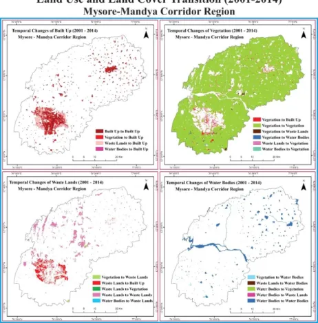
Figure 6: Land Use Land Cover Transition (1991 – 2001) LULC TRANSITION FROM 2001 TO 2014
The transition calculation for the years 2001 to 2014 denotes (Table 4) that totally 61.76 km2 areas of vegetation have been transformed into other (Figure 7) categories, which are higher than the previous decade. 42.90
810
km2 areas have been converted into built-up terrains. The transition in the waste land shows that 55.78 km2 have been converted into built-up. Finally, the transition of water bodies into other classes depicts that 8.57 km2 were converted into vegetation.The overall assessment of transition within 2001 to 2014 depicts that the subsequent conversion of vegetation into built-up, waste lands into built-up and water bodies into vegetation nearly doubled contrasted to the previous decade. From this analysis, it can be concluded that the major reason for the LULC changes in the study area was the undeniable influence of the anthropogenic activities, which were more elevated than that of the previous decade.
The percentage transition of each class illustrates that 2.69 per cent from the total vegetative area has been converted into built up. The transition of waste land displays 46.01 per cent has been changed into built up. Lastly, the transition of water bodies represents that 0.17 per cent has been converted into built up and 10.98 per cent into vegetation. The percentage evaluation of the transition between 2001 and 2014 depicts that the waste land have transited highly into built up, which is almost 50 per cent of its total area and the water bodies into vegetation which consists of 11 per cent.
Figure 7: Land Use Land Cover Transition (2001 - 2014)
CONCLUSION
The study of changes in land use and land cover in Mysore-Mandya corridor depicts that, spatial extension wise the built-up land use has been increasing continuously while other land uses have been decreasing constantly, notably the increasing built-up land use between the years 1991 and 2001 was 49.25 km2; then between the years 2001 and 2014 was 96.99 km2 this states that, the changes had occurred highly in the second period than the first period. The result of land transition represents that, during the period 1991 to 2001 vast area of vegetation and waste land have been converted into built-up, but it is less when compared with the second period between 2001 and 2014 when rapid amount of transition had occurred. This result from the anthropogenic activities of increasing built -up land use on vegetation and water bodies are higher during the second period. Based on the results of present study it can be concluded that, the changes of LULC in the study area is happening like other places, but the conversion of vegetation and waste land into the built-land is high which may cause problem to the environment if the same trend continues. From the study it can be suggested that, there is a need to analyses the existing land conversion policies
811
and rules and implement new necessary policies and rules to control the high rate of conversion of vegetation in built-up land which may protect the future environment.REFERENCE
ANDERSON, J. R., HARDY, E. E., ROACH, J. T., & WITMER, R. E. (1976). A Land Use and Land Cover Classification System for Use with Remote Sensor Data.
Blaschke, T. (2005). Towards a framework for change detection based on image objects. Göttinger Geographische Abhandlungen, 113, 1-9.
Chen, J., Gong, P., He, C., Pu, R., & Shi, P. (2003). Land-use/land-cover change detection using improved change-vector analysis. Photogrammetric Engineering & Remote Sensing, 69(4), 369-379.
Council, N. R. (2008). Earth observations from space: The first 50 years of scientific achievements., from http://www.nap.edu/catalog/11991.html.
de Sherbinin, A., Balk, D., Yager, K., Jaiteh, M., Pozzi, F., Giri, C., & Wannebo, A. (2002). A CIESIN thematic guide to social science applications of remote sensing. Columbia University, New York, NY.
Erener, A., & Düzgün, H. S. (2009). A methodology for land use change detection of high resolution pan images based on texture analysis.
Fichera, C. R., Modica, G., & Pollino, M. (2012). Land Cover classification and change-detection analysis using multi-temporal remote sensed imagery and landscape metrics. European Journal of Remote Sensing, 45(1), 1-18.
Gautam, N. C., & Narayanan, E. R. (Eds.). (1983). Satellite remote sensing techniques for natural resources survey. Allahabad geophysical society,177 - 181.
Goldman, M. (2011). Speculative urbanism and the making of the next world city. International Journal of Urban and Regional Research, 35(3), 555-581.
Gomarasca, M. A., Brivio, P. A., Pagnoni, F., & Galli, A. (1993). One century of land use changes in the metropolitan area of Milan (Italy). International Journal of Remote Sensing, 14(2), 211-223. doi: 10.1080/01431169308904333
Gong, P., Wang, J., Yu, L., Zhao, Y., Zhao, Y., Liang, L., . . . Chen, J. (2013). Finer resolution observation and monitoring of global land cover: first mapping results with Landsat TM and ETM+ data. International Journal of Remote Sensing, 34(7), 2607-2654. doi: 10.1080/01431161.2012.748992
Green, K., Kempka, D., & Lackey, L. (1994). Using remote sensing to detect and monitor land-cover and land-use change. Photogrammetric engineering and remote sensing, 60(3), 331-337.
Hollister, J. W., Gonzalez, M. L., Paul, J. F., August, P. V., & Copeland, J. L. (2004). Assessing the accuracy of National Land Cover Dataset area estimates at multiple spatial extents. Photogrammetric Engineering & Remote Sensing, 70(4), 405-414.
Kaul, H. A., & Sopan, I. (2012). Land Use Land Cover Classification and Change Detection Using High Resolution Temporal Satellite Data. Journal of Environment, 1(04), 146-152.
Lo, C., & Shipman, R. L. (1990). A GIS approach to land-use change dynamics detection. Photogrammetric engineering and remote sensing, 56(11), 1483-1491.
Lu, D., Li, G., & Moran, E. (2014). Current situation and needs of change detection techniques. International Journal of Image and Data Fusion, 5(1), 13-38. doi: 10.1080/19479832.2013.868372
Maktav, D., & Erbek, F. (2005). Analysis of urban growth using multi‐temporal satellite data in Istanbul, Turkey. International Journal of Remote Sensing, 26(4), 797-810.
Nori, W., Elsidding, E., & Niemeyer, I. (2008). Detection of land cover changes using multi-temporal satellite imagery. The International Archives of the Photogrammetry, Remote Sensing and Spatial Information Sciences, 37(B7), 947-952.
Peterson, D. L., Egbert, S. L., Price, K. P., & Martinko, E. A. (2004). Identifying historical and recent land-cover changes in Kansas using post-classification change detection techniques. Transactions of the Kansas Academy of Science, 107(3), 105-118.
Rao, D. P., GAUTAM, N. C., R.L.Karale, & Sahai, B. (1991). IRS-1A Application for land use/land cover mapping in India Current Science, 61(3&4), 153-161.
Rawat, J. S., & Kumar, M. (2015). Monitoring land use/cover change using remote sensing and GIS techniques: A case study of Hawalbagh block, district Almora, Uttarakhand, India. The Egyptian Journal of Remote Sensing and Space Science, 18(1), 77-84. doi: http://dx.doi.org/10.1016/j.ejrs.2015.02.002
Roostaei, S., & Kamran, K. V. (2012). Evaluation of object-oriented and pixel based classification methods for extracting changes in urban area. INTERNATIONAL JOURNAL OF GEOMATICS AND GEOSCIENCES, 2(3), 738-749.
812
Royer, A., Charbonneau, L., & Bonn, F. (1988). Urbanization and Landsat MSS albedo change in theWindsor-Québec corridor since 1972. International Journal of Remote Sensing, 9(3), 555-566. doi: 10.1080/01431168808954875
Setiawan, Y., & Yoshino, K. (2012). Change detection in land-use and land-cover dynamics at a regional scale from MODIS time-series imagery. ISPRS Annals of Photogrammetry, Remote Sensing and Spatial Information Sciences, 1, 243-248.
Tian, G., Liu, J., Xie, Y., Yang, Z., Zhuang, D., & Niu, Z. (2005). Analysis of spatio-temporal dynamic pattern and driving forces of urban land in China in 1990s using TM images and GIS. Cities, 22(6), 400-410. doi: http://dx.doi.org/10.1016/j.cities.2005.05.009
Todd, W. J. (1977). Urban and regional land use change detected by using Landsat data. Journal of Research of the US Geological Survey, 5(5), 529-534.
Toll, D. L. (1985). Landsat-4 Thematic Mapper scene characteristics of a suburban and rural area. Photogrammetric engineering and remote sensing, 51, 1471-1482.
Toll, D. L., Royal, J. A., & Davis, J. B. (1981). Urban area update procedures using Landsat data. Paper presented at the In Proceedings of the Fall Technical Meeting of the American Society of Photogrammetry held in Niagra Falls, Canada. , Falls Church, Virginia: ASP, pp. RS-E1-17.
Uma, J., & Mahalingam, B. (2011). Spatio-Temporal changes of Land use and Land cover analysis using Remote Sensing and GIS: A case study of Kanchipuram District Coastal Stretch - Tamil Nadu. International Journal of Geomatics & Geosciences, 2(1), 188-195.
Wang, L., Chen, J., Gong, P., Shimazaki, H., & Tamura, M. (2009). Land cover change detection with a cross‐correlogram spectral matching algorithm. International Journal of Remote Sensing, 30(12), 3259-3273.
Weismiller, R., Kristof, S., Scholz, D., Anuta, P., & Momin, S. (1977). Change detection in coastal zone environments. Photogrammetric engineering and remote sensing, 43(12).
Yang, L., Xian, G., Klaver, J. M., & Deal, B. (2003). Urban land-cover change detection through sub-pixel imperviousness mapping using remotely sensed data. Photogrammetric Engineering & Remote Sensing, 69(9), 1003-1010.
Yang, X. (2002). Satellite monitoring of urban spatial growth in the Atlanta metropolitan area. Photogrammetric engineering and remote sensing, 68(7), 725-734.
Yang, X., & Liu, Z. (2005). Use of satellite-derived landscape imperviousness index to characterize urban spatial growth. Computers, Environment and Urban Systems, 29(5), 524-540. doi:
http://dx.doi.org/10.1016/j.compenvurbsys.2005.01.005
Yang, Z., & Mueller, R. (2007). SPATIAL-SPECTRAL CROSS-CORRELATION FOR CHANGE DETECTION---A CASE STUDY FOR CITRUS COVERAGE CHANGE DETECTION. Paper presented at the ASPRS 2007 Annual Conference Tampa.
Yeh, A. G. o., & Li, X. (1997). An integrated remote sensing and GIS approach in the monitoring and evaluation of rapid urban growth for sustainable development in the Pearl River Delta, China. International Planning Studies, 2(2), 193-210. doi: 10.1080/13563479708721678
Zhou, T., Wu, J., & Peng, S. (2012). Assessing the effects of landscape pattern on river water quality at multiple scales: A case study of the Dongjiang River watershed, China. Ecological Indicators, 23, 166-175. doi: http://dx.doi.org/10.1016/j.ecolind.2012.03.013