IRISS at
CEPS/INSTEAD
An Integrated Research
Infrastructure in the Socio-Economic
Sciences
BAYESIAN QUANTILE REGRESSION:
AN APPLICATION TO THE WAGE DISTRIBUTION IN
1990s BRITAIN
by
Keming Yu, Philippe Van Kerm and Jin Zhang
IRISS WORKING PAPER SERIES
No. 2004-10
IRISS-C/I
An Integrated Research Infrastructure in the
Socio-Economic Sciences at CEPS/Instead,
Luxembourg
Project supported by the European Commission and the
Ministry of Culture, Higher Education and Research
(Luxembourg)
What is IRISS-C/I?
IRISS-C/I is a visitors’ programme at CEPS/INSTEAD, a policy and research centre based in Luxembourg. Its mission is to organise short visits of researchers willing to undertake empirical research in economics and other social sciences using the archive of micro-data available at the
Centre.
In 1998, CEPS/INSTEAD has been identified by the European Commission as one of the few Large Scale Facilities in the social sciences, and, since then, IRISS-C/I fellowships offer researchers (both junior and senior) the opportunity to spend time carrying out their own research using the local research facilities. The expected duration of visits is in the range of 2 to
12 weeks.
During their stay, visitors are granted access to the CEPS/INSTEAD archive of public-use micro-data (primarily internationally comparable longitudinal surveys on living conditions) and to
extensive data documentation. They are assigned an office (shared or single) and have networked access to a powerful computation server that acts as host for the data archive and supports an array of commercial and open-source statistical software packages. Scientific and
technical assistance is provided by resident staff.
Research areas
Survey and panel data methodology; income and poverty dynamics; gender, ethnic and social inequality; unemployment; segmentation of labour markets; education and training; social protection and redistributive policies; impact of ageing populations; intergenerational relations;
regional development and structural change.
Additional information
IRISS-C/I
B.P. 48 L-4501 Differdange (Luxembourg) Email: [email protected]
Bayesian quantile regression:
An application to the wage distribution in 1990s Britain
Keming Yu∗
University of Plymouth, UK
Philippe Van Kerm
CEPS/INSTEAD, G.-D. Luxembourg
Jin Zhang
University of Manitoba, Canada
Summary. This paper illustrates application of Bayesian inference to quantile
regres-sion. Bayesian inference regards unknown parameters as random variables, and we describe an MCMC algorithm to estimate the posterior densities of quantile regression parameters. Parameter uncertainty is taken into account without relying on asymptotic approximations. Bayesian inference revealed effective in our application to the wage structure among working males in Britain between 1991 and 2001 using data from the British Household Panel Survey. Looking at different points along the conditional wage distribution uncovered important features of wage returns to education, experience and public sector employment that would be concealed by mean regression.
AMS (2000)subject classification. Primary 62J02;secondary 62C10, 62P20, 62P25.
Keywords and phrases. Quantile regression, Bayesian inference, wage distribution, MCMC.
1
Introduction
It is now widely acknowledged that quantile regression can be a very useful item in an econometrician’s toolbox when analysing income and wage distribution issues. These models may reveal evidence otherwise concealed by standard mean regression. Stan-dard regression methods provide a simple and informative way of exploring mean wage returns to important variables such as education, tenure, etc. But the mean return may not be our prime interest, or we may want to supplement information about the mean with information about the whole (conditional) distribution when we have reasons to expect substantial heterogeneity among agents sharing the same observed characteris-tics. For example, one thing is to estimate the mean wage among, say, all “IT industry male workers in the UK in 2000.” But, given that the distribution of wage is typi-cally skewed to the right with few large wages, it is also informative to know the wage level that splits this group of people in two equal-sized groups –the median may be a better description of a ‘typical’ case. Or, if we expect substantial heterogeneity of experiences, we may also be interested in the wage above which are 90 percent of such
∗Address for correspondence: Department of Mathematics and Statistics, University of Plymouth,
workers’ wages –an indication about how low wage may tend to be, or the wage above which are 10 percent of such workers’ wages –an indication about how high wage can be–, etc. This collapses to estimating various quantiles of the wage distribution condi-tionally on being an “IT industry male worker in the UK in 2000.” Quantile regression models have also been advocated on the ground that they are more robust to outliers than mean regression. These methods have been recently used extensively in research on wage distribution with applications, e.g. to the US by Buchinsky (1994), to the UK by Disney and Gosling (1998) or to Portugal by Machado and Mata (2002).
Bayesian inference combined with Markov Chain Monte Carlo algorithms have be-come increasingly popular and Bayesian approaches to quantile regression have been developed by Yu and Moyeed (2001). The two major advantages of Bayesian inference for quantile regression models, as compared to the classical methods, are that (i) it does not rely on approximations to the asymptotic variances of the estimators, and (ii) it provides estimation and forecasts which fully take into account parameter un-certainty. However these methods have not yet been echoed in the empirical economic literature: quantile regression methods that have been applied so far have been based almost exclusively on classical frequentist approaches. The objective of this paper is to encourage the use of Bayesian quantile regression methods by providing an illustration, in the context of wage distribution analysis, which demonstrates their applicability.
Section 2 summarizes quantile regression models and Section 3 describes the imple-mentation of the Bayesian approach to quantile regression developed by Yu and Moy-eed (2001). Section 4 presents an application to the wage distribution among British workers in the 1990s using data from the British Household Panel Survey. Section 5 concludes.
2
A brief summary of quantile regression
In the classical regression theory, we are concerned about how themeanof a response variable y changes with the value of independent variablesx. We usually assume that the relationship between y and xcan be written as
y=xβ+
where β are the regression model coefficients and is the model error whose density f(·) is supposed to exist but is unknown (normality is typically assumed).
Now, let qθ(x) be the θth (θ < 1) quantile of y conditional on x. In the linear quantile regression models, we suppose that the relationship between qθ(x) and x can be measured with a linear model
qθ(x) =xβθ,
where, like in classical mean regression,βθis the vector of parameters. In classical mean regression, β is the solution of minimizing a sum of squared residuals, (y −xβ)2. Similarly, in quantile regression estimation, βθ is the solution of minimizing a sum of
ρθ(z) residuals, defined as ρθ(y−xβθ), where ρθ(z) =
θ z, ifz >0
−(1−θ)z, otherwise.
A variety of more sophisticated quantile regression models exist. A review of parametric, non-parametric and semi-parametric approaches can be found in Yu et al.(2003). In all cases, given data on (y, x),one tries to get an estimate ˆβθ of βθ,and then obtains a prediction equation ˆqθ(x) for theθthquantile ofy. For ease of exposition, we stick here to a parametric linear model.
To assess the sampling variability of the estimates, estimates of the (asymptotic) variance of ˆβθ and ˆqθ(x) are also required. Under some regularity conditions (Koenker and Bassett, 1982),
√
n( ˆβθ−βθ)→L N(0,∆θ) where
∆θ=θ(1−θ)(E[fθ(0|x)xx])−1E(xx)E[fθ(0|x)xx])−1.
If we assume that the density of θ is independent ofx, i.e. fθ(0|x) =fθ(0), then ∆θ simplifies to
∆θ =σ2θ(Exx)−1
where σθ2 = θ(1−θ)/f2θ(0). Unfortunately, the asymptotic variances depend on the model error density which is difficult to estimate reliably.
A credible interval, or confidence interval, is a range of values that has a specified probability of containing the parameter being estimated. The 95% and 99% confidence intervals which have probabilities of 0.95 and 0.99 respectively of containing the pa-rameter are most commonly used. Most approaches, including bootstrap methods, to constructing a confidence interval for ˆβθ and ˆqθ(x) use the asymptotic normal distri-bution above and involves estimation of asymptotic variances. However these methods only give reasonable coverage probabilities of the true parameters for a given credible level and may not be 100% reliable (see for example Biliaset al., 2000).
3
The Bayesian approach to quantile regression
3.1 From the classical approach to Bayesian inference
In a classical approach, the estimated parameter is deterministic, but unknown. Before the data are collected, the (1−r)-level confidence set (which is random) will contain the parameter with probability 1−r. After the data are collected, the computed confidence set either contains the estimated parameter or does not, and we will usually never know which is true. On the contrary, under Bayesian inference, the unknown parameter βθ is treated as a random variable, and this random parameter falls in the computed, deterministic confidence set with probability 1−r.
Suppose that the conditional density of the data vector (X, y) givenβθ is denoted by π(x|βθ), and suppose that the parameter βθ is specified by a prior distribution
with density π. (The prior distribution is chosen to reflect our knowledge, if any, of the parameter.) The joint density of the data vector and the parameter is given by π(data|βθ)π(βθ), and the posterior density of a given set of data is (by Bayes’ theorem) π(βθ|data)∝π(data|βθ)π(βθ).
Now let A(X) be a credible set (that is, a subset of the parameter space that depends on the data, but not on unknown parameters). One possible definition of a (1−r)-level Bayesian credible set requires that
P[βθ∈A(X)|X =x] = 1−r.
In this definition, only βθ is random and thus the probability above can be computed using the posterior densityπ(βθ|data).
3.2 Bayesian quantile regression
The use of Bayesian inference in generalized linear and additive models is quite standard these days. The relative ease with which MCMC methods may be used for obtaining the posterior distributions, even in complex situations, has made Bayesian inference very useful and attractive.
The basic idea of Bayesian quantile regression has been explored by Yu and Moyeed (2001). Bayesian inference in the context of quantile regression is achieved by adapting the problem to the framework of the generalized linear model. The estimation ofqθ of a random variableY is in fact equivalent to the estimation of the location parameterµof an asymmetric Laplace distribution (ALD) with densityg(y) =θ(1−θ) exp(−ρθ(y−µ)) and ρθ(u) =u(θ−I(u <0)). This ALD can be simulated from ξθ −1−ηθ,where ξ and η are independent exponential distributions with unit mean.
Therefore, whatever the distribution of in the regression model y = xβ +, the π(data|β), or the likelihood function in the Bayesian inference for θth quantile regression parameterβ =βθ can be written as
π(data|β) =θn(1−θ)n exp − i ρθ(yi−xiβ) . 3.3 A MCMC algorithm
The posterior distribution of the data is computed using MCMC methods. Basically, a MCMC scheme constructs a Markov chain whose equilibrium distribution is just the joint posterior, here the π(β|data). After running the Markov chain for a burn-in
period, one obtains samples from the limiting distribution, provided that the Markov chain has reached convergence.
One popular method for constructing a Markov chain is via the Metropolis-Hastings (MH) algorithm. The MH algorithm shares the concept of a generating distribution with the well-known simulation technique of rejection sampling, where a candidate is generated from an auxiliary distribution and then accepted or rejected with some
probability. However, the candidate generating distribution, t(β, βc) can now depend on the current state βc of the Markov chain. A new candidate β is accepted with a certain acceptance probability α(β, βc), also depending on the current state βc, given by α(β, βc) = min π(β)π(data|β)t(βc, β) π(βc)π(data|βc)t(β, βc),1 .
In particular, if a simple random walk is used to generate β from βc, then the ratio t(βc, β)/t(β, βc) = 1, and α(β, βc) = min π(β)π(data|β) π(βc)π(data|βc),1
whereπ(data|β) is given in Section 3.2. The steps of the MH algorithm are therefore as follows. As step 0, start with an arbitrary valueβ(0). Then for any stepn+ 1, generate β from t(β, βc) andu fromU(0,1). Ifu≤α(β, βc), setβ(n+1) =β (acceptance), and ifu > α(β, βc), set β(n+1)=β(n) (rejection).
Note however that the MH algorithm does not say anything about the speed of convergence, i.e. how long theburn-inperiod should be. Convergence rates of MCMC algorithms are important topics of ongoing statistical research with little practical find-ings so far. There is no formula for determining the minimum length of an MCMC run beforehand, nor a method to confirm that a given chain has reached convergence. The only tests available are based on an empirical time series analysis of the sampled values and can only detect non-convergence. Interestingly, Markov chains converged within the first few iterations in our application (see details supra). Figure 1 displays time series plots that illustrate a typical convergence pattern of the chain.
3.4 Bayesian inference
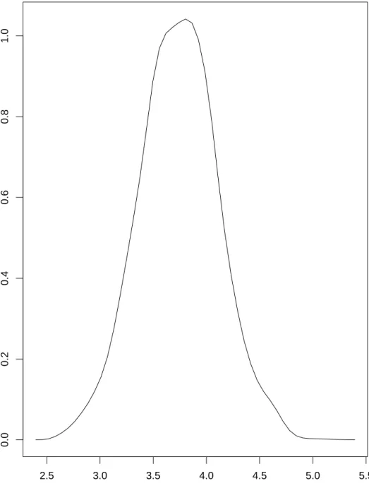
After theburn-inperiod, the frequency of appearance of the parameters in the Markov chain represents their posterior distribution. For example, Figure 2 displays the pos-terior density of the median return to education in 1991 obtained from our model (see supra). An informative full density distribution of the model parameters is read-ily obtained rather than a single point estimate as in a classical approach. Confi-dence/credible intervals are easily derived from the posterior distribution. Similarly, summary statistics, such as the posterior mean and the posterior standard deviation of the parameters, can also be computed in a straightforward manner from the distribu-tion.
Once the MCMC is successful, and the posterior probability distribution is sim-ulated, all summary statistics and confidence intervals for the conditional quantiles are computed very easily. This is particularly useful when we want to derive sum-mary statistics that are combinations of parameter estimates, such as a (marginal) return when a variable enters in quadratic form (see our experience variable in the application).1 Classical analysis would typically use a “plug-in” approach and combine
1If simultaneous quantile regression models were setup, Bayesian inference would provide
(condi-tional) percentile differences or percentile ratios easily; a feature that would be very appealing in income or wage distribution analysis. However, Bayesian inference for simultaneous quantile regression is not yet fully developed. This is a topic we are investigating elsewhere.
parameter estimates, but without necessarily taking the correlation of the estimates into consideration correctly. This poses no problem with Bayesian inference.
4
The wage return to education, experience and public
sector employment for British men
4.1 Data and empirical model
We illustrate application of Bayesian quantile regression with a classical Mincerian human capital earnings function of the form (Mincer, 1974):
ln(Yi) =φ(Xi) +i,
where ln(Yi) is the natural log of earnings or wages for individuali, Xi is a vector of individual characteristics reflecting the worker’s human capital (that usually includes a measure of educational attainment, a measure of the stock of accumulated experience, and other factors such as race, gender, ability measures, etc.). Classical quantile re-gression has been frequently applied to such models in recent years; see, among others, Buchinsky (1994), Machado and Mata (2002), or Nielsen and Rosholm (2002).
Our illustration is based on data about male British workers extracted from the British Household Panel Survey (BHPS). The BHPS is a longitudinal survey of private households in Great Britain covering a wide range of topics: income, employment, education, health, housing, etc. The initial survey was made in 1991 with interviews repeated annually thereafter. We use the first eleven waves of data covering the period 1991-2001. We only retain in our sample at each wave full-time male workers (excluding the self-employed). Sample sizes range from 1948 observations (wave 3, 1993) and 2275 observations (wave 1, 1991).
The response variable of interest, Yi, is the real gross hourly wage. For the sake of brevity, we limit the set of individual characteristics to education, experience (and experience squared), and a dummy variable indicating whether the person is working in the private or public sector. We use a standard log-linear formulation (Willis, 1986, Polachek and Siebert, 1993):
ln(Yi) =β0+β1Si+β2Ei+β3Ei2+β4Di+ui
whereSi is the number of years of schooling, Ei is potential experience (approximated by the age minus years of schooling minus 6), and Di is equal to 1 for public sector workers and 0 otherwise. This model follows closely Buchinsky’s (1994).
We estimate the quantile regressions using Bayesian inference at five quantile points, namely 0.10, 0.25, 0.50, 0.75 and 0.90, and for each of the eleven sample years available between 1991 and 2001. Independent improper uniform priors are used for all coefficients estimated. We simulated realizations from the posterior distribution of each parameter by means of the single-component Metropolis-Hastings algorithm described above. Each of the parameters was updated using a random-walk Metropolis algorithm with a Gaussian proposal density centered at the current state of the chain.
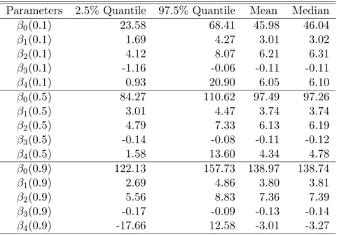
We discarded the first 1000 runs in every case and then collected a sample of 2000 values from the posterior of each of the coefficients. As an illustration, credible intervals for the parameters of each of the 0.1, 0.5 and 0.9 quantile regression parameters in the year 1991 are reported in Table 1. The table also shows the posterior mean and median. The reported numbers are the coefficients times 100. The first two columns represent 95% confidence intervals of the coefficients.
Table 1: Mean and median estimates and 95% intervals for the 0.1, 0.5 and 0.9 quantile regressions parameters for 1991
Parameters 2.5% Quantile 97.5% Quantile Mean Median β0(0.1) 23.58 68.41 45.98 46.04 β1(0.1) 1.69 4.27 3.01 3.02 β2(0.1) 4.12 8.07 6.21 6.31 β3(0.1) -1.16 -0.06 -0.11 -0.11 β4(0.1) 0.93 20.90 6.05 6.10 β0(0.5) 84.27 110.62 97.49 97.26 β1(0.5) 3.01 4.47 3.74 3.74 β2(0.5) 4.79 7.33 6.13 6.19 β3(0.5) -0.14 -0.08 -0.11 -0.12 β4(0.5) 1.58 13.60 4.34 4.78 β0(0.9) 122.13 157.73 138.97 138.74 β1(0.9) 2.69 4.86 3.80 3.81 β2(0.9) 5.56 8.83 7.36 7.39 β3(0.9) -0.17 -0.09 -0.13 -0.14 β4(0.9) -17.66 12.58 -3.01 -3.27 4.2 Return to education
The estimated returns of an additional year of education at the five quantiles are reported in Table 2. The reported numbers are the posterior means of the coefficients on education (β1) in the different regressions times 100. In parentheses are the posterior standard errors times 100. Table 2 also reports the mean return to education from a least square regression estimation. The posterior means are plotted in Figure 4.
Return to education differs across quantiles of the conditional wage distribution. Returns to education are higher at higher quantiles than at bottom quantiles. This indicates that the difference in the conditional wage distribution across education levels is not only characterized by a change in location, but also by an increase in spread. There is greater dispersion in the wages of highly educated workers. This would be completely missed by a mean regression. The best paid of highly educated workers do indeed benefit largely from their high education level, but education does not necessary ‘pay’ as much for all workers since the gradient at the lowest quantile is smaller. This is likely due to the heterogeneity of fields of specialization of educated workers, and different market value of different disciplines.
Table 2: Percentage return of an additional year of education, computed as the deriva-tive of the quantile regression with respect to education (evaluated at the posterior mean) times 100. The numbers in parentheses are standard errors.
Year mean 10%q 25%q 50%q 75%q 90%q 1991 3.69 3.01 3.56 3.74 3.93 3.80 (0.44) (0.26) (0.44) (0.36) (0.38) (0.24) 1992 3.97 2.81 3.65 4.10 4.12 4.37 (0.44) (0.27) (0.33) (0.43) (0.39) (0.33) 1993 4.09 3.47 4.01 4.30 4.25 4.14 (0.45) (0.32) (0.32) (0.44) (0.44) (0.30) 1994 4.27 2.94 4.02 4.37 4.60 4.92 (0.47) (0.26) (0.31) (0.28) (0.23) (0.35) 1995 4.03 2.92 3.61 3.96 4.26 4.67 (0.46) (0.37) (0.37) (0.25) (0.36) (0.45) 1996 3.76 3.23 3.72 3.92 4.32 4.59 (0.45) (0.22) (0.22) (0.22) (0.33) (0.33) 1997 4.08 2.98 3.73 4.33 4.34 4.46 (0.45) (0.35) (0.35) (0.47) (0.49) (0.34) 1998 4.01 3.15 3.67 3.94 4.09 4.40 (0.45) (0.46) (0.26) (0.49) (0.39) (0.48) 1999 4.06 2.86 3.44 4.16 4.33 4.60 (0.45) (0.47) (0.47) (0.26) (0.44) (0.48) 2000 4.31 3.29 3.47 4.18 4.67 4.86 (0.45) (0.37) (0.45) (0.26) (0.49) (0.36) 2001 4.26 3.20 3.77 4.28 4.60 4.81 (0.45) (0.43) (0.33) (0.36) (0.48) (0.36)
In general, Table 2 suggests that there has been an increase in the gap between high-pay and low-pay workers (conditionally on education) since return to education at the 0.1 quantile did not change much in the 1991-2001 period whereas return to education at the 0.9 quantile tended to increase (especially in the first half of the 1990s).
4.3 Return to experience
Experience enters in quadratic form in our model. The return to experience, i.e. the derivative of the conditional quantile of log wage with respect to experience, is therefore given by a combination of coefficients β2+ 2β3×Experience, where the coefficientsβ2 andβ3correspond to the coefficients on experience and experience squared respectively. The derivative needs to be evaluated at some specified level of experience. Two points were chosen: 5 years of experience, representing fairly new entrants, and 15 years of experience, representing experienced workers. The results are reported in Table 3 for the new entrants and in Table 4 for experienced workers. The reported number in the tables are the estimated returns of an additional year of experience times 100.
Table 3: Percentage return to an additional year of experience (at 5 years of experience)
Year mean 10%q 25%q 50%q 75%q 90%q 1991 5.99 5.74 5.34 5.56 6.05 8.03 (0.44) (0.34) (0.43) (0.56) (0.45) (0.35) 1992 5.44 5.0 4.84 5.05 5.59 6.16 (0.43) (0.30) (0.48) (0.51) (0.45) (0.37) 1993 5.75 5.46 5.44 5.54 6.0 6.68 (0.35) (0.38) (0.35) (0.36) (0.39) (0.22) 1994 5.40 5.24 5.11 5.33 5.87 6.01 (0.47) (0.34) (0.43) (0.56) (0.45) (0.35) 1995 6.00 5.27 5.58 5.69 6.05 6.16 (0.46) (0.30) (0.48) (0.51) (0.45) (0.37) 1996 5.88 5.55 5.12 5.78 6.08 6.61 (0.45) (0.38) (0.35) (0.36) (0.39) (0.22) 1997 5.25 5.30 5.22 5.64 6.15 6.58 (0.44) (0.49) (0.49) (0.44) (0.47) (0.36) 1998 5.75 6.0 5.35 5.60 6.22 6.82 (0.45) (0.22) (0.24) (0.26) (0.25) (0.24) 1999 5.60 5.00 4.68 5.41 5.72 6.00 (0.45) (0.48) (0.44) (0.36) (0.31) (0.23) 2000 5.60 5.07 4.77 5.52 6.02 5.81 (0.45) (0.32) (0.43) (0.63) (0.27) (0.25) 2001 5.12 4.17 4.52 5.17 5.66 6.00 (0.45) (0.32) (0.43) (0.63) (0.27) (0.25)
The larger values of Table 3 compared to those of Table 4 indicate that the return to experience tapers off with accumulated experience. For the younger workers, an
Table 4: Percentage return to an additional year of experience (at 15 years of experi-ence) Year mean 10%q 25%q 50%q 75%q 90%q 1991 4.79 4.59 4.26 4.42 5.82 4.34 (0.44) (0.47) (0.25) (0.30) (0.27) (0.38) 1992 4.44 3.97 3.90 4.06 4.47 4.96 (0.43) (0.48) (0.29) (0.29) (0.32) (0.54) 1993 4.65 4.36 4.39 4.46 4.79 5.35 (0.45) (0.52) (0.35) (0.36) (0.39) (0.49) 1994 4.40 4.12 4.13 4.31 4.71 4.85 (0.47) (0.47) (0.25) (0.30) (0.27) (0.38) 1995 4.80 4.10 4.44 4.52 4.84 5.02 (0.46) (0.48) (0.29) (0.29) (0.32) (0.54) 1996 4.75 4.35 4.15 4.65 4.92 5.40 (0.46) (0.52) (0.35) (0.36) (0.39) (0.49) 1997 4.78 4.19 4.19 4.57 4.96 5.33 (0.45) (0.54) (0.38) (0.34) (0.33) (0.61) 1998 4.55 3.96 4.26 4.50 4.50 5.47 (0.45) (0.86) (0.37) (0.42) (0.42) (0.85) 1999 4.50 3.87 3.73 4.31 4.59 4.83 (0.45) (0.54) (0.41) (0.33) (0.41) (0.68) 2000 4.40 4.00 3.79 4.38 4.79 4.65 (0.45) (0.55) (0.35) (0.40) (0.34) (0.73) 2001 4.12 3.28 3.60 4.13 4.52 4.79 (0.45) (0.46) (0.36) (0.41) (0.24) (0.43)
additional year of experience is associated with a higher return than an additional year of education. For workers at 15 years of experience, an additional year of experience has an effect of similar magnitude to the effect of education.
Interestingly, the impact of experience on the conditional wage distribution is very different from the impact of education. Experience appears to contribute to a catch-up of low pay workers since it is higher at the 0.1 quantile than at the 0.25 quantile or at the median. Experience is more profitable to low-pay workers. However, there is less heterogeneity in the return to experience at different quantiles than in the return to education. This suggests that there is not as much heterogeneity in the gains from experience in the conditional wage distribution. The change in location is important with experience, but the change in spread is not as marked as with education.
4.4 Return to public sector employment
It is often reported among academics that, at identical skill levels, people, particularly male workers, can earn more by working in the private sector rather than in the public sector.2 However, Allington and Morgan (2003) pointed out that a recent Audit Com-mission survey (2002) of public sector employees identified ‘better pay’ as the single most significant factor that persuades them to remain in the public sector.
Our results shed light on this apparent paradox. Table 5 reports the percentage return to working in the public sector compared to working in the private sector, that is the estimates of model parameterβ4 times 100.
Mean regression indicates that the mean return to working in the public sector is positive: average wage rate is higher among public sector workers. But the striking result is that the effect of public sector employment varies largely across quantiles. It is large and positive at lower quantiles (above 10 percent for the 0.1 quantile). It is still generally positive at the median. But it is negative at the 0.9 quantile. The wage distribution is much more compressed among public sector workers: low wages (i.e. at the lowest decile) are higher in the public sector, whereas high wages (i.e. at the highest decile) are lower in the public sector compared to the private sector. So, on average, public sector workers are better paid than private sector workers, but at the same time, the chances of obtaining a high pay are higher in the private sector: a high-wage employee in the public sector may be able to get a better pay in the private sector (provided he remains at the upper decile of the conditional wage distribution in the private sector).
Note that there is a marked decreasing trend in the return to public sector employ-ment over the 1991-2001 period, except for the 0.1 quantile. The difference between top wages in the private sector and top wages in the public sector has increased sub-stantially. Return to public sector employment is turning negative at the 0.75 quantile in the second half of the period.
This analysis of the effect of public sector employment clearly illustrates that
look-2See Allington and Morgan (2003) and the recent AUT (Association of University Teachers in UK)
Table 5: Percentage return to public sector employment Year mean 10%q 25%q 50%q 75%q 90%q 1991 3.46 6.05 7.85 4.34 2.36 -3.02 (0.44) (0.49) (0.38) (0.39) (0.44) (0.37) 1992 6.80 14.19 10.81 7.61 4.30 -4.22 (0.44) (0.38) (0.47) (0.36) (0.39) (0.23) 1993 4.89 11.40 10.09 7.71 1.43 -3.73 (0.45) (0.34) (0.47) (0.46) (0.52) (0.56) 1994 5.27 19.26 12.08 7.78 0.76 -2.59 (0.47) (0.49) (0.56) (0.65) (0.48) (0.78) 1995 5.70 13.19 13.50 10.74 0.24 -6.24 (0.46) (0.49) (0.67) (0.55) (0.65) (0.68) 1996 5.37 13.57 12.69 9.36 1.69 -4.38 (0.46) (0.29) (0.64) (0.41) (0.56) (0.49) 1997 4.26 12.17 9.71 7.70 -.20 -6.39 (0.45) (0.59) (0.36) (0.46) (0.36) (0.49) 1998 1.24 11.04 7.29 3.39 -4.2 -8.38 (0.45) (0.52) (0.38) (0.47) (0.47) (0.41) 1999 -0.89 7.07 4.80 2.49 -5.28 -10.68 (0.45) (0.31) (0.58) (0.36) (0.46) (0.50) 2000 0.25 12.99 10.03 1.77 -5.42 -11.83 (0.45) (0.41) (0.37) (0.36) (0.46) (0.40) 2001 0.25 13.18 7.83 -1.21 -6.00 -11.66 (0.45) (0.41) (0.47) (0.66) (0.56) (0.40)
ing only at the mean regression would miss much of rich details of the private/public sector differences in pay.
5
Conclusion
Quantile regression methods are valuable tools in many fields of economics. As our application shows, they allow analysts to extract much richer information than with standard mean regression. This is particularly useful in income and wage distribution analysis.
We illustrate the applicability of Bayesian inference for quantile regression as an al-ternative to the classical frequentist methods. Based on a simple MCMC algorithm, the methods are relatively straightforward to implement and, unlike frequentist approaches to quantile regression, do not rely on estimation or approximation of the asymptotic variances of the estimated parameters. They may also provide estimation and fore-casts for parameters, and combination thereof, which fully take into account parameter uncertainty.
Our application to the wage distribution among male workers in the 1990s Britain based on eleven years of data extracted from the British Household Panel Survey reveals for example that education is associated with higher wages, but also with greater wage dispersion. The opposite shows up for experience which benefits more to low pay workers. But the most striking result is that the wage differential between private and public sector employees is poorly characterized by a difference in average wage only. The wage distribution among public sector employees is much more compressed. Therefore, if wages are, on average, higher in the public sector, high-wage workers receive a better pay in the private sector. This gap between high-pay public sector employees and high-pay private sector employees has been increasing markedly during the 1990s.
Acknowledgements
The present research has been (co-)funded by a grant of the European Commission under the ‘Transnational Access to major Research Infrastructures’ contract HPRI-CT-2001-00128 hosted by IRISS-C/I at CEPS/INSTEAD (Luxembourg). The BHPS data were made available through the ESRC Data Archive. The data were originally collected by the ESRC Research Centre on Microsocial Change at the University of Essex (now incorporated within the Institute for Social and Economic Research). Nei-ther the original collectors of the data nor the Archive bear any responsibility for the analyses or interpretations presented here.
References
Allington, N. and Morgan, P. (2003) Does it pay to work in the public sector? Evidence from three decades of econometric analyses, Public Money and Management, Oct., 253–262.
Bilias, Y., Chen, S. and Ying, Z. (2000) Simple Resampling Methods for Censored Regression Quantiles,Journal of Econometrics,99(2), 373–386.
Buchinsky, M. (1994) Changes in the US Wage Structure 1963-1987: Application of Quantile Regression, Econometrica,62, 405-459
Dickens, R. and Manning, A. (2002) Has the National Minimum Wage reduced UK wage inequality? Centre for Economic Performance Working paper 533, London School of Economics and Political Science, UK.
Disney, R. and Gosling, A. (1998) Does it pay to work in the public sector? Fiscal Studies,19, 347–374.
Koenker, R. and Bassett, G. W. (1982) Robust tests for heteroscedasticity based on regression quantiles,Econometrica,50, 43–61.
Machado, J. A. F. and Mata, J. (2002) Earning functions in Portugal 1982–1994: Evi-dence from quantile regression,Economic applications of quantile regression Edited by Fitzenberger, B., Koenker, R. and Machado, J. A. F., Physica-Verlag, 115–134.
Mincer, J. (1974)Schooling, Experience and Earnings. New York: The Natural Bureau of Economic Research.
Nielsen, H. S. and Rosholm, M. (2002) The public-private sector wage gap in Zambia in the 1990s: A quantile regression approach,Economic applications of quantile regression
Edited by Fitzenberger, B., Koenker, R. and Machado, J. A. F., Physica-Verlag, 169– 182.
Polachek, S. and Siebert, W. S. (1993) The Economics of Earnings, Cambridge, New York and Melbourne: Cambridge University Press.
Willis, R.J. (1986) Wage determinants, a survey and reinterpretation of human capital earnings functions, In Orley Ashenfelter and Richard Layard (eds.)The Handbook of Labor Economics, Vol. 1, Amsterdam: North Holland-Elsevier Science Publishers; 525–602.
Yu, K., Lu, Z. and Stander, J. (2003) Quantile regression: applications and current research area,The Statistican,52,331–350.
Yu, K. and Moyeed, R. A. (2001) Bayesian quantile regression,Statistics and Probability Letters,54, 437–447.
Iteration number beta_0 0 1000 2000 3000 4000 5000 0 246 Iteration number beta_1 0 1000 2000 3000 4000 5000 -0.05 0.0 0.05 0.10 Iteration number beta_2 0 1000 2000 3000 4000 5000 -0.02 0.02 0.06 Iteration number beta_3 0 1000 2000 3000 4000 5000 -0.0020 -0.0010 0.0 Iteration number beta_4 0 1000 2000 3000 4000 5000 0.0 0.5 1.0 1.5
Fig. 1. Time series plot of five model parameters based on 5000 iterations from Metropolis algorithm.
2.5 3.0 3.5 4.0 4.5 5.0 5.5 0.0 0.2 0.4 0.6 0.8 1.0
The views expressed in this paper are those of the author(s) and do not necessarily reflect views of CEPS/INSTEAD.
Please refer to this document as