Agent based modelling of the dry bulk shipping sector

(1)

Agent Based Modelling of the Dry Bulk Shipping

Sector

Eoin Jude O’Keeffe

PhD Thesis

UCL

November, 2018

(2)

Signed Declaration

I, Eoin O’Keeffe confirm that the work presented in this thesis is my own. Where information has been derived from other sources, I confirm that this has been indicated in the thesis.

(3)

Abstract

This thesis presents an agent based model of the dry bulk shipping sector. The model is highly disaggregated, representing all voyages and cargoes transported through to 2050, including approximately 500 shippers and 750 shipowners with a total fleet of greater than 1000 vessels. In multiple projection scenarios, 2700 trade flows are modelled. The purpose of the approach is to identify a high fidelity representation of the system to gain a greater understanding of how aggregate level properties, for example total fuel

consumption, are generated from individual company based decisions such as when to transport cargo, what vessels to use, and what technology to invest in. Contracts of affreightment, the spot market and time charter market are represented within the model to create, where possible, a realistic representation of actual contractual conditions. The model is deployed to investigate the impact of climate change on the sector. Specifically, it investigated: physical impacts of climate change through the opening of Arctic sea routes; changing demand for commodities due to climate change and projected evolution of the global economy; changing fuel prices due to external projected changes in the shipping sector, and; effects of mitigation of climate change through carbon pricing and minimum standards on vessel efficiency. A key finding from the work is that endogeneous changes in the shipping system, through for example shipper preferences, create greater variability than those driven by external factors. This variability is reflected in the number of vessels in each of the size categories, the technology uptaken and the strategic approach of shippers in transporting their cargo. There remains a strong coupling of transport supply and emissions, with the regulations tested and available technology not resulting in significant improvements in energy efficiency. On the modelling of the dry bulk shipping system, clear computational and scope limits were identified. On

computational limits, the system is constrained such that parallelisation is limited leading to long runtimes. To understand the effects of agents choices, the modelling of the individual voyages is necessary leading to large degrees of freedom. In addition, the work has highlighted the need for more validation data of greater granularity.

(4)

Impact Statement

This work provides a platform for further work and analysis on the dry bulk shipping sector and more generally on the shipping sector as a whole. The model is developed to be easily extended so that further work both in academia and commercially can be applied. It has a number of applications but particularly its main goals are policy testing and operational research for commercial value. The model links the more abstract higher level approaches of scenario modelling at the global scale with company level operations to allow businesses understand how their decisions impact and are impacted by the wider policy environment and, vice versa, how policy impacts are manifested at the company scale.

The model allows the physical impacts of climate change to be simulated to understand how these can effect the commercial environment. The modelling approach adopted is not restricted to those impacts tested within the thesis. The model platform can easily be extended, for example, to allow a dynamic trade model to be included so that feedbacks between the shipping system and trade can be understood better.

The model allows users to view the shipping sector in a more interactive way that goes beyond significantly abstracted representations of the sector. A typical criticism that businesses have of model representations of their sectors is that they are too complex and too abstracted. The approach in this thesis and the model generated allows shippers and shipowners to implement policies that they would directly use with very little abstraction. It therefore goes some way to bridging the gap between academic modelling and business practical problems.

(5)

Acknowledgements

I have spent a number of years working on this thesis. Throughout that time I’ve received an incredible amount of support from lots of people, far too many to mention them all here. But there are some I must mention. My wife, Michelle, has provided amazing support throughout this process. If she knew how long this would have gone on for, I’m sure she would have added ”til the the 1000th conversation about agents and networks do us part” to our wedding vows. However, if she did I would never have been able to finish it without her. More recently, Lochie, my one year old son, has given me invaluable insights into the behaviour of a random agent. Having Lochie around has also given me the urgency to finish this work so I can spend more time with him and less time with agents.

Mark, my principal supervisor, despite my incredible lateness at submitting the thesis has provided unflinching support and whose knowledge of modelling has been invaluable. Tristans boundless knowledge about the shipping industry and his continuous support has also been indispensable.

Simon Davies has been incredibly helpful in talking through aspects of the shipping industry and imparting his wider business knowledge. More generally, he has provided encouragement and support both in my work at MATRANS and on this work.

Richard Scott was incredibly kind to give up so much of his time to discuss the dry bulk shipping sector with me on so many occasions. His insights into the business realities of the sector were both interesting and invaluable.

George Danner very kindly gave up his time while over in the UK to discuss my approach and subsequently was profligate with his time on skype.

When I was about to give up on on my code altogether and instead try to simulate the behaviour of the shipping system through the medium of dance, Rob McBryde

provided help towards the end to help me get the model over the line. Without him, I would still be trying to debug memory leaks!

(6)

(7)

List of Figures

6.1 Analysis Approach . . . 51

6.2 PHD Timeline . . . 52

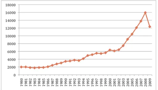
8.1 Global merchandise exports . . . 55

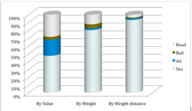
8.2 Modal split for world exports . . . 58

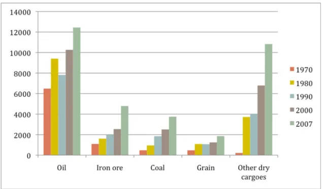
8.3 World seaborne trade in ton-miles for bulk commodities . . . 60

8.4 Major crude oil exporters . . . 61

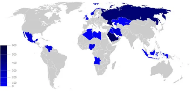
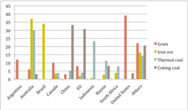
8.5 Selected world bulk commodity exporters . . . 62

8.6 The trajectories of all cargo ships . . . 64

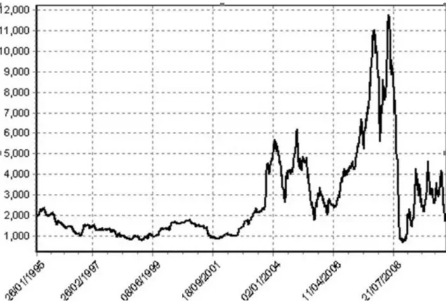
8.7 Baltic Exchange Dry Index . . . 70

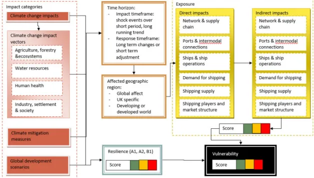
8.8 Schematic view of methodology . . . 71

8.9 Regional distribution of four climate-sensitive health consequences . . . . 76

8.10 Interlinking Pathways . . . 80

8.11 Mapping Vulnerability . . . 81

8.12 Vulnerability Scores . . . 98

8.13 Overall Results . . . 99

8.14 Combined results of vulnerability to climate change impacts. . . 100

8.15 Combined results of vulnerability to climate change mitigation. . . 100

(16)

8.17 Hurricane locations . . . 104

8.18 Water security risk index . . . 105

8.19 Multi-model mean of annual mean surface warming . . . 106

9.1 Global imports of dry bulk commodities . . . 108

9.2 Time series of grouped commodities as trade demand and prices . . . 110

9.3 Percentage of total trade (t) in each commodity . . . 111

9.4 Time series of all commodity flows . . . 112

9.5 Port database comparisions . . . 115

9.6 Location of ports in selected ports database. . . 116

9.7 The number of ports in each country in Europe with a designated maxsize 116 9.8 European ports split by max size . . . 117

9.9 DBSS Fleet size distribution . . . 118

9.10 The Baltic Dry Index . . . 120

9.11 Trip charters versus voyage charters . . . 121

9.12 Time charters for capesize vessels . . . 122

9.13 Vessel delivery and demolitions . . . 124

9.14 Drybulk shipyards . . . 125

9.15 Secondhand vessel market . . . 126

9.16 Economic Order Quantity model . . . 130

9.17 Economic order quantity model . . . 131

9.18 Factors influencing agreed spot price . . . 133

(17)

10.4 Spot Market, genetic algorithm formulation . . . 145

10.5 Exemplar pricing problem for two vessels inGooFy . . . 146

10.6 Process for time chartering the vessel withinGooFy. . . 148

10.7 Formulation for selecting time charter vessel . . . 149

10.8 Process for CoA chartering withinGooFy . . . 150

10.9 Formulation vessel selection genetic algorithm . . . 151

10.10Commodity flow process modelling . . . 154

10.11Brownian demand . . . 154

10.12Independence of port combinations . . . 155

11.1 Maritime inventory routing problem (MIRP) as a basic formulation . . . . 161

11.2 Formulation of the FSM shipping problem . . . 162

11.3 Basic formulation of the maritime fleet sizing problem (MFSP) . . . 163

11.4 MIRP formulation in discrete time for a single product . . . 165

11.5 SRPTP formulation . . . 166

11.6 Shipper operational planning routing problem . . . 167

11.7 Shipowner operational planning routing problem . . . 168

11.8 Rational Expectations . . . 171

11.9 Shipper fleet sizing (FSM) . . . 172

11.10Risk based shipper strategy . . . 173

11.11Pure play (industrial) shipper strategy . . . 175

11.12Pure Play (CoA) shipper strategy . . . 176

11.13Pure play industrial shipper strategy . . . 177

11.14Setting the operational cargo size . . . 178

11.15Setting the operational cargo size . . . 180

(18)

11.17Risk averse operational strategy for setting the number of cargoes to ship 181

11.18Risk averse and Responsive Shipper operational strategy for setting offer

price for cargoes . . . 182

11.19FSM shipowner strategy. . . 184

11.20Random strategic planning for shipowner . . . 185

11.21Pure play spotmarket Shipowner strategy . . . 186

11.22Pure play spotmarket Shipowner strategy (cont’d) . . . 187

11.23Shipowner tactical planning . . . 188

11.24Responsive strategy for tactical planning for shipowner . . . 188

11.25Random strategy for tactical planning for shipowner . . . 189

11.26Estimation of reserve price . . . 190

11.27Shipowner operational planning responsive . . . 191

11.28Shipowner operational placing cargoes on spot . . . 191

11.29Shipowner operational planning reposition . . . 192

11.30Shipowner operational planning random . . . 192

11.31Formulation for selecting time charter vessel . . . 193

12.1 Volume transported by run . . . 203

12.2 Number of vessels and tonnage for each scenario . . . 205

12.3 Number of vessels scrapped each year in each scenario and run . . . 205

12.4 Number and tonnage of vessels built in each year . . . 206

12.5 The number of vessels in each size category . . . 207

12.6 Transport work in each size category . . . 208

(19)

12.10Vessel count and cargo asks for Run 1 . . . 212

12.11Vessel count and cargo asks for Run 2 . . . 213

12.12Vessel count and cargo asks for run 3 . . . 214

12.13Vessel count and cargo asks for run 4 . . . 215

12.14Degree and node strength for ports . . . 216

12.15Mean operational speeds in each size category in all runs . . . 217

12.16The plots show the number of shipper schedules on each of spot, industrial and CoA . . . 218

12.17Days at sea for each size category . . . 219

12.18Total annual fuel consumption . . . 220

12.19Mean operational efficiency index . . . 221

12.20Actual fixtures prices with $/tekm estimated . . . 222

12.21Model time series plots of spot prices . . . 223

12.22Model time series plot of mean spot price . . . 224

12.23Model time series plot of mean time charter price . . . 225

12.24Model time series plot of mean CoA rate . . . 225

13.1 Data generating process for commodity prices . . . 228

13.2 Commodity price in each scenario . . . 229

13.3 The effect of truncating the trade to a selected number of countries . . . . 230

13.4 Template for generating shortest paths for capesize vessels . . . 232

13.5 The three carbon price scenarios used inGooFy . . . 233

13.6 The three fuel price scenarios used inGooFy . . . 234

13.7 Reported monthly grain exports from the USA . . . 236

13.8 GDP, coal energy and biomass energy growth rates used inGooFy . . . 237

13.9 Technology options with associated MEPC reference. Source: Smith et al. (2010) . . . 240

(20)

13.10List of scenarios that are run inGooFy . . . 242

14.1 Annual cargo delivered in each scenario . . . 244

14.2 Time series of number of vessels in each size category . . . 245

14.3 Time series of spot market price in each size category . . . 247

14.4 Annual emissions ofCO2for all vessels . . . 249

14.5 Fuel consumption in each scenario. . . 250

14.6 Time series vessels built and scrapped . . . 251

14.7 Technical Efficiency across all runs . . . 251

14.8 Top 5 technologies installed in size 0 for each run in 2050 . . . 252

14.9 Top 5 technologies installed in size 0 for each run in 2020 . . . 252

14.10Top 5 technologies installed in size 2 for each run in 2050 . . . 253

14.11Top 5 technologies installed in size 2 for each run in 2020 . . . 253

14.12Operational efficiency index across all runs . . . 254

14.13Transport work in scenarios for SSP1 . . . 256

14.14Transport work in scenarios for SSP5 . . . 257

14.15Final year transport work in each commodity for SSP1 . . . 258

14.16Final year transport work in each commodity for SSP5 . . . 259

14.17Number of vessels in each size category for each of the policy scenarios and trade scenarios . . . 261

14.18Port degree. . . 262

14.19Mean operational speed of vessels in each size category for each of the policy scenarios and trade scenarios. . . 263

(21)

14.24The amount of trade carried by each schedule type in each scenario . . . . 268

14.25Spot prices and Lomb-Scargle Periodogram for these spot prices . . . 269

14.26Vessels built and scrapped and Lomb-Scargle Periodogram for these values 270

14.27Example vessel network for a random vessel . . . 270

(22)

List of Tables

2.1 Glossary of Abbreviations . . . 26

2.2 Glossary of terms . . . 27

2.3 Typical categorical/discrete objects as used within equations . . . 28

2.4 Amended Strategy definition symbols . . . 28

2.5 Superscript definition used in agent strategies . . . 28

2.6 Continuous variables . . . 28

2.7 Matching casing and notation to traditional notation use. . . 29

2.8 Symbol glossary for commodity production and consumption . . . 29

2.9 Symbol glossary for trade . . . 30

2.10 Symbol glossary for ship operations and route network calculations . . . . 30

2.11 Symbol glossary for ship technology and efficiency . . . 30

2.12 Symbol glossary subscripts used in equations . . . 30

2.13 Symbol glossary for operation, tactical and strategic models . . . 31

8.1 Summary of climate change projections . . . 74

(23)

Chapter 0 LIST OF TABLES

12.1 Scenario names run for the validation hindcasting . . . 201

12.2 Shipper Types . . . 201

12.3 Shipowner types . . . 201

12.4 Criteria for mix scenarios for shipper agent . . . 202

12.5 Criteria for mix scenarios for shipowner agent . . . 202

12.6 Vessel size labels used in theGooFyscenarios . . . 207 13.1 Scenario Regulation . . . 232

13.2 Growth rate categories for each commodity . . . 236

13.3 Cargo parcel size categories . . . 238

13.4 Typical additional vessel costs . . . 239

13.5 Criteria for mix scenarios for shipper agent . . . 241

13.6 Criteria for mix scenarios for shipowner agent . . . 241

14.1 Vessel size ranges . . . 244

(24)

Chapter 1

Part A: Context

1.1

Thesis Outline

The thesis is divided into two sections. After a glossary introduction,Part Abegins by outlining the research questions and then provides an introduction to challenges within the industry in the context of climate change with a specific focus on the dry bulk shipping sector (DBSS). This introduction provides a context to the research questions provided in the earlier chapter.Part Bprovides the framework for the thesis and modelling along with results and conclusions.

InPart A,Chapter 4andChapter 5provide an introduction to complex adaptive systems and their applicability to the modelling of the shipping sector. They also provide some analysis of existing approaches to modelling transport in the long run within the maritime field. InPart B,Chapter 7which provides an outline of the

approach used in the thesis. Next a background and context for the analysis is provided through a qualitative risk assessment of the shipping industry inChapter 8followed by a more indepth analysis of the DBSS in the proceeding chapter. An agent based model is described in detail inChapters 10and11with associated verification and validation in Chapter 12. The scenarios used in this study are described inChapter 13and their associated results focussed on the research questions inChapter 14.

(25)

Chapter 2

Glossary and Formatting

2.1

Introduction

The following chapter outlines the abbreviations and terms used throughout this thesis. The terms are first introduced in the text in long format and thereafter used in their abbreviated form. Additionally, there is provided an outline of the approach used in model symbols and terms in later chapters.

The formatting used in this thesis follows the rules below:

• References to chapters, sections, figures and tables occur inBoldwith first letter capitalised

• Abbreviations and terms occur in normal text

• References to the model on which the thesis is based,GooFy, and the agents and objects withinGooFyoccur initalics. In the chapters that deal with the structure of

GooFy, this can result in words, such as shipper, occuring in bothitalicsand normal font. When it occurs in normal font, it refers to the object in the real world rather than how it is manifested withinGooFy(GooFyis not an acronym).

(26)

Chapter 2 2.2. Glossary of Abbreviations and terms

Abbr Full name

ABM Agent Based Modelling

ACE Agent Based Computational Economics AIS Automatic Identification System

BDI Belief-Desire-Intention BDI Baltic Dry Index BFI Baltic Freight Index

CAS Complex Adaptive Systems CIF Cost, Insurance & Freight CoA Contract of Affreightment CN Competing Nations scenario CRP Cargo Routing Problem DBSS Dry Bulk Shipping Sector DWT Deadweight Tonnage EBM Equation Based Modelling ECA Emission Control Area

EEDI Energy Efficiency Design Index EEOI Energy Efficiency Operational Index EMF Efficient Market Hypothesis

EOQ Economic Order Quantity ETS Emissions Trading Scheme FSM Four Stage Modelling FSM Fleet size and mix problem

GA Genetic Algorithm

GC Global Commons scenario

GHG Greenhouse Gas

IMO International Maritime Organisation LDT Vessel Light displacement

MABS Multi-Agent Based Systems MAC Marginal Abatement Cost

MEPC Marine Environment Policy Committee MIRP Maritime Inventory Routing Problem SEEMP Ship Energy Efficiency Management Plan SQ Status Quo scenario

SRPTP Ship routing problem of tramp shipping SSP1/SSP5 Shared Socio-Economic Pathways 1 and 5

(27)

Chapter 2 2.3. Model Symbols Glossary

Term Description

Agribulks Agricultural goods transported in the bulk sector typically grains, soya, fertiliser.

Cabotage Coastal shipping transport within a country Capesize Dry bulk vessels typically greater than 200,000t

Deadweight Typical indicator of the size of a vessel, representing its cargo carrying capacity in tonnes

Dry bulk

shipping

Dry cargoes that are large enough for vessel loads, eg. coal, iron ore and grain.

Layup This is when a vessel is anchored in a sheltered location for a period of time with no crew (or at least minimal for safety) and does not engage in market activities

Layday The day of arrival that a vessel must be at a load port to collect cargo Parcel size Refers to the volume of cargo transported

Panamax Largest category of vessels that can traverse the Panama canal. In this thesis, it is designated as 60,000 to 100,000t

Pure play Referring to a company that focusses on a particular market segment Retrofit The physical alteration of an active vessel that, typically, improves its

fuel efficiency

Shuttle service Cargoes are delivered by a vessel that transits from load port to discharge in a round trip without diverting to other ports

Suezmax Largest category of vessel that can traverse the Suez canal. In this thesis, it is designation at 100,000 to 200,00 t

Valemax Maximum size vessels as commissioned by the Brazilian mining company Vale. These were later termed Chinamaxes

Wet bulk

shipping

Liquid bulk cargoes such as chemicals, oil and petroleum products

Table 2.2. Glossary of terms

2.3

Model Symbols Glossary

2.3.1 Models for Agent strategies

Categorical and continuous variables can be superscripted to a subset. These subsets are shown as uppercase, for exampeCF IXED orCF indicates fixed vessels costs.

(28)

Name Set symbol Indexing symbols

Commodity flow between ports for a shipper K k

Commodity c c Vessel V i, j Routes Rv r Vessel Type V v Count of vessels Y v, i Binary indicator X i, x Profit π i Revenue R v, i Time Consumed Z v, r

Table 2.3. Typical categorical/discrete objects as used within equations

For agent strategies that have been deployed inGooFy, the symbols used in the model definitions change, particularly in the broader use of other terms such as production and consumption.

Name Set symbol Indexing symbols Capacity or Demand Q t, r

Table 2.4. This table shows agent strategy definition symbols that have either changed or are not covered inTable 2.3

Name Superscript Example Applications Days at sea DAY S AT SEA TDAY S AT SEA

Days in port DAY S IN P ORT TDAY S IN P ORT

Production P ROD QP ROD_rt

Table 2.5. Superscript definition used in agent strategies

Name units Set symbol Indexing symbols Example superscripts

rate NA d i, j RISK,W ACC

Speed km/hr S i LOW

(29)

2.3.2 Other

The notation for superscripts when referencing agents is based on a simple camel casing principle. The first letter of each word within the variable is captialised and used in the variable names with an additional letter appended if this does not create a unique variable or for further descriptive purposes. Each subscript defines association of the variable to an instance of a particular entity with superscripts providing additional information about the variable such as association to an entity type. For example,C_iShis total costs to shipper i, whileC_iSodefines total costs to shipowner i. By utilising the superscripts for additional definition, it allows reuse of subscript letters. Each additional entity is separated by a comma, for example,T C_i,kShmeans the total costs to shipper i for commodity k. Note that commodity is not a superscript as k is only used to denote commodity. Similarly, c is only used to denote cargo. In the example above, the first superscriptShis matched with the first subscriptimeaning shipper i. However, since there is no associated superscript with k, it exists independently.

Where possible variables in equations are shown in lower case. The following correspondence table is used for comparison.

This thesis Typical usage Description

Pi pi Price of item to owneri. This could also be a vector of pricesP P Matrix of all prices and all owners.

Table 2.7. Matching casing and notation to traditional notation use.

Outputs from models will also be assigned to X and Y variables. These are used as matching variables (often binary).

Name Symbol Definition Units

Crop yield CY Crop yield per km2of land, typically

calculated for each country te/km2 Factor inputs X Quantity of factor inputs. Typically

subscripted with L for land, C for capital, and

lb for labour km2/$/numbers

Price p International price of commodity $/te Production Q Quantity of commodity produced

(typically in a country) te

(30)

Name Symbol Definition Units

Balancing Factors A, B Used for the calculation of the O-D matrix

Exports O Commodity quantity for export from a country te Generalized transport T C Monetised cost of transport $ cost

Imports D Demand of a commodity of a country. te

Table 2.9. Symbol glossary for trade

Name Symbol Definition Units

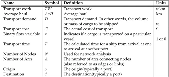
Transport work T W Transport work tekm

Average haul AvH Average haul km

Transport demand D Transport demand. In other words, the volume or mass of cargo to be shipped te Transport cost C The actual cost of transport $ Binary flow variable x Indicates if a cargo is transported on a particular

vessel 1 or 0

Transport time T The calculated time for a ship from arrival at one to arrival at another port

Number of Nodes N Used for network analysis

Number of Arcs A The number of arcs connecting nodes (also referred to as edges or links) Origin o The origin(typically a port) Destination d The destination(typically a port)

Table 2.10. Symbol glossary for ship operations and route network calculations

Name Symbol Definition Units

Fuel Intensity F I

Specific fuel constant sf c Factor to convert tonnes of fuel to tonnes of CO2

Emissions Em CO2Emissions te

Table 2.11. Symbol glossary for ship technology and efficiency

Symbol Referring to

i, j Agent

m, n Location

v Vessel. E.g. Route network optimisation

c Cargo.

k Commodity

(31)

Symbol Referring to

bid Bid price offered by shipper for transport of cargo

ask Ask price of shipowner for hiring their vessel

Q Annual volume on route

q Cargo parcel size

(32)

Chapter 3

Research Question and hypotheses

3.1

Research Question and Hypotheses

This thesis seeks to outline that mitigation in the DBSS must be considered in the context of climate change and adaptation. It does this by investigating the effects, both direct and indirect, of climate change on the DBSS through to 2050. Additionally, this thesis proposes the use of highly disaggregated simulation modelling, in the form of ABM, as being a suitable tool to investigate these impacts. These will be investigated through the hypotheses:

1. The treatment of the dry bulk shipping sector as a system of heterogeneous agents allows modelling of complex behaviour not captured with existing approaches in the field.

2. Setting shipowners and shippers as learning agents creates different take up of technology as compared with treatment of these entities as having consistent homogeneous market preferences.

Hypothesis 1seeks to show that the system behaviour should not be constrained to an equilibrium type approach where supply is matched to demand on an annual basis. In fact decisions are made on an individual company basis at a point in time, where the decision is influenced by prevailing market conditions and the expected future conditions from the perspective of that company.Hypothesis 2seeks to show that by

(33)

Chapter 3 3.2. Brief Elucidation

In addition to dealing with the hypotheses above, the following research questions are to be investigated:

1. Will climate change impacts be similar across the route network, as the opening of new northern routes only affects certain commodities and trades?

2. Will relative changes in demand for dry bulk commodities, potentially as a result of climate mitigation policy in other sectors, lead to significant changes in the world shipping system such as arrangement of the world fleet structure?

3. Will the impact of climate change mitigation regulations cause a change in the provision of transport thus reducing the uptake of carbon emission reducing technologies?

3.2

Brief Elucidation

Research question 1) looks specifically at the cascading effect of changes to a specific route. For example, the opening of a new shorter route may effect the economic order quantity for a trade, by reducing the gains from economies of scale. The reduction in demand for this vessel size may change the overall demand for vessels of this size. This could lead to changes in parcel size for other trades that would have been shipped in this vessel size, as the overall liquidity in this size range is reduced.

Research question 2) deals particularly with climate policy sensitivity of commodities, with a focus on coal demand. It investigates whether the change in demand will simply reduce the demand on those vessels that would have supplied this transport or, as alluded to above, whether there are cascading impacts that will affect demand in other size ranges.

Research question 3) investigates the negative feedbacks from climate change policy. Will the adoption of a price of carbon have unintended consequences.

Tesfatsion (2006) outlined four areas of understanding in ABM:

1. Empirical Understanding: Can observed global regularities be generated in an ABM simulation?

2. Normative understanding: Can we generate good economic designs for the system, for example through policy intervention?

3. Qualitative insight and theory generation: Can we gain greater understanding of the real system through a systematic examination of their dynamical behaviours?

(34)

Chapter 3 3.2. Brief Elucidation

4. Methodological advancement: Can we improve approaches in ABM?

This research focuses on 1), 2) and 3). The approach looks to gain a normative

understanding focussed on the double externality problem, where the private return is not matched by the social return (Faber & Frenken 2009), and market barriers to take up of emissions reducing technology in the context of climate change.

(35)

Chapter 4

Introduction

4.1

Maritime transport and the global economy

Globalisation has transformed the world in the last fifty years. Over this period, the growth in trade has allowed increasing choice for many countries, often being

responsible for improvements in health and welfare. As a result, trade is often perceived as the backbone of globalization, allowing goods to be produced and shipped in the most efficient manner to allow consumers access at their lowest price. The reduction in transport cost has been facilitated through technological innovations and has occurred at a time when there has been increased trade liberalization (Tamiotti et al. 2009).

The freight shipping sector’s value lies in its ability to service global trade. The importance of the sector is borne out in the fact that growth in world GDP has been historically correlated with growth in seaborne merchandise tradeUNCTAD (2009), albeit reducing in strength in recent years Constantinescu et al. (2015), Mangan (2017). This historical coupling is something particularly apparent in the economic expansion of developed countries. Consequently, when we consider impacts on the shipping sector, it is important to consider these in terms of their key interfaces with the global economy. More specifically, the cost and reliability of transport supply and externalities, such as air pollution and greenhouse gas (GHG) emissions , are not currently accounted for in these costs (with some limited exceptions)

The transport of goods, particularly long distance transport, is dominated by shipping. Indeed, the greatest contribution of shipping to global trade has been to make sea transport so cheap that the cost of freight for non time-dependent products is in many cases negligible when considering where to source goods. This is the major reason why shipping dominates the transport of goods and this cost performance has been achieved by a combination of economies of scale, new technology, better ports, more efficient

(36)

Chapter 4 4.1. Maritime transport and the global economy

cargo handling and the use of international flags to reduce overheads (Stopford 2009).

Indeed, some authors predicted a ”death of distance” as transport costs became lower and lower. However, Carrere & Schiff (2004) found the opposite to be the case with distance of trade declining for most countries with elements such as regional integration and counter-season trade and their relative evolution to be important, and indeed distance remains a key determinant of trade (Disdier & Head 2008, Williams & Gr´egoire 2015). This suggests that the system is complex making it difficult difficult to extract simple causal relationships from aggregated data.

The importance of transport costs in trade is less to do with their absolute value but rather the transport cost relative to the total value of the good (Korinek & Sourdin 2009). For high value goods, such as apparel, this could be between 2-4% for maritime

transported goods but for low value commodities such as iron ore it could be as high as 60% (Korinek & Sourdin 2009). Thus the importance of transport cost for low value goods (wetbulk and drybulk in particular) is crucial. As alluded to above, distance is often found not to be a good proxy for trade patterns (Martinez-Zarzoso &

Nowak-Lehmann 2007). There is some discussion that time to market is a better proxy for transport costs than distance (Korinek & Sourdin 2009), but it is likely only to be the case for containerised cargoes particularly retail goods such as apparel. In many cases, particularly in the dry bulk sector, the transit time is less important than service reliability. In fact, there is surprisingly little detailed information available on

micro-level trade flows to help gain greater understanding of the transport of goods.

As Anderson & Van Wincoop (2004) outline, transport costs vary by country to country pairing and indeed by commodity. Moreover, there can also be significant intra annual variation in these prices, as some commodities, particularly agribulks (such as grains and fertiliser), are seasonal in production. There is also tension between commodities that have substitutable transport. For example, coal and iron-ore both are transported on capesize (200,000t+ vessels), thus relative demand is important in determining transport cost as it is supply sensitive.

When considering long run projections of the shipping sector, it is important to fully understand how issues such as cost and service reliability can change. Cost is fundamentally dependant on the voyage cost, the demand and the supply. In an oversupplied market, transport costs move toward voyage costs: the marginal cost of transport. As demand increases above supply, the voyage cost becomes a lower bound and the price becomes dependent on the shippers willingness to pay (and ship operators willingness to offer transport at that time). Although pricing at an aggregate level is

(37)

Chapter 4 4.2. Maritime hazards: Past and future

4.2

Maritime hazards: Past and future

The global system of maritime trade is a complex dynamic system. The derived demand for shipping is considered as the volume of cargo for transport factored by the distance over which it needs to be transported, meaning both aggregate demand and trade pattern are important. Superimposed on this are time variations due to seasonal availability and demand, short-term cycles (both endogeneously and exogeneously generated), economic cycles and long term trends.

The key drivers of fluctuations in the sector have been due to temporal, geographical and commodity inconsistencies in matching supply and demand. Vessels have a

lifespan of 25 to 30 years, while demand for transport, as alluded to above, adjusts over much shorter timescales. Together with this, short term fluctuations in the cost of transport are often due to mismatching of demand location and supply location. Many vessels, particularly larger bulk vessels, spend almost half their sailing time carrying no cargo (in ballast) as they must relocate to areas where there is demand. The option of vessel substitution is also limited as many commodities are restricted by their state (liquid, gas, solid), cargo size (supply chain requirements lacking flexibility) and market related demands.

Coupled with these existing challenges, future developments include greater demand from Asia and developing countries as well as significant changes in commodities being transported having dramatic effects in the dry and wet trades. Additionally, climate change potentially will have significant direct and indirect impacts, and as such can be considered to be a ”threat multiplier”. For example, localised weather conditions can cause crop failures which in turn alters demand and supply within a region that in turn causes volatility in transport demand for that crop. In addition, due to the long life of vessels, climate change mitigation policies enacted now (or not) will have lasting effects on the maritime sectors ability to deal with changing physical climate conditions.

Together with possible impacts, the maritime sector must also cut its emissions significantly as part of a global effort to avoid dangerous climate change (Smith et al. 2014). Therefore, determining the most effective path at reducing emissions whilst avoiding increased exposure to systemic risks is important for the welfare of the industry.

As alluded to above, the shipping sector consists of several distinct sub-sectors, most notably dry (e.g. grains and iron ore), wet (e.g. oil and chemicals) and containerised. These are distinct due their product properties. Containerised trade is typically run on scheduled services so it can transport less than vessel load cargoes. Dry and wet typically carry a single cargo, and for larger vessel sizes, this involves a single drop-off. Although some vessels exist that can service more than one of these sub-sectors, they are

(38)

Chapter 4 4.3. Maritime transport modelling paradigm and its limitations

dominated by specialised vessels that service a single sector. AlthoughChapter 8 provides a sector wide assessment, the focus of this thesis is on the DBSS. As with containerised and wet, it is typically considered a distinct market and thus a hard system boundary assumed from a vessel allocation perspective. Secondly, it transports low cost cargo and is thus sensitive to changes in transport cost. Thirdly, it is a

significant proportion, in mass, of the cargo transported globally and therefore significant alterations in this system would have a material affect on sector wide

emissions. Finally, it carries cargo that is sensitive to climate change impacts and climate change mitigation policies, and thus allows consideration of feedbacks from climate effects.

4.3

Maritime transport modelling paradigm and its limitations

The focus in this section is on approaches that model sector-wide changes in the long run. Transport modelling of this kind is largely based on the four stage modelling (FSM) paradigm. The FSM has been adopted in regional and global models following their extensive use in passenger modelling (Ortuzar & Willumsen 2001). These are, largely, equilibrium type models, although there are many different implementations. FSM adopts the principal that trade and transport can effectively be split into four separate categories for ease of modelling:

• Trip generation: The total number of trips originating from a node are estimated.

• Trip distribution: The destinations of the trips are estimated to form an origin-destination matrix.

• Modal split: The share of modes are calculated for each origin/destination pair.

• Trip assignment: The origin/destination demand for each mode is assigned to a route.

FSMs were developed in the passenger transport sector and were adopted by freight transport modellers. Macro-level models using this FSM approach, such as STREAMS, VACLAV, SAMSGODS and TRANS-TOOLS for the European area (Kraft et al. 2010, Bergkvist et al. 2005), measure the effects of control polices. These use coarse-grained data either at the national level or disagregated to sub-national regions (typically NUT3/2 zones) resulting in up to 1300 traffic cells. It should be noted that these models

(39)

Chapter 4 4.3. Maritime transport modelling paradigm and its limitations

As noted by Bergkvist et al. (2005), many of these models fail to account for logistical processes and as a result fail to model at the level where the decisions regarding the actual transports are taking place. For minor changes, this may be sufficient but for large infrastructural alterations or significant changes in transport costs identification and incorporation of feedbacks and other system responses is difficult. Furthermore, Bergkvist et al. (2005) suggest that micro-level models are best placed to capture the decision making of the actors in the logistical process.

For the most part (with some notable exceptions such as ASTRA), each individual step with the FSM consists of what Parunak et al. (1998) refer to as equation based modelling (EBM), where the model is a system of equations and execution consists of evaluating them. For geographical systems, EBM models are represented as static aggregations of populations, rational aggregated behaviour and flows of information (Crooks & Heppenstall 2012), effectively assuming homogeneity within the system. Solution approaches included multiple regression, location-allocation and spatial interaction models (Crooks & Heppenstall 2012). For transport this typically takes place within the FSM framework.

In particular, EBMs substitute what Tesfatsion (2006) called “equilibrium assumptions for procurement processes”. This is reasonable for systems that have a stable

equilibrium as procurement processes may not effect the long run state. Tesfatsion (2006) cites Fisher (1989)

The theory of value is not satisfactory without a description of the

adjustment processes that are applicable to the economy and of the way in which individual agents adjust to disequilibrium. In this sense, stability analysis is of far more than merely technical interest. It is the first step in the reformulation of the theory of value.

As Crooks & Heppenstall (2012) suggest, geographical systems are characterised by continual change and evolution through space and time with interactions between agents felt at different scales as well as over differing timescales. The limitations of EBM can be its assumption of equilibrium or steady state, which is an exception in the real world (Kraft et al. 2010).

As noted at the beginning of this chapter, the shipping system has radically changed over the last fifty years, therefore, as we look to project over that same magnitude of time the assumption that the system only undergoes minor perturbations is

questionable.

Existing approaches have struggled to explain phenomena within the shipping system in a useful way to increase resilience. Together with this, there is a necessity to unlock investment in new technology that will reduce emission of pollutants and GHGs. As is

(40)

Chapter 4 4.4. Research Focus

shown by marginal abatement cost (MAC) curves, there is enormous potential here but market barriers hinder this. Unlocking these, requires an understanding of the

environment in which they act at the company level.

There have been some notable exceptions to EBM within the FSM framework. Song et al. (2005) adopt a disagregated pipe-network approach to modelling the container shipping network. The transport demand and shipping are inputs to their model. As such it is serves as an assignment model in the FSM mould. Kraft et al. (2010) coupled a systems dynamics model with a static network based approach.

A number of other studies focussed on the shipping sector with the aim of projecting GHG emissions (as well as pollutants) within the sector (rather than, for instance, transport policy), most notably the GHG studies sponsored by the International Maritime Organisation (IMO). The most recent iteration, Smith et al. (2014), used a scenario based approach that assumed an exogeneous transport demand. The transport supply was estimated using assumed capacity utilisation factors. Fuel consumption and emissions were then estimated using an assumed evolution of fuel mix, technology, fuel and carbon costs. The performance of the fleet (in terms of fuel consumption and emissions) was derived from these assumed drivers by estimating cost driven technology take up (Smith et al. 2014).

4.4

Research Focus

The exigencies of climate change have spawned large areas of research both on the science and its associated economic and social effects. In the context of shipping, most research has been focused on reducing emissions from the sector through technological advances and operational optimisation. However, a holistic understanding of these risks is hampered by the lack of quality data available to researchers. Indeed, attempts to quantify emissions have led to large ranges of estimates from the sector. Thus most research has focused on clarifying this area to determine some base line value from which emissions trajectories can evolve.

Unfortunately, impacts of climate change on shipping and trade have been somewhat overlooked (Tamiotti et al. 2009, Watson & Wright 2010). This is particuarly concerning as according to a number of studies, not least Rogelj et al. (2011) and more recently Raftery et al. (2017), it is extremely likely we will exceed the 2 degree C above preindustrial levels target based on full implementation of current commitments.

(41)

Chapter 4 4.5. Summary

abatement cost curves (MAC curves) are often used to identify the technologies and changes that could be adopted to reduce emissions often at negative cost. However, MAC curves contain an inherent contradiction - negative cost technologies should already be implemented. Consequently, the use of these tools to identify barriers to uptake (only one of which is the direct monetary cost of implementation) can at best be complementary to a more sophisticated understanding of the system.

Some considerable work on predicting the transport demand in the sector in the long run and its expected emissions and technology uptake has been undertaken (for

example Smith et al. (2016) and Eyring (2005)). However, in many respects this provides little understanding in how the system will evolve. In this thesis, research focuses on the DBSS system, particularly treating the DBSS as a complex adaptive system and using the approach, agent based modelling (ABM), in analysing it.

As Bergkvist et al. (2005) state, EBM contain an enforced structure whereas in ABM the structure is emergent from the interactions between the individuals. Further to this, Parunak et al. (1998) states that

ABM is most appropriate for domains characterized by a high degree of localization and distribution and dominated by discrete decisions. EBM is most naturally applied to systems that can be modelled centrally, and in which the dynamics are dominated by physical laws rather than information processing.

4.5

Summary

Shipping dominates the transport of goods and commodities by volume, largely due to its economies of scale. Although the cost of transport is driven by distance and volume, the dynamics of geographic supply and demand, amongst other factors, result in large fluctuations in the price of transport in the short term with changing trade patterns and the long lifespan of vessels affecting it in the long term.

The modelling of the evolution of the shipping sector has predominantly followed the canonical transport modelling approach of the FSM and other equilibrium based approaches. These approaches are appropriate for systems that are, unlike the shipping industry, stable and not subject to constant supply-demand inequalities. This chapter introduced a more suitable approach: consideration of the system in terms of its interacting agents. In this situation, the aggregate supply-demand balance is an emergent property rather than an enforced boundary. Due to the distinction between the various sectors within the industry, each shipper sub-sector can be considered in isolation, with this thesis focussing on the DBSS. The main contribution of this thesis is

(42)

to propose a complex adaptive systems approach for understanding the maritime shipping system to understand how it can be expected to respond under different future scenarios.

(43)

Chapter 5

The Emergence of Complexity

5.1

Introduction

This chapter provides a brief introduction to complex adaptive systems with a particular focus on the modelling of those systems using ABM. Following this it provides some examples of applications of ABM in relevant fields before focussing on its applicability to the research. Finally, it discusses limitations of the approach.

5.2

Emergence of Complexity

A system is complex if it is composed of interacting units which exhibit emergent properties, becoming a complexadaptivesystem (CAS) when these interacting units exhibit goal-directed behaviour (Tesfatsion 2006). Moreover, CAS are a subset where the agents within the system can adapt locally to maximise their utility or fitness.

The study of CAS investigates how the interactions of the parts of the system give rise to collective behaviours of the system. Key elements of these complex systems are that the interactions between agents are typically local and non-linear. These local, rich

interactions lead to emergent behaviour at the macroscopic level. Together with this, complex systems have a historic dependency and most importantly operate far from equilibrium conditions. The assumption of equilibrium is a key to most EBM models that is relaxed in this framework. As discussed inChapter 4, there remain knowledge gaps of the causal mechanisms in the shipping system; the investigation of causal mechanisms of this type is a fundamental goal of agent based modelling (Tesfatsion 2006).

(44)

Chapter 5 5.2. Emergence of Complexity

approach and explicitly treat complexity within global systems and spawned the area of system dynamics. Specifically, it models the causal mechanisms and feedbacks of the system by treating the system as a series of rates and flows. The system is allowed to evolve, rather than producing point estimates at defined periods, without an enforced equilibrium or steady state. However, by not considering the individual agents interactions, it contains an enforced structure and is considered an EBM style

approach.Notwithstanding this limitation, ABM, and other fields such as complexity science, are related to this approach and draw on this and other fields for their theoretical foundations.

ABM tends to be referred to in different areas: Multi-Agent Based Systems (MABS) in flow systems and Agent Based Computational Economics (ACE) in business based applications. Although they diverge in naming convention, their framework and model structure is fundamentally the same. For this thesis, the convention of agent based modelling (ABM) is used.

Bonabeau (2002) succinctly outlines the advantages of ABM over other modelling techniques:

• ABM captures emergent phenomena: The whole is more than the sum of its parts where emergent system properties may seem counterintuitive to the properties of the parts. Therefore, it is good for finding system regularities that the user is interested in altering or at the very least understanding their provenance.

• ABM provides a natural description of a system: Describing a system using a series of aggregate analytical models is conceptually considerably more abstract than defining how agents interact with each other whether physically (eg. in traffic flows) or in marketplaces (eg. through bids and asks).

• ABM is flexible: It can be trivial to adjust the number of agents and more importantly vary their strategies and their complexity. For an EBM, this can require changes to the system structure (Van Dam 2009).

Macal & North (2010) suggest that CAS was originally motivated by investigations into adaptation and emergence of biological systems and has been said to have its origins in the evolutionary theory of Darwin. Chen (2012) suggests that ABM as applied in market simulation has its origin in work of Leon Walras’ 1874 proposal for a competitive

general equilibrium model. However, the major breakthrough which brought the approach into common use was in Thomas Schelling’s (Schelling 1969, 1971) models of

(45)

in 1996 (Epstein & Axtell 1996) that ABM was applied to entire artificial societies (Crooks & Heppenstall 2012) and began to be applied more widely.

Although definitions vary of an agent, Tesfatsion (2006) describes it as “bundled data and behavioural methods representing an entity constituting part of a computationally constructed world”. Examples range from individuals to firms and institutions as well as crops and livestock and physical entities such as geographical regions. Macal & North (2010) extends the agent definition to requiring certain characteristics:

• An agent is identifiable with decision-making ability.

• An agent is situated with the ability to recognise and distinguish the traits of other agents.

• An agent may be goal-directed, autonomous and self-directed. As Macal (2016) note, the approach takes ”the agent persepective”.

Agents were originally rule based but have since been embedded with the potential for learning and memory (Crooks & Heppenstall 2012). The development of learning in ABM, followed two paths: normative learning that described the optimal learning process and learning that causes behaviour to converge towards optimal behaviour in equilibrium (Brenner 2006). Different fields favoured different learning paradigms with macro-economists favouring normative approaches and evolutionary algorithms and genetic programming frequently used in ACE. Reinforcement learning in ACE models has been applied to a large extent through the three main models: Bush-Mosteller, the principle of melioration and the Roth-Erev model.

However, there remains strong links to the early modelling with agent depiction in many simulations remaining (near) zero-intelligence or indeed randomly behaving agents. For example, financial agents are often modelled as zero-intelligence agents because their strategic behaviours are poorly known and understood (Chen 2012). This work has grown alongside a paradigm shift in micro-economics, where traditional assumptions of rationality and homogeneity are being challenged (Macal & North 2010). This included developments in consumer theory on the concept of bounded rationality, where consumers cannot know the property of all goods due to capacity and

information constraints (Faber & Frenken 2009) and in behavioural economics such as the concept of satisficing (Simon 1996). Possibly the most important contribution from ABM, is its ability to generate complex phenomena or system regularities from a set of relatively simple agent rules (Luke et al. 2003).

An advantage of ABM is that the agents that are modelled can range from those with primitive reactive decision rules to complex adaptive artificial intelligence (Macal & North 2010). ABM has also facilitated the modelling of heterogeneity within agents,

(46)

where they not only differ in skills and knowledge but also in preferences (Faber & Frenken 2009, Abar et al. 2017).

The architectures on which ABM is developed have increased dramatically with a number of different software platforms available. Further to this Wooldridge & Jennings (1995), defined four agent types: logic based agents, reactive agents,

belief-desire-intention (BDI) agents and layered architectures; which define these

architectures. The design of the architectures is considered as important as the design of the ABM itself (Lang et al. 2008), with the framework creating the shared ontology through which the agents interact and the system evolves. These architectures or environments define the operational space of agents, meaning agents can be spatially explicit (a location in geometrical space) or implicit meaning their location is irrelevant (Crooks & Heppenstall 2012). For MABS, agent communication languages were developed as context-free grammars to allow complete flexibility within the

architecture, facilitating agent communication (Lang et al. 2008). The move towards these concepts of mental agency occurred in the 1990s in the BDI architecture.

The early 2000s saw a significant increase in the number of publications adopting an evolutionary perspective (Faber & Frenken 2009), dominated by ABM approaches. This trend has continued with ABM approaches been deployed in many disciplines

including economics, sociology, psychology, archaeology, language studies and management (Faber & Frenken 2009, Macal 2016, Moglia et al. 2017), and indeed, it continues to find new areas of deployment (Nicholls et al. 2017).

According to Macal & North (2010), ABM should be applied when long-run equilibrium states are not the only results of interest, and when the past is no predictor of the future. Furthermore, they suggest that the systems requiring understanding are becoming more complex if not always too complex for EBM approaches.

InChapter 4, the future impacts on shipping were introduced. These would suggest that the environment and demands on shipping are going to dramatically change over the coming years. A key factor that has been highlighted by many authors is the market barriers that exist in shipping to uptake of energy efficient technologies. Another key reason for using ABM is that agents learn and engage in dynamic strategic behaviour (Macal & North 2010). To understand the effect of, and ultimately to be able to remove, market barriers is a key research point.

More concretely, ABM facilitates a greater understanding of the system at work. There is a good understanding of each of the factors at work and how these can cause macro

(47)

Chapter 5 5.3. Applications of Agent Based Modelling

(Parunak et al. 1998). This mapping of interactions is naturally defined over networks or geographies.

5.3

Applications of Agent Based Modelling

A key area where ABM has achieved significant success is the area of innovation

diffusion modelling, a trend likely to continue Moglia et al. (2017). Until the application of ABM to this subject, most work in technological innovation focussed on the seminal contagion model by Bass (1969). Although still nascent, it has created interesting work by facilitating a transition from an aggregate-level to an individual-level perspective (Kiesling et al. 2012).

Geographic systems have seen a wide application of ABM to investigate geographical problems like urban sprawl (Crooks & Heppenstall 2012). For example, Heppenstall et al. (2006) modelled geographic retail markets.

The dominant work in ACE has been on auction systems or advances on Sugarscape (Epstein & Axtell 1996) in growing economies. Such work has also carried over to transportation marketplaces, for example Dai & Chen (2011) developed an ABM framework in a carrier collaboration problem. The profit allocation is determined following collaboration amongst carriers that is facilitated by an auction process. However within the transportation sector, ABM applications have focussed on optimisation approaches to traditional operational research problems and traffic problems. For example, Farhan (2015) developed a simulation model for capacity planning of a cross border facilty accounting for pedestrian flows.

MABS systems in particular have been deployed as decision support systems in the areas of vehicle routing and transportation firm engagement. These areas have typically seen the deployment of optimisation systems. As Lang et al. (2008) suggest, ABM has the ability to include negotiation and cooperation that optimisation based approaches do not. This has led Davidsson et al. (2005), amongst others, to conclude that ABM is the way forward for transport logistics, a prediction that has largely been borne out

(El-Amine et al. 2017).

Bergkvist et al. (2005) developed an ABM that can simulate a transport chain to understand the consequences of control policies in an operational setting (buying and selling of vehicles is not considered). The work itself was in an early phase, but showed the potential of such approaches in transport logistics. Engelen et al. (2009) completed one of the few ABM applications in the shipping sector. This approach is on short run analysis of the DBSS freight markets to assess the Efficient Market Hypothesis (EMF), concluding that bounded rationality is a suitable paradigm for DBSS agents.

(48)

Chapter 5 5.3. Applications of Agent Based Modelling

Furthermore, they suggest that shipping companies tend to use practical filter rules or rules of thumb when making tactical and strategic decisions. A conclusion of their work was that defining a market equilibrium as a result of interacting individual strategies is a powerful approach to describing market price patterns.

These are notable exceptions in the application of modelling paradigms within the shipping sector. Most focus has been on integration across agents with little work on representing the different planning stages that protagonists use within the DBSS. More concretely, the DBSS does not have the same challenges of integration that liner

shipping in particular has. The focus, to date, has been on determining the validity of assumed economic conditions and market properties such as the efficient market hypothesis (Engelen et al. 2009).

As highlighted by Bonabeau (2002), a key reason to use ABM is when agent interactions are heterogeneous and can generate network effects. Kaluza et al. (2010) showed that each of the main shipping subsectors resemble small world networks (Watts & Strogatz 1998) as well as other key emergent properties. Another reason, is that averages will not work (Bonabeau 2002): the shipping sector is strongly cyclical, but is treated as linearly stable in most approaches when in fact fluctuations are amplified within the system causing the cyclical phenomenon. As Stopford (2009) states, the sector is driven by cycles not long term trends.

As will be discussed inChapter 11, shipping stakeholder behaviour is complex and is difficult to capture through aggregate transition rates. Activities, such as the various planning levels, are a more natural way to describe these agents.

5.3.1 Limitations of Agent Based Modelling

As with all models, a general purpose model cannot work. This appears a greater issue with ABM, as there is the temptation to model all interactions and processes within the real system. As the focus is, typically, on emergent properties of the system, setting a system boundary before these have been identified is difficult. Hence, there is a focus on developing simple models and adding complexity. As reiterated by Bonabeau (2002), this process remains an art more than a science. Too much detail can lead to excessive constraints and become overly complicated. Too little and key feedbacks and

regularities may be missed. A key factor of CAS is its sensitivity to initial conditions. Given the level of detail required for defining an ABM system, the initial state of the system may not be completely known. Indeed, small changes in rules of interactions can

(49)

the computational demand. Parallelisation can be deployed, but only on systems where the agents can be separated into parallel processes - typically in a physical space based model such as the modelling of human civilisations. If a system requires that all agents are interacting, or at least it is non-trivial in decomposing the groups into sub-groups, such as through communication networks, then opportunities for parallelisation are limited. Although computational power is constantly increasing, it remains a strong limiting factor.

As visual and flexible tools, a typical benefit of ABM is that it is a tool that users can play with, what Crooks & Heppenstall (2012) refer to as a miniature laboratory. However, this is also cited as a limitation. As Bonabeau (2002) suggests, “a manager cannot claim to have saved $X million by playing with a simulation of her customers”. In this regard, it is is ideal to adopt different approaches to tackling the same problems. Therefore, the parallel use of an EBM with an ABM is not without merits.

The main limitation in ABM is the area of validation and verification (Crooks et al. 2008). This is discussed in greater detail inChapter 12when applied to the model developed in this work. Faber & Frenken (2009) refer to this limitation euphemistically as a “problematic relationship”. The validation process is an assessment of the “extent to which the model is a good representation of the process that generated a set of

observ