The Roles of Language Models and Hierarchical Models in Neural Sequence-to-Sequence Prediction

The Roles of Language Models and

Hierarchical Models in Neural

Sequence-to-Sequence Prediction

Felix Stahlberg

Supervisor:

Prof. Bill Byrne

Advisor: Prof. Phil Woodland

Department of Engineering

University of Cambridge

This dissertation is submitted for the degree of

Doctor of Philosophy

Declaration

I hereby declare that except where specific reference is made to the work of others, the contents of this dissertation are original and have not been submitted in whole or in part for consideration for any other degree or qualification in this, or any other university. This dissertation is my own work and contains nothing which is the outcome of work done in collaboration with others, except as specified in the text and Acknowledgements. This dissertation contains fewer than 65,000 words including appendices, bibliography, footnotes, tables and equations and has fewer than 150 figures.

Felix Stahlberg September 2019

Acknowledgements

According to the academic code of conduct it is imperative to acknowledge my supervisor, Prof. Bill Byrne. Since acknowledging one’s supervisor with flowery language is such a common thing to do, I find it difficult to sufficiently express my sincere and deep gratitude towards Bill in this context. There is no question that our many and long discussions were not only very enjoyable but also made me a much better researcher. Bill mastered the fine balance between guidance and freedom for me perfectly, giving me enough space and trust for pursuing my own (sometimes abstruse) research ideas while staying engaged to identify connections to other lines of research and alternative ways to go forward. Bill also taught me the value of formal rigorousness, and ensured that I have access to all the resources I needed for conducting and communicating my research – whether financial or computational.

I am also thankful to my co-authors Danielle Saunders from the Cambridge University, and Gonzalo Iglesias, Eva Hasler, and Adrià de Gispert from SDL Research. The scope of my PhD studies would have been much more limited without these fruitful collaborations. This thesis also draws from my two research internships – one at Google NY and one in the AML machine translation group at Facebook. I thank both teams for making me feel welcome, especially my hosts Brian Roark (Google), Richard Sproat (Google), and James Cross (Facebook).

On a personal note, I would like to thank my wife, Barbara Stahlberg, for her love, and con-stant support and encouragement. I also thank the Šepi´c family for (now officially) welcoming me in their midst last year, and Aarón Sanchez for always looking over my shoulder.

I was financially supported by the U.K. Engineering and Physical Sciences Research Council (EPSRC grant EP/L027623/1). Some of my work has been performed using resources provided by the Cambridge Tier-2 system operated by the University of Cambridge Research Computing Service1funded by EPSRC Tier-2 capital grant EP/P020259/1. I hope that, despite shifting political tides in the U.K., the research council will be able to continue to open doors for European students like it did for me.

Abstract

With the advent of deep learning, research in many areas of machine learning is converging towards the same set of methods and models. For example, long short-term memory networks are not only popular for various tasks in natural language processing (NLP) such as speech recognition, machine translation, handwriting recognition, syntactic parsing, etc., but they are also applicable to seemingly unrelated fields such as robot control, time series prediction, and bioinformatics. Recent advances in contextual word embeddings like BERT boast with achieving state-of-the-art results on 11 NLP tasks with the same model. Before deep learning, a speech recognizer and a syntactic parser used to have little in common as systems were much more tailored towards the task at hand.

At the core of this development is the tendency to view each task as yet another data mapping problem, neglecting the particular characteristics and (soft) requirements tasks often have in practice. This often goes along with a sharp break of deep learning methods with previous research in the specific area. This work can be understood as an antithesis to this paradigm. We show how traditional symbolic statistical machine translation models can still improve neural machine translation (NMT) while reducing the risk for common pathologies of NMT such as hallucinations and neologisms. Other external symbolic models such as spell checkers and morphology databases help neural grammatical error correction. We also focus on language models that often do not play a role in vanilla end-to-end approaches and apply them in different ways to word reordering, grammatical error correction, low-resource NMT, and document-level NMT. Finally, we demonstrate the benefit of hierarchical models in sequence-to-sequence prediction. Hand-engineered covering grammars are effective in preventing catastrophic errors in neural text normalization systems. Our operation sequence model for interpretable NMT represents translation as a series of actions that modify the translation state, and can also be seen as derivation in a formal grammar.

Table of contents

List of figures xvii

List of tables xxiii

Nomenclature xxix

1 Introduction 1

1.1 Motivation . . . 1

1.2 Contributions . . . 3

1.3 Organization of this Thesis . . . 5

1.4 Notations . . . 5

2 Statistical Machine Translation and Symbolic Models 7 2.1 Motivation . . . 7

2.2 N-gram Language Models . . . 8

2.3 Word-based Models . . . 8

2.4 Word Alignments . . . 9

2.5 Phrase-based Translation . . . 10

2.6 Weighted Finite State Transducers . . . 11

2.6.1 Formalisms . . . 12

2.6.2 Operations on WFSTs . . . 14

2.7 Hierarchical Phrase-based Machine Translation . . . 15

2.7.1 Synchronous Grammars . . . 15

2.7.2 FST-based Hierarchical Translation . . . 16

2.8 Conclusion . . . 17

3 Neural Machine Translation 19 3.1 Motivation . . . 19

xii Table of contents

3.2 Word Embeddings . . . 20

3.3 Phrase Embeddings . . . 21

3.4 Sentence Embeddings . . . 22

3.5 Encoder-Decoder Networks with Fixed Length Encodings . . . 23

3.6 Attentional Encoder-Decoder Networks . . . 26

3.6.1 Attention . . . 26

3.6.2 Attention Masks and Padding . . . 29

3.6.3 Recurrent Neural Machine Translation . . . 30

3.6.4 Convolutional Neural Machine Translation . . . 32

3.6.5 Self-attention-based Neural Machine Translation . . . 35

3.6.6 Comparison of the Fundamental Architectures . . . 37

3.7 Neural Machine Translation Decoding . . . 39

3.7.1 The Search Problem in NMT . . . 39

3.7.2 Greedy and Beam Search . . . 39

3.7.3 Formal Description of Decoding for the RNNsearch Model . . . 40

3.7.4 Ensembling . . . 42

3.7.5 Decoding Direction . . . 44

3.7.6 Efficiency . . . 45

3.7.7 Generating Diverse Translations . . . 46

3.7.8 Simultaneous Translation . . . 47

3.8 Open Vocabulary Neural Machine Translation . . . 48

3.8.1 Using Large Output Vocabularies . . . 48

3.8.2 Character-based NMT . . . 50

3.8.3 Subword-unit-based NMT . . . 52

3.8.4 Words, Subwords, or Characters? . . . 54

3.9 Using Monolingual Training Data . . . 55

3.10 NMT Model Errors . . . 57

3.10.1 Sentence Length . . . 57

3.11 NMT Training . . . 61

3.11.1 Cross-entropy Training . . . 62

3.11.2 Training Deep Architectures . . . 64

3.11.3 Regularization . . . 64

3.11.4 Large Batch Training . . . 66

3.11.5 Reinforcement Learning . . . 67

3.11.6 Dual Supervised Learning . . . 68

Table of contents xiii

3.12 Explainable Neural Machine Translation . . . 69

3.12.1 Post-hoc Interpretability . . . 69

3.12.2 Model-intrinsic Interpretability . . . 69

3.12.3 Confidence Estimation in Translation . . . 70

3.12.4 Word Alignment in Neural Machine Translation . . . 70

3.13 Alternative NMT Architectures . . . 71

3.13.1 Extensions to the Transformer Architecture . . . 71

3.13.2 Advanced Attention Models . . . 72

3.13.3 Memory-augmented Neural Networks . . . 73

3.13.4 Beyond Encoder-decoder Networks . . . 74

3.14 Data Sparsity . . . 75 3.14.1 Corpus Filtering . . . 75 3.14.2 Domain Adaptation . . . 76 3.14.3 Low-resource NMT . . . 77 3.14.4 Unsupervised NMT . . . 77 3.15 Multilingual NMT . . . 78 3.16 NMT Model Size . . . 79

3.17 NMT with Extended Context . . . 80

3.17.1 Multimodal NMT . . . 80

3.17.2 Tree-based NMT . . . 80

3.17.3 NMT with Graph Structures as Input . . . 81

3.17.4 Document-level Translation . . . 82

3.18 Conclusion . . . 82

4 SMT-NMT Hybrid Systems 85 4.1 Motivation . . . 85

4.2 Related Work . . . 86

4.3 Syntactically Guided Neural Machine Translation . . . 88

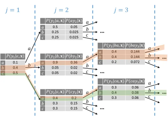
4.3.1 Hiero Predictive Posteriors . . . 90

4.3.2 FST-based Constrained NMT Decoding . . . 91

4.3.3 Experiments . . . 92

4.4 UCAM@WMT16: Combination Via Edit Distance Transducer . . . 97

4.4.1 The Edit Distance Transducer . . . 98

4.4.2 Loose Coupling of Hiero and NMT . . . 98

4.4.3 Experiments . . . 102

4.5 MBR-based Hybrid Machine Translation . . . 105

xiv Table of contents

4.5.2 Left-to-right Decoding . . . 107

4.5.3 Efficientn-gram Posterior Calculation . . . 107

4.5.4 Relation to MBR Decoding . . . 108

4.5.5 Subword-level MBR . . . 108

4.5.6 Experiments . . . 109

4.6 UCAM@WMT18: MBR-based System Combination of Multiple Models . . 112

4.6.1 Multiple System Combination . . . 112

4.6.2 System Setup . . . 114

4.6.3 Results . . . 118

4.7 Conclusion . . . 120

5 SGNMT – A Flexible NMT Decoding Platform 123 5.1 Motivation . . . 123

5.2 NMT Toolkits . . . 124

5.3 Predictors . . . 126

5.3.1 Example Predictor Constellations . . . 130

5.3.2 Predictor Wrappers . . . 131

5.4 Decoders . . . 132

5.4.1 Neural Decoding as Shortest Path Search . . . 134

5.4.2 NMT Batch Decoding . . . 138

5.4.3 Exact Inference in NMT . . . 139

5.4.4 Using Exact Inference to Characterize NMT Search Errors and Model Errors . . . 141

5.5 Output Formats . . . 146

5.6 Tuning Predictor Weights . . . 146

5.7 Applications . . . 148

5.7.1 SGNMT for Research . . . 148

5.7.2 SGNMT for Teaching . . . 149

5.7.3 SGNMT in the Industry . . . 150

5.8 Conclusion . . . 150

6 Unfolding and Shrinking Neural Machine Translation Ensembles 151 6.1 Motivation . . . 151

6.2 Unfolding Ensembles into a Single Large Neural Network . . . 153

6.3 Shrinking the Unfolded Network . . . 155

6.3.1 Data-Free Neuron Removal . . . 155

Table of contents xv

6.3.3 Shrinking Embedding Layers with SVD . . . 159

6.4 Results . . . 159

6.5 Probabilistic Interpretation of Data-Free and Data-Bound Shrinking . . . 164

6.6 Conclusion . . . 166

7 The Role of Language Models in Neural Sequence-to-Sequence Prediction 169 7.1 Motivation . . . 169

7.2 Neural Word Reordering Using Language Models . . . 170

7.2.1 Bag-to-sequence Modeling with Attentional Neural Networks . . . . 170

7.2.2 Search . . . 172

7.2.3 Results . . . 172

7.3 Neural Grammatical Error Correction Using FSTs . . . 174

7.3.1 Constructing the Hypothesis Space . . . 175

7.3.2 Experiments . . . 179

7.3.3 UCAM@BEA19: FST-based GEC in Shared Task Submissions . . . 182

7.4 Simple Fusion: Using Language Models for NMT Training . . . 185

7.4.1 Translation Model Training under Language Model Predictions . . . 186

7.4.2 Experimental Setup . . . 187

7.4.3 Results . . . 189

7.4.4 Discussion and Analysis . . . 189

7.5 UCAM@WMT19: Document-level Language Models for Translation . . . . 195

7.5.1 Document-level Language Modelling . . . 195

7.5.2 Results . . . 197

7.6 Conclusion . . . 200

8 The Role of Hierarchical Models in Neural Sequence-to-Sequence Prediction 201 8.1 Motivation . . . 201

8.2 Syntax-based NMT with Multi-representation Ensembles . . . 202

8.3 Neural Text Normalization Under Covering Grammars . . . 204

8.3.1 Neural Text Normalization Models . . . 205

8.3.2 Unconstrained Neural Text Normalization . . . 209

8.3.3 Constraining Neural Text Normalization with Covering Grammars . . 211

8.4 Operation Sequence Neural Machine Translation . . . 214

8.4.1 A Neural Operation Sequence Model . . . 215

8.4.2 OSNMT Represents Alignments . . . 216

8.4.3 OSNMT Represents Hierarchical Structure . . . 218

xvi Table of contents 8.4.5 Training . . . 222 8.4.6 Results . . . 222 8.4.7 Related Work . . . 229 8.4.8 Future Work . . . 230 8.5 Conclusion . . . 230 9 Conclusion 231 9.1 Language Models . . . 231 9.2 Hierarchical Models . . . 233 9.3 Implementations . . . 233 9.4 Final Remarks . . . 234 References 235

Appendix A List of Publications 299

Index 303

List of figures

2.1 Word alignment from the English sentence “What’s this used for” to the Spanish sentence “para que se usa esto”. . . 9

2.2 Generative story of IBM-3. . . 9

3.1 Number of papers mentioning “neural machine translation” per year according Google Scholar. . . 20

3.2 Recursive autoencoder followingSocher et al.(2011). The color coding indi-cates weight sharing. . . 22

3.3 The convolutional sentence model (Kalchbrenner and Blunsom,2013). The color coding indicates weight sharing. . . 22

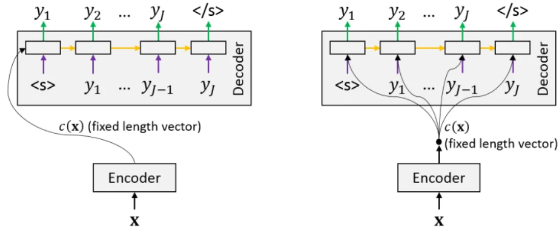
3.4 Encoder-decoder architectures with fixed-length sentence encodings. The color coding indicates weight sharing. . . 24

3.5 The encoder-decoder architecture ofSutskever et al.(2014). The color coding indicates weight sharing. . . 25

3.6 Encoder architectures. The color coding indicates weight sharing. . . 25

3.7 Attention weight matrixAfor the translation from the English sentence “history is a great teacher .” to the German sentence “die Geschichte ist ein großer Lehrer .”. Dark shades of blue indicate high attention weights. . . 28

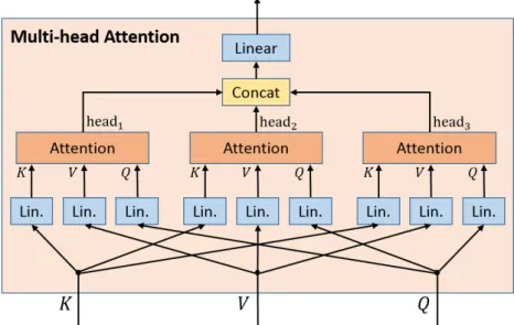
3.8 Multi-head attention with three attention heads. . . 28

3.9 A tensor containing a batch of three source sentences of different lengths (“the first cold shower”, “even the monkey seems to want”, “a little coat of straw” – a haiku by Basho (Basho and Reichhold,2013)). Short sentences are padded with <pad>. The training loss and attention masks are visualized with green (enabled) and red (disabled) background. . . 29

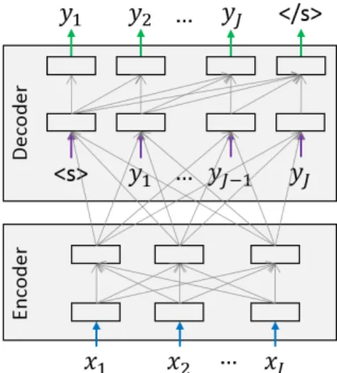
3.10 The RNNsearch model followingBahdanau et al.(2015). The color coding indicates weight sharing. Gray arrows represent attention. . . 30

xviii List of figures

3.12 Types of 1D-convolution used in NMT. The color coding indicates weight sharing. . . 33

3.13 NMT with a convolutional encoder and a convolutional decoder like in the ConvS2S architecture (Gehring et al., 2017b). The color coding indicates weight sharing. Gray arrows represent attention. . . 34

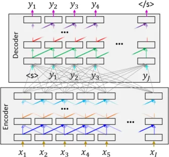
3.14 Purely attention-based NMT as proposed byVaswani et al.(2017) with two layers. The color coding indicates weight sharing. Gray arrows represent attention. . . 35

3.15 Comparison of NMT architectures. The three inputs to attention modules are (from left to right): keys (K), values (V), and queries (Q) as in Fig.3.8. . . 38

3.16 Comparison between greedy (highlighted in green) and beam search (high-lighted in orange) with beam size 2. . . 40

3.17 Ensembling four NMT models. . . 42

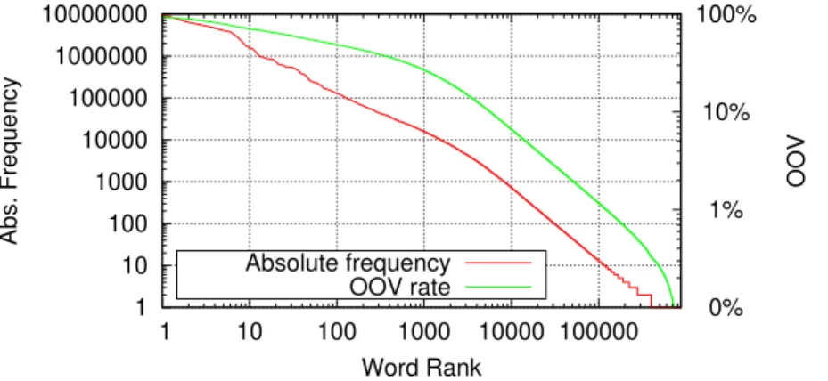
3.18 Distribution of words in the English portion of the English-German WMT18 training set (5.9M sentences, 140M words). . . 49

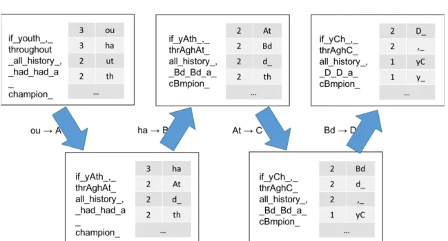
3.19 First four merge operations of the byte pair encoding (BPE) algorithm on the text “if youth, throughout all history, had had a champion” (the opening phrase of the 260 page novelGadsbyfrom EV Wright which deliberately contains only words without the letter ‘E’). Counts indicate the frequency of symbol bigrams in the text. . . 53

3.20 Hierarchical representation of the merge operations in the example in Fig.3.19. 53

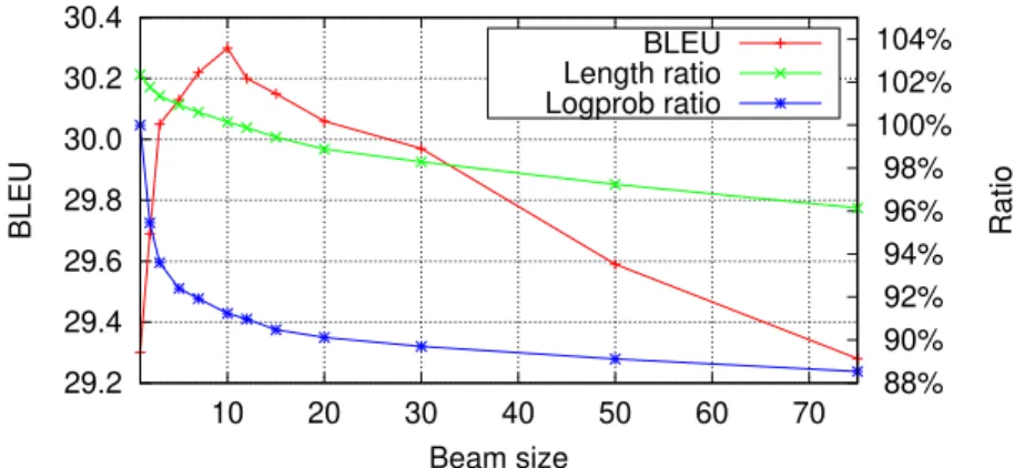
3.21 Performance of a Transformer model on English-German (WMT15) under varying beam sizes. The BLEU score peaks at beam size 10, but then suffers from a length ratio (hypothesis length / reference length) below 1. The log-probabilities are shown as a ratio with respect to greedy decoding. . . 58

3.22 The length deficiency in NMT translating the English source sentence “Her husband is a former Tory councillor.” into German following Murray and Chiang(2018). The NMT model assigns a better score to the short translation “Ihr Mann ist ein ehemaliger Stadtrat.” than to the greedy translation “Ihr Mann ist ein ehemaliger Stadtrat der Tory.” even though it misses the former affiliation of the husband with the Tory Party. . . 59

3.23 Neural networks with external memory. . . 73

4.1 Update of the decoder hidden state in standard NMT and syntactically guided NMT. Context vectors and recursive connections are omitted in this figure for the sake of simplicity. Layers are annotated with their dimensionality in a standard RNNsearch setup. . . 89

List of figures xix

4.2 Greedy decoding in syntactically guided NMT. . . 91

4.3 NMT unconstrained and constrained search spaces over the vocabulary{A,B,C,D,</s>}. 92 4.4 Performance with NPLM over beam size on English-Germannews-test2015. A beam of 12 corresponds to row 15 in Tab.4.5. . . 95

4.5 The impact of Hiero lattice size on English-Germannews-test2015. 8,510 nodes per lattice corresponds to row 14 in Tab.4.5. . . 97

4.6 “Flower automata” for calculating edit distances. . . 98

4.7 Combining Hiero and NMT via edit distance transducer. . . 99

4.8 UNK extension transducerU. . . 99

4.9 Percentage of_byHiero hypotheses found in the baseline Hieron-best list. . . 103

4.10 BLEU score over the number of systems in the ensemble onnews-test2016. . 104

4.11 Performance overn-best list size on English-Germannews-test2015. . . 111

5.1 Best systems on the English-German WMTnews-test2014 test set over the years (BLEU script: Moses’multi-bleu.pl), indicating the changes in mod-els and experimental infrastructure. . . 125

5.2 Pseudo-code predictor implementations . . . 129

5.3 Example SGNMT configuration file specifying ensembled lattice rescoring with two T2T models. . . 129

5.4 Multi-tokenization ensembles with thefsttokpredictor wrapper. . . 130

5.5 SGNMT .ini-file for Fig.5.4b. . . 131

5.6 Reduced Unified Modeling Language (UML) class diagram. . . 132

5.7 BLEU over the percentage of search errors. Large beam sizes yield fewer search errors but the BLEU score suffers from a length ratio below 1. . . 142

5.8 Even large beam sizes produce a large number of search errors. . . 142

5.9 Histogram over target/source length ratios. . . 143

5.10 Number of search errors under Beam-10 and empty global bests over the source sentence length. . . 144

5.11 Histogram over length ratios with minimum translation length constraint of 0.25 times the source sentence length. Experiment conducted on 73.0% of the test set. . . 144

5.12 Line search algorithm for SGNMT tuning. . . 147

6.1 Unfolding and shrinking as a combined approach to efficient ensembling. . . 152

6.2 Unfolding mimics the output of the ensemble of two single layer feedforward networks. . . 153

xx List of figures

6.4 Neuron removal methods. . . 156

6.5 SVD-based shrinking. . . 159

6.6 Impact of shrinking on the BLEU score. . . 162

7.1 Difference between RNNsearch and the bag2seq model. . . 171

7.2 Building the hypothesis space for the input sentence “In a such situaction there is no other way .”. . . 176

7.3 The edit transducerE. Theσ-label can match any input symbol. . . 177

7.4 The penalization transducer P. The φ-label can match any input except <corr>and<mcorr>. . . 177

7.5 Deletion FSTDwhich can map any token in the listRfrom Tab.7.7toε. The σ-label matches any symbol and maps it to itself. . . 182

7.6 Insertion FSTAfor adding the symbols “,”, “-”, and “’s” at a cost ofλins. The σ-label matches any symbol and maps it to itself at no cost. . . 183

7.7 Pipeline of the system combination followingYuan et al.(2019). . . 184

7.8 Performance using back-translation on English-Turkish. Synthetic sentences are mixed at a ratio of 1:nwherenis plotted on thex-axis. . . 191

7.9 Convergence of NMT training with and without LM on English-Turkish. . . . 191

7.10 English-Turkish BLEU over training set size. . . 194

7.11 Our modified Intra-Inter Transformer architecture with two separate attention layers. . . 196

7.12 Intra-sentential and inter-sentential attention masks for an English example fromnews-test2017. Document-level context helps to predict the next word (‘vinyl’). . . 197

8.1 Themultilevel_textnormmodel. . . 206

8.2 Theffcontext_textnormmodel. . . 207

8.3 Using context vectors in the decoder network. . . 208

8.4 Accuracy vs. speed for our different neural architectures in different sizes. . . 209

8.5 The constrained systems are able to make better use of small training sets. . . 212

8.6 A scatter plot of constrained and unconstrained NON_TRIVIAL error rates for our three architectures in different sizes. Constrained and unconstrained error rates are only weakly correlated. . . 214

8.7 The translation and the alignment derived from the operation sequence in Tab.8.7.217 8.8 Target-side tree representation of the operation sequence in Tab.8.7. . . 218

8.9 AER and BLEU training curves for OSNMT on the Japanese-English dev set. 226 8.10 Encoder-decoder attention weights. . . 227

List of figures xxi

8.11 Decoder self-attention weight matrix in layer 5, head 3; attending to the first position (constant) if the target-side write head (marked with blue) is at the end of the sentence (lines 1-5 and 17-21). . . 228

8.12 Decoder self-attention weight matrix in layer 5, head 6 with long-range depen-dencies. . . 229

List of tables

2.1 Semirings used in this report. ⊕logis defined asa⊕logb:=−log(exp(−a) + exp(−b)). . . 13

3.1 Common attention scoring functions. v∈_Rdatt_{,W ∈}

Rdatt×d, andU ∈Rdatt×d

in additive attention are trainable parameters withdatt being the dimensionality of the attention layer. . . 27

3.2 Types of convolution and their number of parameters. . . 34

3.3 Number of parameters in the original RNNsearch model (Bahdanau et al.,2015) as presented in Sec.3.6.3(1000 hidden units, 620-dimensional embeddings). The model size highly depends on the vocabulary size. . . 48

3.4 Summary of studies comparing characters and subword-units for neural ma-chine translation. . . 54

4.1 Summary of studies comparing traditional statistical machine translation and neural machine translation. . . 87

4.2 Parallel texts and vocabulary coverage on En-Denews-test2014. . . 93

4.3 Parallel texts and vocabulary coverage on En-Frnews-test2014. . . 93

4.4 BLEU scores onnews-test2014for En-De and En-Fr. NMT-LV refers to the RNNSEARCH-LV model (Jean et al.,2015a) for large output vocabularies. . 94

4.5 BLEU English-Germannews-test2015scores calculated withmteval-v13a.pl. 95

4.6 Time for lattice preprocessing operations on English-Germannews-test2015. 96

4.7 English-German lower-cased BLEU scores calculated withmteval-v13a.pl. 102

4.8 Projection methods onnews-test2016with NMT 8-ensemble. . . 103

4.9 Breakdown of the distances measured between NMT and Hiero along the shortest path inConnews-test2016. . . 104

4.10 BLEU scores onnews-test2016for different vocabulary sizes (single NMT). Each individual NMT system is combined with Hiero as described in Sec.4.4.2.104

xxiv List of tables

4.11 English-German lower-cased BLEU scores calculated withmteval-v13a.pl. LMBRas described in Sec.4.5.1. . . 110

4.12 Japanese-English cased BLEU scores calculated with Moses’multi-bleu.pl. LMBRas described in Sec.4.5.1. . . 110

4.13 Training data sizes for English-German and German-English after filtering. . 115

4.14 Training data sizes for Chinese-English after filtering. . . 115

4.15 Number of model parameters. . . 116

4.16 Impact of the effective batch size on Transformer training on en-de news-test2017 after 3,276M training tokens, beam size 4. . . 117

4.17 Training setups for our neural models on all language pairs. . . 118

4.18 Single architecture results on all language pairs for single systems and 2-ensembles. . . 119

4.19 Model combination with ensembling and MBR. ‘Full’ indicates models in the “full-posterior group”, ‘MBR’ in the ‘MBR-based group’ (Eq.4.25). ∗: A system consisting of multiple ‘Full’ models is an ensemble. The LSTM and SliceNet models are already 2-ensembles by themselves. . . 119

4.20 BLEU scores of the submitted systems (row 11 in Tab.4.19). . . 120

5.1 NMT toolkits that have been updated in the past year (as of February 2019). GitHub stars indicate the popularity of tools on GitHub. . . 126

5.2 Predictor operations for the NMT, FST,n-gram LM, and counting modules. . 127

5.3 Currently implemented predictors as of June 2019 (SGNMT version 0.6). . . 128

5.4 Currently implemented predictor wrappers as of June 2019 (SGNMT version 0.6). . . 131

5.5 Currently implemented decoding strategies as of June 2019 (SGNMT version 0.6). . . 134

5.6 NMT with exact inference. In the absence of search errors, NMT often prefers the empty translation, causing a dramatic drop in length ratio and BLEU. . . . 141

5.7 ∗: The recurrent LSTM, the convolutional SliceNet (Kaiser et al.,2017), and the Transformer-Big systems are strong baselines from our WMT’18 shared task submission (Sec.4.6). . . 143

5.8 Exact search under length constraints. Experiment conducted on 48.3% of the test set. . . 145

5.9 Length normalization fixes translation lengths, but prevents exact search from matching the BLEU score of Beam-10. Experiment conducted on 48.3% of the test set. . . 145

List of tables xxv

5.10 BLEU scores of SGNMT with different NMT back ends on the complete KFTT test set (Neubig,2011) computed withmulti-bleu.pl. All neural systems are BPE-based (Sennrich et al.,2016c) with vocabulary sizes of 30K. The SMT baseline achieves 18.1 BLEU. . . 149

6.1 Shrinking layers of the unfolded network on Ja-En to their original size. . . . 160

6.2 Compensating for neuron removal in the data-bound algorithm. Row (d) corresponds to row (f) in Tab.6.1. . . 161

6.3 Time measurements on Ja-En. Layers are shrunk to their size in the original NMT model. . . 162

6.4 Layer sizes of our setups for Ja-En. . . 163

6.5 Our best models on Ja-En. . . 164

6.6 Our best models on En-De. . . 164

7.1 BLEU scores for PTB word-ordering for different search heuristics with beam=512. NGRAM-512, LSTM-512 are quoted fromSchmaltz et al.(2016), and +GWindicates Gigaword data. The best results for a given model and set are highlighted in bold. . . 173

7.2 Impact of search heuristics and beam sizes under different model combinations (test) on PTB data. The best results for a given setup are highlighted in bold. . 174

7.3 Results without using annotated training data. Systems are tuned with respect to the metric highlighted in gray. Input latticesIare derived from the source sentence as in Fig.7.2a. . . 179

7.4 Results with using annotated training data. Systems are tuned with respect to the metric highlighted in gray. Input latticesIare derived from the Moses 1000-best list as in Fig.7.2c. Row 3 is the SMT baseline. . . 180

7.5 Improvements over SMT baselines. . . 181

7.6 Oracle error rates for different hypothesis spaces using the first annotator in CoNLL-2014. . . 181

7.7 List of tokensRthat can be deleted by the deletion transducerDin Fig.7.5. . 182

7.8 Results on the low-resource track. Theλ-parameters are tuned on the

BEA-2019 dev set. . . 183

7.9 Number of correction types in CoNLL-2014 and BEA-2019 Dev references. . 184

7.10 ERRANT scores on BEA-2019 Dev for the components in Fig.7.7. . . 184

7.11 Parallel training data. . . 188

7.12 Monolingual training data. . . 188

xxvi List of tables

7.14 Comparison of our PRENORMand POSTNORMcombination strategies with shallow fusion (Gulcehre et al.,2015) and cold fusion (Sriram et al.,2018) under a recurrent neural network language model (RNN-LM). . . 190

7.15 Comparison between using a recurrent LM (RNN) and ann-gram based feed-forward LM (FFN) on English-Turkish. . . 192

7.16 Combining an RNN-LM and a feedforward LM with the translation model using the POSTNORM strategy. . . 192

7.17 Perplexity and average entropies of the distributions generated by our systems on the English-Turkish dev set. . . 193

7.18 BLEUn-gram precisions for Estonian-English. . . 193

7.19 Translation samples from the Estonian-English test set. . . 194

7.20 Language model perplexities of different neural language models. The standard model has 448M parameters, Intra-Inter has 549M parameters. . . 198

7.21 Using different kinds of language models for translation onnews-test2018. The Big models are fine-tuned on old WMT test sets with EWC as described byStahlberg et al.(2019b). The PBSMT baseline gets 26.7 BLEU on English-German and 27.5 BLEU on English-German-English. . . 198

7.22 English-German and German-English primary submissions to the WMT19 shared task. . . 199

7.23 Comparison of our English-German system with the winning submissions over the past two years. . . 200

8.1 Syntactic representations of the sentence “No complications occurred” follow-ingSaunders et al.(2018). . . 202

8.2 Japanese-English syntax-based NMT with Transformer based models ( Saun-ders et al.,2018). The first three rows are single models, the last five rows are multi-representation ensembles. . . 203

8.3 Error rates and decoding speeds of our neural text normalization models. ALL error rates are computed on all tokens, NON_TRIVIAL is restricted to non-trivial samples (i.e. no<self>token). . . 209

8.4 Impact of the context window size on the NON_TRIVIAL error rates for English. We use theconcatcontext strategy formultilevel_textnormand theinitstrategy forffcontext_textnorm. . . 210

8.5 Using different tokenization strategies for tokcontext(·) (rows) and tokmid(·) (columns) in themultilevel_textnorm(concat) model for English. . . 211

List of tables xxvii

8.7 Generation of the target sentence “stable operation of 2000 hr was confirmed”. The neural model produces the linear sequence of operations in the first col-umn. The positions of the source-side read head and the target-side write head are highlighted. The marker in the target sentence produced by thei-th

SET_MARKER operation is denoted with ‘Xi+1’; X1 is the initial marker. We denoteINSERT(t) operations astto simplify notation. . . 217

8.8 Derivation inG for the example of Tab.8.7. . . 219

8.9 Training set sizes. . . 222

8.10 Generating training alignments on the subword level. . . 223

8.11 Frequency of invalid OSNMT sequences produced by an unconstrained decoder on the ja-en test set. . . 224

8.12 Comparison between plain text and OSNMT on Spanish-English (es-en), Portuguese-English (pt-en), and Japanese-English (ja-en). . . 224

8.13 Examples of Portuguese-English translations together with their (subword-) alignments induced by the operation sequence. Alignment links from source words consisting of multiple subwords were mapped to the final subword in the training data, visible for ‘temperamento’ and ‘pennisetum’. . . 225

8.14 Comparison between OSNMT and using the attention matrix from forced decoding with a recurrent model. . . 226

Nomenclature

Roman Symbols

I Source sentence length

J Target sentence length x Source language sentence y Target language sentence Greek Symbols

Gn Set of firstnnatural numbers λ Weight vector

Θ Model parameters Σ Vocabulary

Σsrc Source language vocabulary Σtrg Target language vocabulary

Subscripts

i Index of a token in the source sentence

j Index of a token in the target sentence Other Symbols

<s> Begin-of-sentence symbol </s> End-of-sentence symbol

xxx Nomenclature

<pad> Padding symbol Acronyms / Abbreviations

BiRNN Bidirectional recurrent neural network

BLEU Score for measuring translation quality (bilingual evaluation understudy) BPE Byte pair encoding

CKY Cocke–Kasami-Younger (algorithm) CPU Central processing unit

DFS Depth-first search FSA Finite-state automaton FSM Finite-state machine FST Finite-state transducer

GAN Generative adversarial network GEC Grammatical error correction

GNMT Google’s neural machine translation GPU Graphics processing unit

GRU Gated recurrent unit

Hiero A hierarchical phrase-based model for statistical machine translation

HiFST Cambridge’s hierarchical phrase-based statistical machine translation system based on OpenFST

LMBR Lattice minimum Bayes-risk decoding LM Language model

LSTM Long short-term memory network MBR Minimum Bayes-risk decoding MERT Minimum error rate training

Nomenclature xxxi

MLE Maximum likelihood estimation MTG Multitext grammar

MT Machine translation

NCE Noise-contrastive estimation NLP Natural language processing NMT Neural machine translation

OSNMT Operation sequence neural machine translation RCTM Recurrent continuous translation model

RNMT+ RNN-based NMT model plus RNN Recurrent neural network RTN Recursive transition network SCFG Synchronous context-free grammar SGD Stochastic gradient descent

SGNMT Syntactically guided neural machine translation (toolkit) SMT Statistical machine translation

SVD Singular value decomposition TM Translation model

UNK Unknown word

WFSA Weighted finite-state automaton WFST Weighted finite-state transducer

WMT Before 2016: Workshop on Statistical Machine Translation. After 2016: Conference on Machine Translation

Wherever you go becomes a part of you somehow. Anita Desai

1

Introduction

1.1

Motivation

Deep learning has revolutionized virtually every aspect of machine learning (Goldberg,2016). Recent advances in designing and training large-scale neural networks are the main reason why artificial intelligence has become the mantra of our age. One of the pillars of the connectionist paradigm is end-to-end training: models learn to predict from the raw data without any intermediary steps like preprocessing or feature engineering. This approach has been taken to the extreme, perhaps most famously by WaveNet (van den Oord et al.,2016a), a neural Text-to-Speech system which directly generates raw waveforms, and Translatotron (Jia et al.,

2019b), Google’s speech-to-speech translation system that directly transforms waveforms in one language to waveforms in another language without any intermediate textual representation. End-to-end training can be seen in a wider context as yet another milestone of a general shift in our field which is best characterized by a well-known quote from the late Fred Jelinek:

Every time I fire a linguist, the performance of our speech recognition system goes up.

— Fred Jelinek

Modern machine learning algorithms claim to require minimal human involvement in system design (Graves and Jaitly,2014). Automatically learned features have been shown to outperform

2 Introduction

highly engineered and hand-crafted features in almost all areas of natural language processing (NLP). A prime example of this development is the field of machine translation (MT), the automatic translation of written text from one natural language such as German into another natural language such as English. Research in MT has shifted from rule-based MT which often used hand-crafted rules, to phrase-based statistical MT (SMT) which learns from bilingual text but uses a large number of different hand-engineered features, and finally to neural MT (NMT) which tackles translation with a single neural network.

Deep learning and end-to-end training have certainly pushed the overall accuracy of models to new limits. Claims of near or complete human parity in language translation are becoming more frequent (Hassan et al.,2018;SDL,2018;Wu et al.,2016b), although they often do not stand up to closer scrutiny (Läubli et al.,2018;Li and Chen,2019;Schwarzenberg et al.,2019;

Tomasello,2019;Toral et al.,2018). However, there are a number of issues which still seem to be deeply intertwined with the new paradigm (Sculley et al.,2018).

First, systems like WaveNet are difficult to adapt in practice by other researchers with fewer computation resources or training data. Training Google’s Neural Machine Translation system for a single language pair (English-French) takes 9 days on 96 NVIDIA K80 GPUs (Wu et al.,2016b). This impedes scientific progress as only few groups in the world have access to this amount of computational resources. Second, neural models are hard to interpret since information in these networks is represented by real-valued vectors or matrices (Ding et al.,

2017). Explainable and interpretable deep learning is still an open research question ( Doshi-Velez and Kim,2017;Lipton,2018;Montavon et al.,2018;Ribeiro et al.,2016), particularly in the context of natural language processing (Alvarez-Melis and Jaakkola,2017;Ding et al.,

2017;Karpathy et al.,2015;Li et al.,2016a). Related to the interpretability problem is the fact that neural models often cannot give guarantees about their predictions, and (very) occasionally produce unacceptable output. Examples of this deficiency are neural machine translation models generating non-words which are not part of any human language, or neural text normalization systems with ‘catastrophic’ errors such as reading ‘11/10/2008’ as ‘the tenth of october two thousand eight’ rather than ‘the tenth of november two thousand eight’ (Sproat and Jaitly,

2016). These kind of errors do not affect the overall accuracy greatly as they do not occur very often, but they do impair the usefulness of the system for the end user.

In this thesis, we will diverge from the mainstream end-to-end scheme. We will present several instances in which purely neural models benefit from treating the task not just as raw data mapping problem. This benefit can be a boost in accuracy or fluency, the prevention of ‘catastrophic’ errors, improved interpretability, or a theoretical connection between neural models and formal grammars. We mainly focus on machine translation, but also investigate other areas of NLP that involve sequence models such as text normalization, grammatical error

1.2 Contributions 3

correction, and language generation. The next section will give a more concrete overview of our contributions in these fields.

1.2

Contributions

A summary of the original contributions of this thesis is as follows:

• We show that the structured search spaces defined by syntactic SMT approaches such as Hiero (Chiang,2007) can be used to guide NMT, and that rescoring SMT lattices with NMT can yield gains over both baselines (Stahlberg et al.,2016b).

• However, combining NMT and SMT via rescoring is often too constraining for very strong neural models. Therefore, we propose an edit-distance-based loose coupling scheme using finite state transducers (FSTs). We have used this scheme in a successful submission to the WMT16 evaluation campaign (Stahlberg et al.,2016a).

• We also present a novel scheme for NMT-SMT hybrids based on a minimum Bayes risk (MBR) formulation (Stahlberg et al.,2017a). Our MBR-based framework has been adopted by the industry (Iglesias et al.,2018). We extended our framework to multiple models in our submission to the WMT18 MT competition (Stahlberg et al.,2018b), ranking second in all our three language pairs in terms of human assessment.

• We develop a software package called SGNMT for machine translation research (Stahlberg et al.,2017b,2018d). SGNMT is highly versatile and has been used for most of the research work done by the Cambridge MT group and for a number of fourth year and MPhil projects. SGNMT is also used for teaching as part of three coursework practicals about recasing, NMT decoding strategies, and grammatical error correction.

• We use our SGNMT decoder to analyze model errors and search errors in NMT (Stahlberg and Byrne,2019b), revealing that the model often assigns the highest probability to the empty translation. In practice, NMT relies on a large number of search errors to prevent the decoder from finding the empty translation.

• Ensembling (averaging the predictions of multiple models) improves NMT quality but is cumbersome and slow. We show that an ensemble can be unfolded into a single large neural network which imitates the output of the ensemble system. We also describe a set of techniques to shrink the unfolded network by reducing the dimensionality of layers. The resulting network has the size and decoding speed of a single NMT network but performs on the level of a 3-ensemble system (Stahlberg and Byrne,2017).

4 Introduction

• We show how a combination of neural and symbolic count-based language models (LMs) works best for the task of reordering a bag of words back to the original sentence order (Hasler et al.,2017b). Cross-lingual reordering is one of the major challenges in MT, and studying word reordering as isolated problem helps to understand the limitations of current approaches.

• We also describe a novel way to use language models in NMT training (Stahlberg et al.,

2018a). This is particularly useful for MT as monolingual data is usually much more abundant than bilingual data. We combine the scores of a pre-trained and fixed language model with the scores of a translation model while the translation model is trained from scratch. To achieve that, we train the translation model to predict the residual probability of the training data added to the prediction of the LM. This enables NMT to focus its model capacity on modeling the source sentence since it can rely on the LM for fluency. • Furthermore, we find that FSTs are a very effective way to define the search space for

neural grammatical error correction through spell checkers, morphology databases, and potentially SMT systems (Stahlberg et al.,2019a). We show how to design state-of-the-art neural error correction systems by constraining a neural decoder with these FSTs. • We also explore strategies for incorporating target syntax into NMT (Saunders et al.,

2018). We report state-of-the-art results on a difficult Japanese-English test set by using multiple syntax representations and a training schedule based on delayed SGD updates. • Another use of hierarchical models are formal covering grammars in text normalization. We investigate novel neural architectures which frame text normalization as contex-tual sequence-to-sequence problem, and show how covering grammars are effective in preventing ‘catastrophic’ errors (Zhang et al.,2019a).

• Finally, we present our work on operation sequence neural machine translation (OSNMT). OSNMT achieves explainable NMT by changing the output representation to explain itself (Stahlberg et al.,2018c). The translation process is represented by a linear sequence of operations which represent both word reordering and lexical translation. The operation sequences can be used to derive word alignments for explaining each output token with a link into the source sentence. OSNMT also has strong theoretical connections to hierarchical SMT as an OSNMT sequence can be seen as a parse through a formal multitext grammar.

1.3 Organization of this Thesis 5

1.3

Organization of this Thesis

The first part of this thesis (Chapters2-3) contains relevant related work, whereas the second part (Chapters4-8) is devoted to own work. Ch.2introduces weighted finite state transducers and statistical machine translation (SMT) briefly. Ch.3 contains an introduction to neural machine translation (NMT) and a comprehensive overview of current research directions in this area. Our work on SMT-NMT hybrids is presented in Ch.4, followed by an implementation-focused Ch.5. Our work on efficient ensembling by unfolding and shrinking is discussed in Ch.6. Ch. 7presents our investigations into using language models for neural sequence modelling, both in training and decoding. We explore various ways to use hierarchical models in neural sequence models in Ch.8. We finish with our conclusion in Ch.9.

Parts of this thesis have been published in conference proceedings and journal articles. A publication list is provided in AppendixA.

1.4

Notations

Throughout this thesis we will denote the source sentence of lengthIasx. We use the subscript

ito index tokens in the source sentence. We refer to the source language vocabulary asΣsrc.

x=xI₁= (x₁, . . . ,x_I)∈ΣI_src (1.1)

The translation of source sentence x into the target language is denoted as y. We use an analogous nomenclature on the target side.

y=yJ₁= (y₁, . . . ,y_J)∈ΣJ_trg (1.2)

In case we deal with only one language we drop the subscriptsrc. For convenience we represent tokens as indices in a list of subwords or word surface forms. Therefore,ΣsrcandΣtrg are the

firstnnatural numbers:

Σ=_Gn={n′∈N|n′≤n} (1.3)

wheren=|Σ|is the vocabulary size. Additionally, we use the projection functionπk which

maps a tuple or vector to itsk-th entry:

πk(z1, . . . ,zk, . . . ,zn) =zk. (1.4)

For a matrixA∈_Rm×n_{we denote the element in the p-th row and theq-th column asA} p,q,

the p-th row vector as A_p,:∈_Rn _{and theq-th column vector asA}

6 Introduction

n-dimensional vectorsap∈Rn (p∈[1,m]) we denote the m×n matrix which results from

stacking the vectors horizontally as(ap)p=1:mas illustrated with the following tautology: A= (Ap,:)p=1:m= ((A:,q)q=1:n)T. (1.5)

I have worried a good deal about the probable naivete of the ideas here pre-sented; but the subject seems to me so important that I am willing to expose my ignorance, hoping that it will be slightly shielded by my intentions.

Warren Weaver (Translation, 1949)

2

Statistical Machine Translation and

Symbolic Models

2.1

Motivation

Statistical machine translation (SMT) had been thede factostandard for open domain machine translation for decades. The core of many classical SMT systems arecount-basedprobability models in which we estimate the probabilities of words or phrases based on counts in a training corpus. In recent years, neural machine translation (NMT) which will be presented in Ch.3

has largely superseded SMT as the prevalent approach to MT both in research and industry. However, as we argue in Ch.4, NMT and SMT have complementary strengths and weaknesses and differ markedly in how they define probability distributions over translations and what search procedures they use. A large portion of this thesis is therefore devoted to exploring the potential of SMT-NMT hybrids. This chapter provides a brief introduction to SMT without going into details on the topic. The chapter is rather intended to give the reader just enough insight for following our work on hybrid systems. We largely followKoehn(2010) and Chiang

8 Statistical Machine Translation and Symbolic Models

2.2

N-gram Language Models

Language models (LMs) are probabilistic models of human language. That means that they assign a probabilityP(y)to a sentenceywhich captures how likely the word sequenceyis in that language. Of course, these probabilities are highly context-dependent: the sentenceThe May Balls take place mid June.is generally rather unlikely unless the context is Cambridge. Therefore, LMs are of little use by their own and just reflect prior beliefs about a language. The LM must be paired with other models, such as acoustic models (in speech recognition), optical models (in optical character recognition) or translation models (in machine translation). In statistical machine translation, LMs are often crucial to improve translation quality (Koehn,

2010, Ch. 7).

A very widely used class of language models are n-gram LMs. For example, a trigram language model (n=3) has the following form:

P(y)Def.= P(yJ₁)Chain rule=

J

∏

∏

We first factorize P(y)using the chain rule, and then approximate P(y_j|y₁j−1) (conditioned on the entire history) with P(y_j|y_j−2,y_j−1) (conditioned only on the previous two words) by making a second order Markov assumption. The simplified probability can be modelled by count-based models (Brown et al., 1990; Heafield et al., 2013) or feedforward neural networks (Bengio et al.,2003,2006;Schwenk et al.,2006;Vaswani et al.,2013). There are numerous reasons for the popularity ofn-gram language models: they are easy to train and implement, are robust, often simplify decoding because of the bounded history length, and work well in practice.

2.3

Word-based Models

Early statistical models for machine translation were heavily inspired by the noisy-channel model. In this model, a sentenceyis sent through a noisy channel which disturbs it in such a way that a sentencexin another language comes out. Since the channel is noisy, this mapping is not deterministic but better described by a distributionP(x|y)(the translation model). The translation model can be combined with the LM using Bayes rule (Koehn,2010, Eq. 4.23):

2.4 Word Alignments 9

Fig. 2.1 Word alignment from the English sentence “What’s this used for” to the Spanish sentence “para que se usa esto”.

Fig. 2.2 Generative story of IBM-3.

ˆ y=arg max y P(y|x) =arg max y P(x|y)·P(y) P(x) =arg maxy P(x|y) | {z } Translation model · P(y) |{z} Language model . (2.2)

The early word-based generative models for P(x|y) are described by agenerative story

which defines how sentenceyis transformed by the channel to sentencexin the other language. For example, the story in the IBM models 1-5 (Brown et al.,1993) claims that the words iny are multiplied, translated separately, and then scrambled around to formx(Knight,1999). The probabilities of these steps are modelled by increasingly sophisticated count-based models.

2.4

Word Alignments

The generative stories of the IBM models convey the notion that each word in the generated sentencexis generated by a word in the original sentencey.1 A convenient way to represent such word-level relationships areword alignments. A word alignment links words in the source sentence and words in the target sentence which are translations of each other (Fig.2.1). Many alignment models assume a 1:nrelationship such that alignments can be formalized via an 1_{Note that although we normally denote the source sentence asxand the target sentence asyas described} in Sec.1.4, the roles are switched here since IBM models were originally applied in the noisy-channel model (Eq.2.2).

10 Statistical Machine Translation and Symbolic Models

alignment functiona:_GI →GJ.2 The simplest model in the IBM model hierarchy (IBM-1)

which is solely based on lexical translation probabilities can be described as (Brown et al.,

1993, Eq. 5): P(x|y,a)∝J−I I

∏

Word alignments are not only fundamental for defining and training IBM models, but they also play a central role in phrase-based machine translation (Sec.2.5). Besides their technical necessity in SMT, word alignments are very useful for practical machine translation as they can be used for enforcing terminology constraints (Hasler et al.,2018), preserving text formatting, correcting translation errors in post-processing, or incorporating user feedback by displaying translation options for specific words. However, although often superior to SMT in terms of translation quality, neural machine translation does not rely on word alignments and is thus problematic with respect to these practical considerations. We will present a method in Sec.8.4

which aims to reintroduce the concept of word alignments to neural MT.

2.5

Phrase-based Translation

A major drawback of word-based models is that they do not explicitly model lexical word context, and thus often break down when multiple words are to be translated to a single word.

Phrase-basedmodels quickly emerged to fix this shortcoming of word-based models. Phrase-based MT is motivated by the realization that phrases consisting of multiple words are often more reasonable units of translation. A phrase-based model segmentsxintoK phrases ¯x_kand modelsP(x|y)as product of phrase translation probabilities φ(x¯_k|y¯_k)and a basic distortion modeld(·)(Koehn,2010, Eq. 5.2).

P(x|y) =P(x¯K₁|y¯K₁) =

K

∏

φ(x¯k|y¯k)·d(startk−endk−1−1) (2.4) Therefore, phrase-based models do not use words as basic translation units but allow whole phrases to be translated directly. Phrase-based SMT was the state-of-the-art in open domain 2_{There are obvious examples in which the 1:nassumption is not valid such as translation from morphologically} poor languages, multi-word idioms or spurious source words which do not have any correspondence in the target sentence. These problems can be (partially) addressed with NULL alignment and symmetrization (Och and Ney,

2.6 Weighted Finite State Transducers 11

MT for a long time. Eq.2.2 can be rewritten for the phrase-based model as (Koehn,2010, Sec. 5.3.1): ˆ y=arg max y K

∏

∏

∏

∏

Due to practical reasons, the feature functions f_l are normally scaled by weight fac-torsλl(Koehn,2010, following Eq. 5.7):

ˆ

y=arg max

y

∑

λl·fl. (2.6)

Eq. 2.6shows that we can treat the search problem in phrase-based SMT as optimizing a weighted sum of features f_l (Och and Ney, 2002). This form is often referred to as log-linear model combination since we linearly combine log-likelihoods (e.g. f₃ =logP(y)). It becomes obvious that Eq. 2.6 does not only allow us to use translation, distortion, and language models but any kind of features like word and phrase penalties or inverse translation probabilities (Koehn,2010). The feature f_lcan also by itself be a vector in which caseλl·fl is

a dot-product.

However, the transition to phrase-based MT does not help to solve the decoding problem: how can we efficiently search for the best translation ˆy, how can we implement the arg max algorithmically? Sec.2.7presents hierarchical machine translation which has a very elegant and rigorous way to define the search space.

2.6

Weighted Finite State Transducers

Finite state machines (FSMs) are a central concept of computer science. In automaton theory they represent the class of machines which recognize regular languages and are therefore widely used in many computer science disciplines such as programming language design, network protocols, hardware design, and natural language processing (NLP). A subclass of FSMs which is particularly relevant to NLP are weighted finite state transducers (WFSTs). WFSTs are well-studied in the NLP literature for decades and libraries exist which support

12 Statistical Machine Translation and Symbolic Models

WFST operations very efficiently (Allauzen et al.,2007;Chen et al.,2018e). There is a variety of work which connects machine translation with WFSTs (Allauzen et al.,2014;Bangalore and Riccardi,2001;de Gispert et al.,2010;Iglesias et al.,2009;Kumar and Byrne,2005, among others), and state-of-the-art systems in other areas of NLP like speech recognition (Mohri et al.,

2008;Povey et al.,2011) or optical character recognition (Bluche et al.,2014;Stahlberg and Vogel,2015) often make extensive use of WFSTs.

Many methods which are proposed in this thesis rely heavily on WFSTs such as all three SMT-NMT hybrid techniques in Ch.4, our SGNMT software package in Ch.5, the grammatical error correction system described in Sec.7.3, our framework in Sec.8.2for multi-representation ensembles for target-side syntax in NMT, and the covering grammar approach to neural text normalization discussed in Sec.8.3. In this section we will introduce WFSTs formally and define useful operations on them which are used throughout this thesis.

2.6.1

Formalisms

Our formalisms generally followMohri(2003) with some modifications in spirit of our notations introduced in Sec. 1.4. We define a weighted transducer T as a 6-tuple (V,s,F,Σ1,Σ2,E) where (Mohri,2003, cf. Def. 8):

• V is the set of states,

• s∈V is the unique initial state, • F⊂V is the set of final states,

• Σ1andΣ2are the input and output alphabets,

• E⊂({ε} ∪Σ1)×({ε} ∪Σ2)×K×V×V is the set of arcs. We writeEvfor the set of

all outgoing edges from a statev∈V:

E_v:=E∩(({ε} ∪Σ1)×({ε} ∪Σ2)×K× {v} ×V). (2.7)

A transducer is usually defined over asemiring(_K,⊕,⊗,¯0,¯1)with an ‘addition’ operator denoted with ‘⊕’ and a ‘multiplication’ operator denoted with ‘⊗’ and neutral elements ¯0 and ¯1. In contrast to rings, elements in semirings may lack an inverse for the addition. Tab.2.1

shows the two semirings relevant to this work.

For convenience, we will use the projection functionπk(·)which maps a tuple to itsk-th

entry (Eq.1.4). An edge e∈E represents an arc from stateπ4(e)to state π5(e) with input labelπ1(e), output labelπ2(e), and weightπ3(e). To improve readability we adopt the notation

2.6 Weighted Finite State Transducers 13

Semiring _K ⊕ ⊗ ¯0 ¯1

Log _R∪ {∞} ⊕_log + ∞ 0

Tropical _R∪ {∞} min + ∞ 0

Table 2.1 Semirings used in this report. ⊕log is defined as a⊕logb:=−log(exp(−a) + exp(−b)).

fromMohri(2003) and denote the previous state asp[e] =π4(e), the next state asn[e] =π5(e), the input and output labels asi[e] =π1(e)ando[e] =π2(e), and the arc weight asω[e] =π3(e). We extendi[·],o[·], andω[·]to the domainE∗of sequences over edges:

i[ε] =ε, ∀p∈E∗,e∈E :i[p·e] =i[p]·i[e] o[ε] =ε, ∀p∈E∗,e∈E :o[p·e] =o[p]·o[e] ω[ε] = ¯1, ∀p∈E+ :ω[p] = O e∈p ω[e] (2.8)

The setP(T)ofcomplete pathsinT is the set of paths from the initial statesto a state inF3.

P(T) ={(e1, . . . ,en)∈E+|e1∈Es∧n[en]∈F∧ ∀j∈[2,n]:n[ej−1] = p[ej]} (2.9)

We extendP(·)in the following way to restrict the set based on the input and output labels:

P′_(T,w

1,w2) ={p∈P(T)|i[p] =w1∧o[p] =w2} (2.10) The transducer T transduces a sequence w₁∈Σ₁∗ to a sequence w2∈Σ∗2 iff. there is a path inT withw₁on the input labels andw₂on the output labels (i.e. ifP′(T,w₁,w₂)̸= /0). A transducer T is regulated if for each pair (w₁,w₂)∈Σ∗₁×Σ∗₂ the following term is

well-defined (Mohri,2003, Eq. 11):

[[T]](w₁,w₂) =    L p∈P′_(T,w 1,w2)ω(p) ifP ′_(T,w 1,w2)̸= /0 ¯0 ifP′(T,w₁,w₂) = /0 (2.11)

For example, WFSTs are regulated if they contain noε-loops (Mohri,2003) becauseP′(T,w1,w2) is always finite in that case. In the remainder we consider only regulated WFSTs.

14 Statistical Machine Translation and Symbolic Models

Sequentialtransducers (Eq.2.12) are WFSTs in which two different outgoing arcs from any given state do not share the same input label (Mohri,1997):

∀v∈V :∀e₁,e₂∈E_v:(i[e₁] =i[e₂]) =⇒ (e₁=e₂). (2.12) Any WFST over the log or tropical semiring can be turned into an equivalent sequential transducer using the operationsDeterminize,RmEpsilon, and optionallyMinimize(Mohri,

1997).

If all input labels are equal to the corresponding output labels (i[e] =o[e]for alle∈E), we call the WFST a weighted finite state automaton (WFSA). In this case, we introduce a short-hand notation for sequences which are accepted by the WFSA:

w∈T :⇐⇒[[T]](w,w)̸=¯0 (2.13) For WFSAs we denote the arc label asl[e]to make clear that there is only one such label (i.e.

l[e] =i[e] =o[e]for alle∈E).

2.6.2

Operations on WFSTs

BesidesDeterminize,RmEpsilon, andMinimize, we introduce some more WFST operations which we will use throughout this thesis.

Composition We will require composition as tool for building complex automata from simpler ones. The composition of two weighted transducers T₁, T₂ (denoted as T₁◦T₂) is defined as (Mohri,2003, Eq. 12):

[[T₁◦T₂]](w₁,w₂) =M

z

[[T₁]](w₁,z)⊗[[T₂]](z,w₂). (2.14) Intuitively,T1◦T2transducesw1tow2if there is a sequencezfor whichT1transducesw1to

zandT2transformsztow2. Composition of WFSTs is related to the mathematical composition of functions: if bothT1andT2are input and output deterministic and we ignore weights, we can view them as functions which map an input sequence to an output sequence. In that case,

T1◦T2corresponds to the composition of these functions. However, note that the composition operator on functions normally defines the order of the operands differently.

Pushing Another useful WFST operation is Push (Allauzen et al., 2007; Mohri, 1997;

Mohri and Riley,2001). ThePushoperation towards the initial state transforms a transducer

2.7 Hierarchical Phrase-based Machine Translation 15

∀v∈V\ {s}: M

e∈Ev′

ω(e) =¯1. (2.15)

For each non-initial state inT′the weights on outgoing transitions sum up to ¯1. Transducers with this property are calledstochasticas we can interpret the outgoing weights as probability distribution over labels.

Projection Projection converts a finite state transducer to a finite state automaton by replacing all output labels by the corresponding input labels (‘input projection’ denoted byΠinput) or vice versa (‘output projection’ denoted byΠoutput).

2.7

Hierarchical Phrase-based Machine Translation

Hierarchical phrase-based machine translation systems such as Hiero (Chiang,2005,2007) build on phrase-based translation. Instead of representing sentences as a flat sequence of words, hierarchical phrase-based MT represents them with tree structures which are able to describe ‘syntactic relationships between words and phrases’ (Koehn,2010). However, it is important to note that syntax in hierarchical MT often refers to the concept of formal grammars in computer science, and does not necessarily correspond to the sentence syntax in a linguistic sense. The underlying formalism is based on weighted synchronous context-free grammars (Aho and Ullman,1969;Lewis II and Stearns,1968) (SCFGs).

2.7.1

Synchronous Grammars

This section roughly follows the formalism used by Chiang (2005, 2007) rather than the original one fromLewis II and Stearns(1968). An SCFG is defined by two disjunct alphabets of terminals (T) and non-terminals (NT), a start symbolS∈NT, and a set of rewrite rulesRof the following form (Chiang,2005, Eq. 9):

X → ⟨γ,α,∼⟩ (2.16)

whereX∈NT is a single non-terminal,γ,α ∈(NT∪T)∗strings of terminal and non-terminal

symbols, and∼a bijection between the positions of non-terminals inγ andα. An SCFG can be

used to represent a bilingual pair of source sentencexand target sentenceywith a hierarchical structure. Suppose there is a derivationD∈R+ which yields bothxandy:

16 Statistical Machine Translation and Symbolic Models

where ‘⇒D’ is the transitive completion of ‘→’ according derivationD. The parse tree forDis

a hierarchical representation of the pair⟨x,y⟩.

In machine translation, the source sentencexis given and the translationyis required. A key idea of hierarchical MT is to generateyby parsing the source sentencex. A derivationDfor xautomatically induces a translationyby applying the rules inDon the target side. Similarly to flat phrase-based MT,Chiang(2005,2007) used a log-linear model of features to define a scoreP(D). The highest scoring derivation ˆDyields the final translation ˆy(⟨S,S⟩ ⇒_Dˆ ⟨x,yˆ⟩).

Formally, the setY of possible translations ofx(i.e. the search space) is defined as:

Y :={y|∃D∈R+:⟨S,S⟩ ⇒D⟨x,y⟩}. (2.18)

An interesting result is that (if the SCFG does not allow unbounded insertions) the language

Y is regular (Allauzen et al., 2014; Iglesias et al., 2011), i.e. we can represent it with a (weighted) finite-state automaton (WFSA). One way to see that is to consider the number of derivations which yieldx. SinceRis finite and the number of insertions is limited, there is only a finite number of such derivations, soY is finite and therefore regular.

2.7.2

FST-based Hierarchical Translation

A popular parsing algorithm for context-free grammars is the CKY algorithm.Chiang(2005,

2007) used CKY parsing with a technique called cube pruning to generate translations in hierarchical MT. However, the fact that the search spaceY is a regular language hints towards an implementation using operations on (weighted) finite-state transducers (WFST) such as introduced in Sec.2.6. HiFST (de Gispert et al.,2010;Iglesias et al.,2009) is a WFST-based decoder for hierarchical phrase-based MT which we will use in some of our experiments in this thesis. HiFST relies heavily on FST operations such as introduced in the previous section and shortest path search to define the decoding process. Rather than keeping thek-best entries in CKY cells like in cube pruning, HiFST constructs lattices in each cell. The lattices are then combined to a recursive transition network (Woods,1970, RTN) for the whole sentence. An RTN is similar to a WFST but allows non-terminal labels on arcs which reference to sub networks. In a next step, the RTNs are expanded to a push-down automaton or a WFST and rescored with the language model (Allauzen et al.,2014, Fig. 2). The best translation ˆyis found with a shortest path search in the resulting graph.

2.8 Conclusion 17

2.8

Conclusion

We have introduced statistical machine translation (SMT) as a symbolic approach to machine translation: Full source words or phrases are treated as distinct symbols which are translated and reordered on the symbol-level to form a fluent target sentence. This translation and reordering process can be formulated using finite state transducers and formal grammars. FSTs and formal grammars are not only useful for SMT but will also provide the foundation of our hybrid and hierarchical approaches in later chapters.

Sprache, die fur dich dichtet und denkt. (Language which speaks and thinks for you.)

Victor Klemperer

3

Neural Machine Translation

This chapter is a literature review on neural machine translation. As such, it contains occasional verbatim quotes from the related work sections written by me for the publications in AppendixA that list me as the first author.

3.1

Motivation

In recent years, various fields in the area of natural language processing have been boosted by the rediscovery of neural networks (Goldberg,2016). However, for a long time, the integration of neural nets into machine translation systems was rather shallow. Early attempts used feedforward neural language models (Bengio et al.,2003, 2006) for the target language to rerank translation lattices (Schwenk et al.,2006). The first neural models which also took the source language into account extended this idea by using the same model with bilingual tuples instead of target language words (Zamora-Martinez et al.,2010), scoring phrase pairs directly with a feedforward net (Schwenk,2012), or adding a source context window to the neural language model (Devlin et al.,2014;Le et al.,2012). Kalchbrenner and Blunsom(2013) and Cho et al. (2014b) introduced recurrent networks for translation modelling. All those approaches applied neural networks as component in a traditional MT system. Therefore,

20 Neural Machine Translation 0 1000 2000 3000 4000 5000 6000 2014 2015 2016 2017 2018 Number of papers Year Number of NMT papers

Fig. 3.1 Number of papers mentioning “neural machine translation” per year according Google Scholar.

they retained the log-linear model combination and only exchanged parts in the traditional architecture.

Neural machine translation (NMT) has overcome this separation by using a single large neural net that directly transforms the source sentence into the target sentence (Bahdanau et al.,

2015;Cho et al.,2014a;Sutskever et al.,2014). The advent of NMT certainly marks one of the major milestones in the history of MT, and has led to a radical and sudden departure of mainstream research from many previous research lines. This is perhaps best reflected by the explosion of scientific publications related to NMT in the past years (Fig.3.1).1 NMT has already been widely adopted in the industry (Crego et al.,2016;Levin et al.,2017;Schmidt and Marg,2018;Wu et al.,2016b) and is deployed in production systems by Google, Microsoft, Facebook, Amazon, SDL, Yandex, and many more. This chapter will introduce the basic concepts of NMT, and will give a comprehensive overview of current research in the field. Some of the later sections are not strictly required for our own contributions in Ch.4-8but are included for the sake of completeness. For even more insight into the field of neural machine translation, we refer the reader to one of the overview papers such as (Cromieres et al.,2017;

Koehn,2017;Neubig,2017;Popescu-Belis,2019).

3.2

Word Embeddings

Representing words or phrases as continuous vectors is arguably one of the keys in connectionist models for NLP. To the best of our knowledge, continuous space word representations were first successfully used for language modelling (Bellegarda,1997;Bengio et al.,2003). The key idea is to represent a wordx∈Σas ad-dimensional vector o