Universitat Polit`
ecnica de Catalunya
Facultat d’Inform`
atica de Barcelona
M`aster en Enginyeria Inform`atica
Feature selection with iterative feature
weighting methods
Author:
Eng. Pol Rodoreda
Supervisor: Dr. Llu´ıs Belanche
Co-Supervisor: Dr. Javier Larrosa
Contents
1 Introduction 7
1.1 Goals . . . 7
1.2 Motivation and related work . . . 8
1.3 Project Structure . . . 8
2 An overview of Feature Selection and Feature Weighting 9 2.1 Relief family of algorithms . . . 10
2.1.1 Relief . . . 10
2.1.2 ReliefF . . . 12
2.1.3 RReliefF . . . 12
2.2 Inducers . . . 13
2.2.1 Linear regression . . . 13
2.2.2 Linear Discriminant Analysis . . . 14
2.2.3 Random Forest . . . 14
3 Description of proposed models 16 3.1 Model 0 . . . 16
3.2 Model 1 . . . 16
3.3 Model 2 . . . 17
3.4 Kendall Rank Coeficient . . . 17
4 Datasets 19 4.1 Artificial datasets . . . 19 4.2 Real datasets . . . 20 5 Experimental evaluation 22 5.1 Artificial data . . . 22 5.1.1 Model 0 . . . 22
5.1.2 Model 1 . . . 23
5.1.3 Model 2 . . . 26
5.1.4 Comparison between model 1 and model 2 . . . 28
5.2 Real data . . . 33
5.2.1 SkillCraft1 . . . 33
5.2.2 Parkinson . . . 33
5.2.3 Breast Cancer Wisconsin . . . 34
5.2.4 Ionosphere . . . 34
5.3 A comparison with filter and wrapper methods . . . 36
6 Conclusions 38 6.1 Future work . . . 39
Bibliography 40
A Model 2 42
B Model 1 regression results 49
C Model 1 classification results 54
D Model 2 regression results 59
List of Figures
1 Filter method for feature selection . . . 9
2 Wrapper method for feature selection . . . 10
3 Embedded method for feature selection . . . 10
4 Relief algorithm . . . 11
5 ReliefF algorithm . . . 12
6 RReliefF algorithm . . . 13
7 Model 1 flowchart . . . 17
8 Model 2 flowchart . . . 17
9 Model 0 cross validation results . . . 23
10 Model 1 execution with a dataset of 100 instances . . . 24
11 Model 1 execution with a dataset of 1600 instances . . . 25
12 Model 1 performance using LDA and a dataset with 400 attributes . . . 25
13 Model 1 performance using RF and a dataset with 1600 attributes . . . 26
14 Model 2 performance using RF and a dataset with 1600 attributes . . . 28
15 Performance of model 2 using a dataset with 400 instances and RF . . . 29
16 Regression results . . . 29
17 Kendall’s correlation coefficient for regression results . . . 30
18 Classification results . . . 30
19 Kendall’s correlation coefficient for classification results . . . 31
20 Execution time results using artificial regression data . . . 32
21 Execution time results using artificial classification data . . . 32
22 Best performance for SkillCraft dataset . . . 33
23 Best performance for Parkinson dataset . . . 34
24 Best performance for Breast Cancer Wisconsin dataset . . . 35
25 Best performance for Ionosphere dataset . . . 36
List of Tables
1 A piece of regression artificial dataset . . . 20
2 Model 0 cross validation results for regression problem . . . 22
3 Number of attributes model 1 needs to best performance in regression context 24 4 Kendall’s correlation coefficient results for model 1 using regression dataset 24 5 Number of attributes model 1 needs to best performance in classification context . . . 26
6 Kendall’s correlation coefficient results for model 1 using classification dataset 26 7 Number of attributes model 2 needs to best performance in regression context 27 8 Kendall’s correlation coefficient results for model 2 using regression dataset 27 9 Number of attributes model 2 needs to best performance in classification context . . . 28
10 Kendall’s correlation coefficient results for model 2 using classification dataset 28 11 SkillCraft dataset results . . . 33
12 Parkinson dataset results . . . 34
13 Breast cancer Wisconsin dataset results . . . 34
14 Ionosphere dataset results . . . 35
15 Correlation filter results . . . 37
Abstract
In real-world concept learning problems, the representation of data often uses many features, only a few of which may be related to the target concept.
Determining which predictors should be included in a model is becoming one of the most critical questions as data are becoming increasingly high-dimensional. Feature selection has become very important in some areas that use datasets with hundreds or thousands of variables. These areas include text processing, gene expression array analysis, and combinatorial chemistry among others.
In this work we present a new way of feature selection. Our propose is based on the introduction of the Relief algorithm to approximate the optimal degree of influence of individual features to find which attributes are less important and have an unfavourable impact on the prediction model results. This will help us to remove worse attributes, that ones that are irrelevant in the dataset, and using an inducers determine the quality of the subset.
Using an experimental analysis we could see that the most complex model does not perform better results than the previous one. So, we can say that it’s not useful to perform a classification every time we remove an attribute and it’s only necessary to perform an importance classification at the beginning of the algorithm to achieve the best results.
Acknowledgements
This work would not have been possible without the guidance and contribution of my advisor, Dr. Llu´ıs Belanche (Dept. de Ci`encies de la Computaci´o, Universitat Polit`ecnica de Catalunya, Barcelona). Thank you for the opportunity to acquire more knowledge in the machine learning world.
I want to say thank you to all my family (included you) for the support they have given to me during the course of these final master’s project.
1
Introduction
Thefeature selection problem is ubiquitous in machine learning (ML) [James u. a., 2014] and data mining and its importance is beyond doubt. The main benefit of a good process of feature selection is the improvement of the inductive learner in terms of speed and simplicity of the induced model.
The high dimensionally problems has increase and becomes an interesting challenge for machine learning researchers. ML gets difficult when there are many features and very few samples, because the algorithm will not be able to distinguish correctly the relevant data and the noise.
In this work we use Relief algorithm [Kira und Rendell, 1992b] as feature weighting method to develop a new feature selection algorithm for regression and two-class classi-fication problems. An extensive experimental study with five different sizes of artificial datasets gives us controlled experimental conditions to describe the results and improve the algorithms.
1.1 Goals
Machine learning usesFeature Selection (FS) methods to be able to solve problems with
large number of features and noise. As we will see in section 2, FS is the process of detecting relevant features and discard the irrelevant ones.
Feature Weighting (FW) is a technique used to approximate the optimal degree of influence of individual features using a set of data.
The idea of this work is to develop a new feature selection algorithm using wrapper method idea (section 2) but not for all subset of data; we obtain a classification of the attributes due to its importance in the dataset and sending the result to a learner that will calculate the performance of the subset. To create the next subset we will remove the less important attribute. To achieve this, the main goals we propose in this work are:
• Make a comparison of a new algorithms of feature selection, each one increasing the
previous one, exposing the performance results. These algorithms start with a basic algorithm which performs a Relief classification and ends with an algorithm that fusion Relief with a learner that calculates the subset performance.
• The datasets will be artificial in the first group of experiments, so we need to create
regression and classification problems. We use synthetic data to validate the models by checking their performance before using real data.
• We also want to demonstrate that a complex algorithm that uses feature weighting
for each subset of data improves the performance of an algorithm that does an initial classification of the attributes and only checks its inducers performance in each subset of data.
1.2 Motivation and related work
See how an algorithm can classify some data, or predict some results aroused in me the curiosity to know more about machine learning, so I took part in this project with the goal to improve my knowledge about this kind of technology, developing a useful work to achieve the main proposed goals.
Previous experimental work on feature selection include [Doak, 1992] and [Aha und
Bankert, 1996]. This studies use artificial datasets such asParity,Led orMonks problems.
Demonstrate improvement on synthetic datasets can be more convincing than doing in typical real problems where the real solution is unknown the real solution.
Related with Relief, [Kira und Rendell, 1992b] introduces the algorithm making some test with artificial data to show the advantages in terms of learning time and accuracy of the learned concept. Few years later, [Kononenko, 1994] presents ReliefF which could handle problems with noisy, incomplete, and multi-class data sets. [Robnik-Sikonja und Kononenko, 1997] develop a new Relief algorithm called RReliefF that allows working with regression problems. Finally, in [Robnik-Sikonja und Kononenko, 2003] we can find an analysis of ReliefF and RReliefF with some modifications in the main code in order to improve the results.
1.3 Project Structure
This project is organized as follows. We first overview Feature Selection and Feature Weighting in section 2, present both and explain how this methods work. We also describe an introduction to Relief algorithm. A description of models that have been used to develop the work could be read in section 3. In section 4 we present the creation of an artificial dataset for regression and classification problems to develop the models and a description of real datasets. To see the performance of the study, section 5 describes the experimental part of the work. Finally, we conclude the study in section 6.
2
An overview of Feature Selection and Feature Weighting
Feature selection (FS) is also called variable selection or attribute selection. Is the process of detecting the relevant features and discarding the irrelevant ones, with the goal of obtaining a subset of features that can give relatively the same performance without significant degradation. Fewer attributes is desirable because it reduces the complexity of the model, and a simple model easier to understand and explain.FS is different from dimensionally reduction. Both methods seek to reduce the number of attributes in the dataset, but a dimensionally reduction method do so by creating new combinations of attributes, where feature selection exclude and include attributes presents in dataset without changing them. The central premise when using a feature selection
technique is that the data contains many features that are eitherredundant orirrelevant,
and can be removed without incurring much loss of information. Redundant orirrelevant
features are two distinct notions, since one relevant feature may be redundant in the presence of another relevant feature with which it is strongly correlated.
We also need to differentiate feature selection from feature extraction. Feature extrac-tion creates new features from funcextrac-tions of the original features, whereas feature selecextrac-tion returns a subset of features.
The feature selection methods are typically presented in three classes based on how they combine the selection algorithm and the building model:
Filter methods
Filter feature selection methods (figure 1) select variables regardless of the model. They are based only on general features like the correlation with the variable to predict. These methods suppress the least interesting variables and other variables will be part of a classification or regression model.
However, filter methods tend to select redundant variables because they do not consider the relationships between variables.
Figure 1: Filter method for feature selection Wrapper methods
This kind of feature selection methods consider the selection of a set of features as a search problem, where different combinations are prepared, evaluated and compared to other combinations. A predictive model is used to evaluate a combination of features and assign a score based on model accuracy (figure 2).
The main disadvantages of these methods are:
• The increasing overfitting when the number of observations is insufficient.
Figure 2: Wrapper method for feature selection Embedded methods
Embedded methods learn which features best contribute to the accuracy of the model while the model is being created. A learning algorithm takes advantage of its own variable selection process and performs feature selection and classification simultaneously (figure 3). An example of embedded method for feature selection would be a decision tree.
Figure 3: Embedded method for feature selection
Feature weighting (FW) is a technique used to approximate the optimal degree of influence of individual features using a training dataset. When successfully applied relevant features are attributed a high weight value, whereas irrelevant features are given a weight value close to zero. FW can be used not only to improve classification accuracy but also to discard features with weight below a certain threshold value.
2.1 Relief family of algorithms
In this section we present an introduction into the Relief family of algorithms. First we present the original Relief algorithm [Kira und Rendell, 1992b] which was limited to classification problems with two classes. We discuss its extension ReliefF [Kononenko, 1994] which can deal with multiclass problems, is more robust and can deal with incomplete and noisy data. Finally, we describe how ReliefF was adapted to develop RReliefF [Robnik-Sikonja und Kononenko, 1997] which works in regression environments.
2.1.1 Relief
A key idea of the original Relief algorithm, given in figure 4, is to estimate the quality of attributes according to how well their values distinguish between instances that are near
to each other. For that propose, given a randomly selected instance Ri, Relief searches
for its two nearest neighbours: one from the same class, called nearest hit NHX, and the
other from the different class, called nearest miss NMX. It updates the quality estimation
It is based on a simple principle: we like to put objects with similar properties in a class. Some of these properties (or features) are very important in the classification task and others are less important.
Relief is considered one of the most successful algorithms for assessing the quality of features due to it’s simplicity and effectiveness. It is a feature weighting based algorithm inspired by instance-based learning that consists in three important parts:
1. Calculate the nearest miss and nearest hit. 2. Update the weight of a feature.
3. Return a ranked list of features or the topk features according to a given threshold.
The algorithm starts initializing the weight vector and setting the weight for every
feature to 0. Then, it picks a random feature X and calculates the nearest hit (NHX)
and the nearest miss (NMX). In case of numerical data, the distance to use is Euclidean
distance.
Algorithm 1 Relief
Input: for each training instance a vector of attribute values and the class value Output: the vector W of estimations of the qualities of attributes
1: set all weights W[A] := 0.0;
2: for i := 1 to mdo
3: randomly select an instance Ri;
4: find nearest hitNHX and nearest miss NMX;
5: forA := 1 to a do
6: W[A] := W[A] - diff(A, Ri, NHX)/m + diff(A, Ri, NMX)/m;
7: end for 8: end for
Figure 4: Relief algorithm
Function diff(A, I1, I2) calculates the difference between the values of the attribute A
for two instances I1 and I2. For nominal attributes it was originally defined as:
dif f(A, I1, I2) =
(
0 value(A, I1) =value(A, I2)
1 otherwise (1)
and for numerical attributes as:
dif f(A, I1, I2) =
|value(A, I1)−value(A, I2)|
max(A)−min(A) (2)
As we mentioned, original Relief cannot deal with incomplete data and is limited in two-class problems. Its extension, which solves these and other problems, is called ReliefF.
2.1.2 ReliefF
This extension of the original Relief algorithm (figure 5) works similar but after select
randomly an instance Ri, it searches for k of its nearest neighbours from the same class,
called nearest hits Hj, and also k nearest neighbors from each of the different classes,
called nearest misses Mj(C); the update formula of weights vector is similar to that of
Relief, except that it averages the contribution of all the hits and all the misses. This gives ReliefF greater robustness concerning noise and incomplete data.
Algorithm 2 ReliefF
Input: for each training instance a vector of attribute values and the class value Output: the vector W of estimations of the qualities of attributes
1: set all weights W[A] := 0.0;
2: for i := 1 to mdo
3: randomly select an instance Ri;
4: findk nearest hits Hj;
5: foreach class C 6= class(Ri) do
6: from class C findk nearest misses Mj(C);
7: forA := 1 to a do 8: W[A] := W[A] -k X j=1 diff(A, Ri, Hj)/(m·k) + X C6=class(Ri) P(C) 1−P(class(Ri)) k X j=1 diff(A, Ri, Mj(C))/(m·k); 9: end for 10: end for 11: end for
Figure 5: ReliefF algorithm
2.1.3 RReliefF
We finish the description of the Relief family of algorithms with RReliefF (figure 6). Relief’s estimate W[A] of the quality of attribute A is an approximation of the following difference of probabilities:
W[A] =P(diff. value of A|nearest inst. from diff. class)−
P(diff. value of A|nearest inst. from same class) (3)
It deal with regression problems, where the predicted valueτ(·) is continuous; therefore
nearest hits and misses cannot be used. To solve this issue, instead of search if two
instances belong to the same class or not, a kind of probability that predicted values of two instances are different is introduced.
Algorithm 3 RReliefF
Input: for each training instance a vector of attribute values x and the predicted value
τ(x)
Output: the vector W of estimations of the qualities of attributes
1: set all NdC, NdA[A], NdC&dA[A], W[A] to 0;
2: for i := 1 to mdo
3: randomly select an instance Ri;
4: select k instances Ij nearest to Ri;
5: forj := 1 to k do
6: NdC := NdC + diff(τ(·), Ri, Ij) ·d(i, j);
7: forA := 1 to a do
8: NdA[A] := NdA[A] + diff(A, Ri, Ij)·d(i, j);
9: NdC&dA[A] := NdC&dA[A] + diff(τ(·), Ri, Ij) ·diff(A, Ri, Ij) ·d(i, j); 10: end for
11: end for 12: end for
Figure 6: RReliefF algorithm
2.2 Inducers
In this section we describe the inducers we will use to obtain the quality of the classification result each time we remove an attribute.
2.2.1 Linear regression
Is a linear approach for modelling the relationship between a dependent variabley and one
or more independent (or explanatory) variables denotedX. The case of one explanatory
variable is called simple regression. In this case we use multiple linear regression
because we have more than one independent variable.
In linear regression, the relationships are modelled using linear predictor functions whose unknown model parameters are estimated from the data. Such models are called
linear models. Most commonly, the conditional mean ofy given the value ofX is assumed
to be an affine function of X; less commonly the median or some other quantile of the
conditional distribution ofy given X is expressed as a linear function of X.
Linear regression has many practical uses. Most applications fall into one of the fol-lowing two broad categories:
• If the goal is prediction, linear regression can be used to fit a predictive model to an
observed data set ofy andX values. After developing such a model, if an additional
value of X is then given without its accompanying value of y, the fitted model can
be used to make a prediction of the value of y.
• Given a variable y and a number of variables X1, ..., Xp that may be related to y,
between y and the Xj, to assess which Xj may have no relationship with y at all,
and to identify which subsets of the Xj contain redundant information about y.
To perform a linear regression problem in R we use caret package ([Kuhn, 2017]) to perform a linear regression with 10-fold cross validation to obtain the R-squared value to determine how well the model fits the data.
R-squared is a statistical measure of how close the data are to the fitted regression line. It is also known as the coefficient of determination, or coefficient of multiple determination for multiple regression.
The definition of R2 is fairly straight-forward; it is the percentage of the response
variable variation that is explained by a linear model. Or:
• R-squared = Explained variation / Total variation
• R-squared is always between 0 and 100%:
– 0% indicated that the model explains none of the variability of the response
data around its mean.
– 100% indicates that the model explains all the variability of the response data
around its mean.
2.2.2 Linear Discriminant Analysis
Linear discriminant analysis (LDA) is a generalization of Fisher’s linear discriminant, a method used in statistics, pattern recognition and machine learning to find a linear combination of features that characterizes or separates two or more classes of objects or events. The resulting combination may be used as a linear classifier, or, more commonly, for dimensionality reduction before later classification.
In this case we use R package MASS ([Ripley, 2017]) that gives us lda function that
returns the prior probability of each class, the counts of each class in the data, and other parameters related with the model.
To obtain the accuracy of the model, we execute lda with argument CV = TRUE that
performs a leave-one-out cross validation predictions of the class; then we compare the result with the original values and calculate the sum of the percent correct predictions to calculate the accuracy of the model.
2.2.3 Random Forest
Random forests or random decision forests are an ensemble learning method for classifica-tion, regression and other tasks, that operate by constructing a multitude of decision trees at training time and outputting the class that is the mode of the classes (classification) or mean prediction (regression) of the individual trees. Random decision forests correct for decision trees’ tendency of overfitting to their training set.
In this case we use RrandomForestpackage ([Liaw und Wiener., 2015]). This package
gives usrandomForestfunction that uses, by default, 500 trees to construct the model.
When we work in a regression context, the result will give us the R-squared for each decision tree and we can perform the mean to obtain the general R-squared.
In classification we abstract the OOB error, also called out-of-bag estimate. It is
method of measuring the prediction error of random forests and other machine learning models utilizing bootstrap aggregating to sub-sample data samples used for training. OOB
is the mean prediction error on each training sample xi, using only trees that did not have
3
Description of proposed models
As we explain previously, the main goal of this work is to explore the combination of Relief family algorithms with an inductor in order to create synergies between them for their interaction.
In order to carry out a gradual development, our work have been structured in 3 steps or models. Each model improve the previous one adding some new features in order to see how is the effect.
3.1 Model 0
This model is the starter point of the work. It uses Relief as feature weighting algorithm to obtain the classification of the attributes. We only use regression because our goal is to learn how Relief works.
We develop a cutting function in order to find which is the best point i∗ to cut the
ranked dataset given a vector of importance values (w). The first step is to convert all the classification values to positive using equation 4, sort from highest to lowest and search the argmax as we can see in equation 5. The output of the model is the vector of best attributes and the linear regression performance with all attributes and after cut the data set.
if min(w)<0 then wi=wi−min(w), i= 1, ..., a (4)
i∗:=argmaxi=2,...,a = wi wi−1 where wi= 1 i · i X k=1 wk (5)
Then, we use this vector to remove worst attributes from the original dataset to obtain a smaller one with same performance as the original.
3.2 Model 1
Model 0 is simple, but necessary; we create model 1 that, like the previous, uses Relief to obtain a vector of importance values (w) at the beginning.
This time we use an inducers, depending on the problem type (linear regression, lin-ear discriminant analysis or random forest) to evaluate the performance of each subset removing the worst attribute at each iteration as we can see in figure 7.
The result is a plot of the inducers’s performance for each step, how and which at-tributes we need to obtain the best result and, if the data is synthetic, Kendall’s correlation coefficient (section 3.4).
Dataset Relief Classification inducers Performance Remove the worst attr.
Figure 7: Model 1 flowchart 3.3 Model 2
To improve the previous model we create model 2 that, at each iteration recalculates the classification using Relief as we can see in figure 8. We do it because when the worst attribute is removed, the relationship between the other attributes can change.
Dataset Relief Classification inducers Performance
Remove the worst attr.
Figure 8: Model 2 flowchart
Like model 1 the result is a plot of the inducers’s performance, the attributes we need for best result and Kendall’s correlation coefficient if data is artificial.
3.4 Kendall Rank Coeficient
To evaluate if the result we obtain is confident in model 1 and model 2, we use a truth vector with the rank of the variables in the dataset and we compare it with the result vector using Kendall rank coefficient. This coefficient can be only calculated if dataset is artificial because we can know the solution of the problem.
The correlation coefficient is a measurement of association between two random vari-ables. While its numerical calculation is straightforward, it is not readily applicable for non-parametric statistics. A more robust approach is to compare the rank orders between the variables.
Next, we present an example of how we treat the truth and solution vectors in order to calculate Kendall’s correlation coefficient. First we assign the known classification to truth vector depends on the attribute quality. Then we assign attributes names to the corresponding position:
Attr. 1 Attr. 2 Attr.3 Attr. 4 Attr.5 Attr. 6 Irrel. Attr. 7 Irrel. Attr. 8
1 2 3 5 5 6 10 10
Once we have the truth vector we execute the algorithm and we store which attribute is removed at each iteration in a variable. Reversing the result will be used to construct the names of the solution vector which at its initialization has the same classification values as truth vector:
Attr. 2 Attr. 1 Attr.4 Irrel. Attr. 7 Attr.3 Attr. 6 Attr. 5 Irrel. Attr. 8
1 2 3 5 5 6 10 10
To be able to check if the algorithm performs a good classification we need to sort the solution data using names of the truth vector, so we will obtain:
Attr. 1 Attr. 2 Attr.3 Attr. 4 Attr.5 Attr. 6 Irrel. Attr. 7 Irrel. Attr. 8
2 1 5 3 10 6 5 10
To find the Kendall coefficient between truth vector and solution vector, we create a
matrixm consisting of the values of two vectors. Then, we apply the function cor with
option ”kendall”. The result will be a number between 0 and 1 where a value of 1 indicates maximum correlation.
4
Datasets
Data is a set of values of qualitative or quantitative variables. Pieces of data are individual pieces of information. While the concept of data is commonly associated with scientific re-search, there are range of organizations and institutions including businesses, governments and non-governments organizations, that collects data.
Data can be measured, collected, analysed and visualized using graphs or images.
Raw data (orunprocessed data) is a collection of numbers or characters before it has been
”cleaned” and corrected by researchers. This kind of data has to be corrected to remove outliers and instruments or data entry errors. Experimental data is data that is generated within the context of a scientific investigation. Artificial data is data that is generated using a known formula, so it allows the researcher to know the real solution of the problem. This work uses two types of datasets: artificial or synthetic and real data. In first case we prepare data for regression and classification problems using different sizes: 100, 200, 400, 800 and 1600 instances. This will be used later in experimental section to study the performance of the algorithm.
The following lines explain how artificial datasets are created and which kind of real data we use.
4.1 Artificial datasets
In feature selection it is not possible to know if the solution of your model is correct, so to evaluate model’s performance we use artificial data.
For regression we use Friedman 1 benchmark problem from mlbench R package (Leisch und Dimitriadou [2010]). In the original formula, inputs are 10 independent variables uniformly distributed on the interval [0, 1] but only 5 are actually used. The output is generated according to the formula
y= 10 sin(πx1x2) + 20(x3−0.5)2+ 10x4+ 5x5+e (6)
wheree is N(0, sd) and standard deviation = 1 by default.
So, we depart from Friedman 1 to generate 5 relevant and 5 irrelevant attributes. Then we add 17 new irrelevant variables using a Gaussian normal distribution with mean and standard deviation equals 0 and 1 respectively. Finally we generate three redundant attributes, two calculating the product between first and second relevant variables plus some noise and the third redundant is the mean of relevant variables three, four and five. For two class classification problems we also use Friedman 1 benchmark with default values and 10 attributes, converting Target values using next criteria:
T arget=
(
T rue ifvalue >14.4
Rel.1 Rel.2 ... Irrel.U.1 Irrel.U.2 ... Red.1 Red.2 ... Target
0.2428 0.9243 -1.4828 -1.7055 0.3249 -0.5193 13.6295
-1.7267 1.0562 0.3108 -1.1856 2.0010 1.1282 11.9445
-0.7543 -0.0693 -0.9458 -0.7721 -1.2596 0.1096 19.3056
-0.8102 -0.3795 -1.406 -0.7150 0.4428 1.2828 16.0829
Table 1: A piece of regression artificial dataset
We choose a value of 14.4 because it allow us to obtain a two-class problem with balanced size for classification and we can use the real Relief algorithm.
4.2 Real datasets
To test the algorithm with real data, we select some datasets from the UCI Machine
Learning Repository (http://archive.ics.uci.edu/ml/index.php).
For regression problem we use: SkillCraft1[Mark B. und C., 2013]
These data was collected from Real-Time Strategy game players from 7 levels of ex-pertise, ranging from novice to full-time professionals.
It is a collection of data from 3395 unique games played. The data was extracted from recorded game replays. Every observation in the dataset is identified with a unique and non-missing Game ID. The data consists of 20 variables including Game ID. These vari-ables pertain to various for each game such as Basic Descriptive data, on screen movement, shortcut assignment and unit related. Of the 20 observations 15 were of continuous nature and were used as the variables used to do the analysis. The variable being predicted is League Index, which is ordinal with values 1-8.
Parkinson Telemonitoring[T. und L., 2009]
This dataset is composed of a range of biomedical voice measurements from 42 people with early-stage Parkinson’s disease recruited to a six-month trial of a telemonitoring device for remote symptom progression monitoring. The recordings were automatically captured in the patient’s homes. Each row corresponds to one of 5,875 voice recording from these individuals.
The main aim of the data is to predict the motor and total UPDRS scores (’mo-tor UPDRS’ and ’total UPDRS’) from the 16 voice measures. In this work we only use total UPDRS.
For classification problems, we use: Breast Cancer Wisconsin[Wolberg, 1995]
Features are computed from a digitized image of a fine needle aspirate (FNA) of a breast mass. They describe characteristics of the cell nuclei present in the image. In this work we use the first dataset that has 369 instances and 10 attributes plus the target
value. The main goal is to determine if a cancer is malignant or benign (2 or 4). Ionosphere[Sigillito, 1989]
This radar data was collected by a system in Goose Bay, Labrador. This system consists of a phased array of 16 high-frequency antennas with a total transmitted power on the order of 6.4 kilowatts. It consist in a dataset of 351 instances and the targets were free electrons in the ionosphere. ”Good” radar returns are those showing evidence of some type of structure in the ionosphere. ”Bad” returns are those that do not; their signals pass through the ionosphere.
Received signals were processed using an autocorrelation function whose arguments are the time of a pulse and the pulse number. There were 17 pulse numbers for the Goose Bay system. Instances in this database are described by 2 attributes per pulse number, corresponding to the complex values returned by the function resulting from the complex electromagnetic signal.
5
Experimental evaluation
After describing the models we have developed and what kind of datasets we will use in our experiments, in the next subsections we will show the results we have obtained.
To develop this work, we use R language ([Team, 2008]) and itsIDE R Studio. Ris a
free, open-source software environment for statistical computing and graphics. It compiles and runs on a wide variety of UNIX platforms, Windows ans MacOS and it’s supported by the R Foundation for Statistical Computing. This language offers a lot of packages related with statistics, machine learning, data mining, etc.
We use CORElearn package ([Marko Robnik-Sikonja, 2017]) and its routine attr.eval
with estimator RReliefFequalK or Relief to perform Relief algorithm in regression and
classification problems.
As we describe in section 2.2 we use R packages for linear regression in regression
problems, linear discriminant analysis in classification problems and random forest for both types.
All the results can be found in appendix section.
5.1 Artificial data
We start our experimental analysis using artificial data to check the performance of model 0; as we can see in section 3.1 this model returns us the linear regression performance after cut the dataset. We store and present this result into table 2 to compare later with other models.
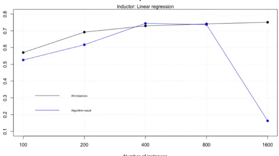
5.1.1 Model 0
As we mentioned in model explanation section, here we only use regression data, so we show results for all dataset sizes. In order to see the performance of the model, we use linear regression and validate the result using 10-fold cross validation. We compare the result obtained at the beginning with all attributes with the result obtained after remove attributes with worst position in Relief classification.
Dataset size
100 200 400 800 1600
All attributes 0.5703685 0.6921257 0.7293787 0.7410310 0.7509261
After cut 0.5258170 0.6165967 0.7441911 0.7368039 0.1628267
Table 2: Model 0 cross validation results for regression problem
We can see that model 0 increases it’s performance if dataset has more instances, but only overcome the initial result when it has 400 rows of data. We also want to note that
the worst result happens with 1600 instances, because the algorithm only returns Rel. 2
For a better look to the results we plot it in figure 9.
Figure 9: Model 0 cross validation results
5.1.2 Model 1
We have seen that model 0 is too simple and it does not present a good performance when we apply it to our dataset. In model 1 we first work with artificial regression problems to develop the base of the algorithm. In the next lines we show and describe the results of the algorithm.
For a better understanding we use plots where each point indicates which attribute is deleted before calculate the inducers’s performance. In first attempts we use linear
regression as inducers and calculate 10-fold cross validation to obtain the R-squared (R2)
value at each iteration. There are two basic parameters we want to check after algorithm execution; first is the best inducers’s result and second with how many attributes it is achieved.
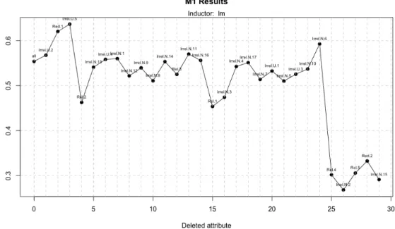
We start with a dataset of 100 instances; in figure 10 we can see that the algorithm is irregular and the Relief classification is bad since important variables are removed in the first iterations. As we can see in table 3, the algorithm needs 27 of 31 attributes to get
the best R2 result.
The performance increase when we use a dataset with 400 instances; the algorithm remove most of the irrelevant variables first and has a decrease on R-squared value when
removesRel. 5 attribute, but it isn’t good as we expect because in some final iteration it
removesIrrel. N. 5 attribute and the performance decreases a lot.
If we compare now the two last sizes, 800 and 1600 instances, we can see that the model performance is better than others, but not much. In this case it’s more interesting to take a look to the number of attributes the algorithm needs to obtain the best performance;
Figure 10: Model 1 execution with a dataset of 100 instances
in table 3 we can see that model 1 obtains its best performance with 1600 instances but it needs 12 of 31 attributes. If we take a look to 800 instances, the performance is a little bit smaller but it only needs 5 attributes.
Number of instances 100 200 400 800 1600 lm 27/31 27/31 19/31 5/31 12/31 0.63673 0.69635 0.74345 0.74678 0.75485 rf 27/31 27/31 13/31 6/31 6/31 0.53445 0.63635 0.74399 0.84605 0.87964
Table 3: Number of attributes model 1 needs to best performance in regression context Using Kendall’s correlation coefficient results (table 4) we can validate that in model 1 the best performance is achieved when the algorithm works with an 800 instances dataset. This values are similar if we use random forest because this model performs Relief classi-fication once at the beginning.
Number of instances
100 200 400 800 1600
0.2587065 0.3781095 0.4029851 0.7910448 0.6915423
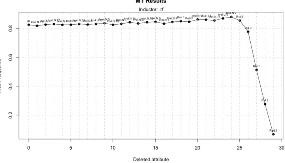
Table 4: Kendall’s correlation coefficient results for model 1 using regression dataset When using random forest as inducers, we can appreciate a better performance when we use bigger datasets (table 3). This time we securely validate that with a dataset of 1600 instances we obtain the best performance result of model 1 in regression since it
uses 6 attributes to obtain an R2 of 0.87964. Figure 11 show the execution of this best
Figure 11: Model 1 execution with a dataset of 1600 instances
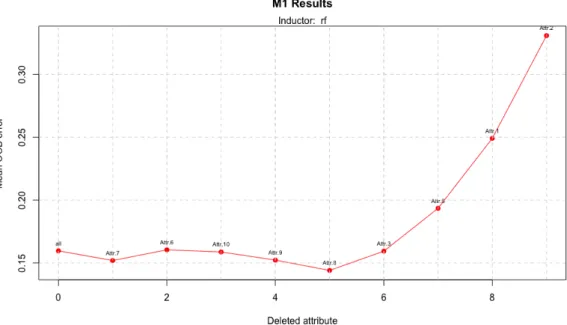
If we now take part in classification problems we can see that using both inducers, Linear Discriminant Analysis and Random Forest, the results improve while dataset size increase. As we can see in table 5, with LDA we achieve the best performance using a dataset with 800 instances but it needs 9 of 11 attributes; with 400 instances (figure 12), the accuracy is a little bit lower but it only uses 4 attributes.
Figure 12: Model 1 performance using LDA and a dataset with 400 attributes Let’s look the results if we use Random Forest. In this case the better performance is achieved with the largest dataset and it uses half of the attributes; so it is a nice
result to see. In figure 13 we can see the performance that outputs the best result in the classification context. Number of instances 100 200 400 800 1600 lm 10/11 10/11 4/11 9/11 10/11 0.79 0.79 0.825 0.8462 0.8437 rf 3/11 5/11 6/11 7/11 5/11 0.8244 0.8291 0.8475 0.86735 0.88288
Table 5: Number of attributes model 1 needs to best performance in classification context
Figure 13: Model 1 performance using RF and a dataset with 1600 attributes Kendall’s correlation coefficient confirm that in classification, the algorithm has a bet-ter performance if number of instances increase as we can see in table 6. It helps us to determine that in a classification context, use a Random Forest as inducers is the best choice.
Number of instances
100 200 400 800 1600
0.4117647 0.3529412 0.6176471 0.7058824 0.8529412
Table 6: Kendall’s correlation coefficient results for model 1 using classification dataset
5.1.3 Model 2
After an extension review of model 1, the goal of experimenting with model 2 is to see that, performing a Relief classification every time we remove the worst attribute, it increases the algorithm quality.
Like in model 1 we begin with regression artificial problems. In table 7 we can appre-ciate that, another time, when the number of instances increase the result of the inducers also increases, but this is natural for the majority of the algorithms. The performance is similar, even less to model 1 in some cases so we have to better look the number of attributes the model needs to achieve the best performance to take part in a final decision about which is the best case.
If we use Multi Linear Regression the number of attributes is lower than model one, except if we use a dataset with 800 instances where the value in model 2 is not common. With Random Forest we can appreciate a little difference if we compare to model 1 because it needs less attributes in some cases but not when we use the biggest dataset, where we obtain the best performance value.
Number of instances 100 200 400 800 1600 lm 27/31 19/31 12/31 21/31 5/31 0.6384 0.72801 0.74236 0.74778 0.75349 rf 27/31 12/31 9/31 6/31 6/31 0.51601 0.67496 0.75721 0.83847 0.87626
Table 7: Number of attributes model 2 needs to best performance in regression context In this case, we use Kendall’s correlation coefficient represented in table 8 to evaluate which inducers we use to validate model’s 2 performance. We can see that, although the inducers results are similar in both cases, the best score is achieved when we use Random
Forest and the largest dataset and this result matches with the best R2value obtained. We
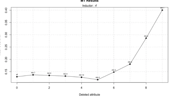
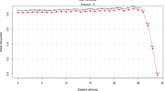
can see the best performance in figure 14, where we can see that in the final iterations the inducers result decreases a lot because the algorithm deletes the most important attributes likeRel. 3 orRel. 1.
Number of instances
100 200 400 800 1600
lm 0.1691542 0.4129353 0.800995 0.5671642 0.7064677
rf 0.1691542 0.4129353 0.800995 0.5671642 0.8208955
Table 8: Kendall’s correlation coefficient results for model 2 using regression dataset Now its time to send classification data to model 2. Linear Discriminant Analysis inducers presents the same performance as we saw in model 1, so next we explain the results obtained using Random Forest.
The improvement of the accuracy using Random Forest as inducers is small, but reaches the maximum value when we use the biggest dataset. It takes 6 of 9 attributes, while with a dataset of 200 instances it only needs 4 attributes to perform a very similar result, but the difference in the result is minimum so, another time, we need Kendall’s correlation coefficient.
If we want to use Kendall’s correlation coefficient to determine which is the best case in model 2 using classification data, we find that LDA and RF present the same value, inclusive if dataset has 400, 800 or 1600 instances. So, in this case we can determine that in a classification context with a Ranfom Forest, the algorithm works better when the
Figure 14: Model 2 performance using RF and a dataset with 1600 attributes Number of instances 100 200 400 800 1600 lm 10/11 10/11 4/11 9/11 10/11 0.79 0.79 0.825 0.8462 0.8437 rf 5/11 4/11 5/11 9/11 6/11 0.81432 0.84123 0.85598 0.87038 0.88469
Table 9: Number of attributes model 2 needs to best performance in classification context
dataset is bigger. We can see the result using a 400 instances dataset in figure 15. Number of instances
100 200 400 800 1600
lda and rf 0.6176471 0.4117647 0.7941176 0.7941176 0.7941176
Table 10: Kendall’s correlation coefficient results for model 2 using classification dataset
5.1.4 Comparison between model 1 and model 2
After reviewing model 1 and model 2 results now its time to make a comparison to deter-mine which model is better. In next lines we will compare parameters such as Kendall’s correlation coefficient, inducers best performance and time execution.
All the experiments have been done using a MacBook Pro Mid 2012 with specifications:
• Processor: 2.5 GHz Intel Core i5
Figure 15: Performance of model 2 using a dataset with 400 instances and RF
• Graphics: Intel HD Graphics 4000 1536 MB
• OS: MacOS High Sierra 10.13.2
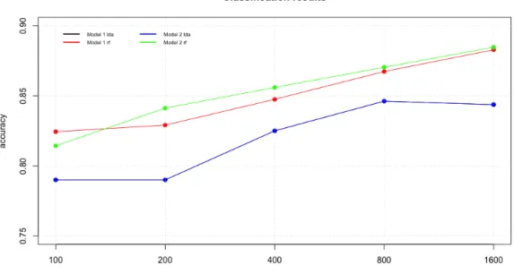
Let’s start with regression data. In figure 16 we can appreciate that Random Forest present a better performance than Linear Regression and, for a minimum difference, the best result is achieved by model 1.
Figure 16: Regression results
algorithm; that means that we need the algorithm that removes the worst attributes first. This can be checked in figure 17 where we can see that when we use Random Forest in model 2 we obtain the best result.
Figure 17: Kendall’s correlation coefficient for regression results
In the experiments related with classification if we look to the accuracy results (figure 18) we can see that model 2 achieves the better performance using Random Forest but the difference with model 1 is very small. When the inducers in LDA we can’t see a difference because both models perform the same result.
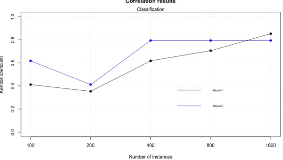
It’s time to evaluate Kendall’s correlation coefficient (figure 19) to determine which is the best model in a classification context. Another time model 2 performs the better result when using Random Forest as inducers. But what happens if we look for execution time?
Figure 19: Kendall’s correlation coefficient for classification results
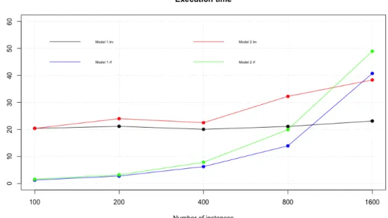
In this work the times are relatively small, but figures 20 and 21 maybe can help us to predict a time execution with a bigger dataset.
We can see that in both cases Random Forest execution is slower than Linear Regres-sion or Linear Discriminant Analysis, and all inducers present a time increment as we expected if dataset size increases.
In this point we have reviewed all models, in a regression and classification environ-ment, with different dataset size and we also review Kendall’s correlation coefficient to determine which is the best in every case. Now, its time to the user to decide which model wants to use and which inducers uses.
Figure 20: Execution time results using artificial regression data
5.2 Real data
After execute the algorithms in a controlled environment using synthetic data, its time to use real data. In this case we can’t know how good the algorithm is because we don’t know the real solution, we can only check the performance. For all real datasets we apply both models and represent in different tables the results we have obtained.
5.2.1 SkillCraft1
In terms of number of attributes, model 1 with Linean Regression (figure 22) present the best result as we can see in table 11. The difference between LM and RF in terms of performance is very small, so its not an important thing to take care of.
Model 1 Model 2
lm 5/20 19/20
0.494997 0.482394
rf 19/20 19/20
0.568231 0.568231
Table 11: SkillCraft dataset results
Figure 22: Best performance for SkillCraft dataset
5.2.2 Parkinson
With this dataset, the results are more adjusted to those predicted in the experimentation section; in table 12 we can see that the best performance, even the one that uses the least number of variables is achieved with Random Forest as inducers in model 1 (figure 23).
Model 1 Model 2 lm 19/21 19/21
0.24995 0.24933
rf 2/21 3/21
0.99783 0.98977 Table 12: Parkinson dataset results
Figure 23: Best performance for Parkinson dataset
5.2.3 Breast Cancer Wisconsin
Now we will test our algorithm in a classification problem environment. In this first case, we have obtained similar results in both models using both inducers, but Linear Discrimi-nant Analysis performs a better accuracy using less attributes than Random Forest. This performance is represented in figure 24.
Model 1 Model 2
lda 10/11 5/11
0.9628 0.9642
rf 9/11 10/11 0.9703 0.9693
Table 13: Breast cancer Wisconsin dataset results
5.2.4 Ionosphere
This dataset is the largest in terms of attributes. If we look at table 14, Random Forest uses less attributes to achieve the best inducers performance in both models; if we discard
Figure 24: Best performance for Breast Cancer Wisconsin dataset
LDA as inducers for this specific example, we can conclude that Model 1 is better than Model 2 since it uses 18 of 34 attributes and it obtains a little but better score.
To compare both models we plot each best performance in figures 25 and 26.
Model 1 Model 2
lda 25/34 28/34
0.87142 0.8687
rf 18/34 20/34 0.9419 0.9397 Table 14: Ionosphere dataset results
Figure 25: Best performance for Ionosphere dataset
Figure 26: Best performance for Ionosphere dataset using Model 2
5.3 A comparison with filter and wrapper methods
Once we develop and evaluate our models its time to compare it with some other feature selection methods.
In next tables we present the data we have obtained performing a feature selection with acorrelation filter, that finds attribute subset using correlation and entropy measures for continuous and discrete data, and a wrapper method using Linear Regression, both with
synthetic regression datasets we created in section 4.
These data has to be compared with the experiments we did in previous subsections. The only problem is that we don’t know which attributes is removed at each iteration so we don’t calculate Kendall’s correlation coefficient; correlation filter gives us the best attributes and the wrapper filter checks for each subset but we can’t extract a vector of removed attributes. In conclusions we will define what happens and what we expect with these data.
Dataset size Num. Attr. Best R2 Execution time [s]
100 4/31 0.69668 0.83124
200 4/31 0.72956 0.88516
400 4/31 0.74339 0.71084
800 4/31 0.74229 0.73792
1600 4/31 0.75249 0.77093
Table 15: Correlation filter results
Dataset size Num. Attr. Best R2 Execution time [s]
100 6/31 0.75075 1.43315
200 7/31 0.73853 1.68128
400 11/31 0.74691 1.81038
800 7/31 0.74820 3.14481
1600 11/31 0.75432 4.86907 Table 16: Wrapper filter results
6
Conclusions
This work has presented various models to perform feature selection. The slightly differ-ence from existing approach is that it uses feature weighting algorithms to improve the performance instead of pure feature selection algorithms.
Our main goal was to develop a new feature section algorithm with iterative feature weighting methods. Our idea was that every model we develop increases the previous one in terms of performance.
In the experimental section we can see that using artificial or synthetic data can help us to work in a controlled environment in order to test and validate the work. If we take a look to model 1 experiments, we can see that we achieved the best results when the dataset size is bigger. For example, in regression, using a dataset with 400 instances we
achieved an R2 of 0.74399 and the algorithms uses 13 of 31 attributes, while in a dataset
of 1600 instances we achieve an R2 of 0.87964 with only 6 of 31 attributes.
It’s important to remark that is very important to choose a good inducers. For exam-ple, in real data experiments, we can see that using Ionosphere dataset, choosing Linear Discriminant Analysis as inducers is a bad choice because we obtained an accuracy of 0.87142 using 25 of 31 attributes, while using Random Forest we obtain an accuracy of 0.9419 with 18 of 31 attributes. There are other cases, for example the experiment with
SkillCraft dataset. Here we obtain a better R2 with Random Forest, but the model uses
19 of 20 attributes. Using Linear Regression we obtained a slightly smaller R2 but it only
uses 5 of 30 attributes.
We also use Kendall’s correlation coefficient to evaluate how well a model classifies
the attributes. In regression, the best result is obtained using model 2 and Random
Forest as inducers. In classification, the best result is obtained using model 1 and Linear Discriminant analysis. The main conclusions we can extract after this work, taking into account the Kendall’s correlation coefficient, is that model 1 works better in a classification environment where we use the original Relief algorithm and model 2 work better in a regression environment.
If we take a look to the last experiment with a correlation filter and a wrapper filter, we could see that our models are only better in one case, when the dataset is the biggest and we use Random Forest as inducer. Despite this, we can conclude that our models
are not good as we expect because we gain in terms of R2 to other ones by a very little
difference and the time execution is much bigger.
I would like to comment that the hypothesis we propose in the beginning, where we said model 2 is an improvement of model 1, is not achieved as we expected because we can’t see a bigger qualitative leap. There are a lot of parameters that can be chosen by the user, depends on the parameters that are most important to him. Sometimes can be more important the number of attributes, and that means obtain a worst performance result; or sometimes can be more important the time execution.
6.1 Future work
Future work could include try another algorithm for Feature Weighting such as Simba that uses the attribute importance to calculate the distance between instances in order to perform the classification. To increase the experimental section, it can be useful to vary the sample size in datasets or increase the number of attributes. As we could see, Random Forest works very well as inducer, so another option could be tune the algorithm to increase the performance.
In synthetic datasets we worked with relevant, redundant and irrelevant features. It would be interesting to introduce corrupt data with missing values to see how the algorithm deals with it.
References
[Aha und Bankert 1996] Aha, David W. ; Bankert, Richard L.: A comparative
evaluation of sequential feature selection algorithms. (1996), S. 199–206
[Doak 1992] Doak, Justin: An Evaluation of Feature Selection Methodsand Their
Application to Computer Security. (1992)
[James u. a. 2014] James, Gareth ; Witten, Daniela ; Hastie, Trevor ; Tibshirani,
Robert: An Introduction to Statistical Learning: With Applications in R. Springer
Publishing Company, Incorporated, 2014. – ISBN 1461471370, 9781461471370
[Kira und Rendell 1992b] Kira, Kenji ; Rendell, Larry A.: A practical approach to
feature selection. In: Sleeman, D. (Hrsg.) ; Edwards, P. (Hrsg.): Machine Larning:
Proceedings of International Conference (ICML’92). Morgan Kaufmann, 1992b, S. 249– 256
[Kononenko 1994] Kononenko, Igor: Estimating attributes: analysis and extensions
of Relief. In: Raedt, L. D. (Hrsg.) ; Bergadano, F. (Hrsg.): Machine Learning:
ECML-94. Springer Verlag, 1994, S. 171–182
[Kuhn 2017] Kuhn, Max: Classification and Regression Training. : , 2017. – URL
https://github.com/topepo/caret/. – Version 6.0-78
[Leisch und Dimitriadou 2010] Leisch, Friedrich ; Dimitriadou, Evgenia: mlbench:
Machine Learning Benchmark Problems. : , 2010. – R package version 2.1-1
[Liaw und Wiener. 2015] Liaw, Andy ; Wiener., Matthew: Breiman and Cutler’s
Random Forests for Classification and Regression. : , 2015. – URL https://www. stat.berkeley.edu/~breiman/RandomForests/. – Version 4.6-12
[Mark B. und C. 2013] Mark B., Andrew H. ;C., Bill: SkillCraft1 Master Table Dataset
Data Set. 2013. – URL http://archive.ics.uci.edu/ml/datasets/skillcraft1+ master+table+dataset#
[Marko Robnik-Sikonja 2017] Marko Robnik-Sikonja, Petr S.: Classification,
Re-gression and Feature Evaluation. : , 2017. – URL https://CRAN.R-project.org/ package=CORElearn. – Version 1.51.2
[Ripley 2017] Ripley, Brian: Support Functions and Datasets for Venables and Ripley’s
MASS. : , 2017. – URL http://www.stats.ox.ac.uk/pub/MASS4/. – Version 7.3-48
[Robnik-Sikonja und Kononenko 1997] Robnik-Sikonja, Marko ; Kononenko, Igor:
An adaptation of Relief for attribute estimation in regression. In: Fisher, D. H. (Hrsg.):
Machine Learning: Proceedings of the Fourteenth International Conference (ICML’97). Morgan Kaufmann, 1997, S. 296–304
[Robnik-Sikonja und Kononenko 2003] Robnik-Sikonja, Marko ; Kononenko, Igor:
Theoretical and Empirical Analysis of ReliefF and RReliefF. In: Machine Learning 53
(2003), S. 23–69
[Sigillito 1989] Sigillito, Vince: Ionosphere. 1989. – URL https://archive.ics.
[T. und L. 2009] T., Athanasios ;L., Max: Oxford Parkinson’s Disease Telemonitoring Dataset. 2009. – URL https://archive.ics.uci.edu/ml/datasets/Parkinsons+ Telemonitoring
[Team 2008] Team, R Development C.: R: A Language and Environment for Statistical
Computing. Vienna, Austria: R Foundation for Statistical Computing (Veranst.), 2008.
– URLhttp://www.R-project.org. – ISBN 3-900051-07-0
[Wolberg 1995] Wolberg, Dr. William H.: Breast Cancer Wisconsin
(Diagnos-tic). 1995. – URL https://archive.ics.uci.edu/ml/datasets/Breast+Cancer+ Wisconsin+(Diagnostic)
Appendix
Appendix A
Model 2
model2 <− f u n c t i o n(data, i n d u c e r s , d a t a t y p e ){ s t a r t t i m e <− Sys .t i m e( ) s e t. s e e d ( 2 4 ) n <− n c o l(d a t a) n p l o t <− n # R e g r e s s i o n Problem i f (c l a s s(d a t a[ , n ] ) == ” numeric ” | | c l a s s(d a t a[ , n ] ) == ” i n t e g e r ”) { p r i n t(” R e g r e s s i o n ”) # R e l i e f l i b r a r y( CORElearn ) f o r m u l a <− a s.f o r m u l a(p a s t e(names(d a t a) [ n ] , ”˜ . ”) ) r e s u l t <− a t t r E v a l ( n , data, e s t i m a t o r=” R R e l i e f F e q u a l K ”, R e l i e f I t e r a t i o n s =1000) r e s <− a s.d a t a.frame(t( r e s u l t ) ) s o r t.d a t a <− d a t a[c(names(s o r t( r e s , d e c r e a s i n g = TRUE) ) , names(d a t a) [ n p l o t ] ) ] r e l i e f .names <− c o l n a m e s(s o r t( r e s , d e c r e a s i n g = FALSE) ) i n d u c e r s . r e s u l t <− r e p(NA, n−1) d a t a.names <− r e p(NA, n−1) # L i n e a r r e g r e s s i o n i f ( i n d u c e r s == ”lm”) { p r i n t(” L i n e a r R e g r e s s i o n ”) # C r o s s v a l i d a t i o n l i b r a r y( c a r e t ) t r a i n c o n t r o l <− t r a i n C o n t r o l ( method=” cv ”, number=10) # Complete d a t a s e tmodel <− t r a i n (f o r m u l a , d a t a=s o r t.data, t r C o n t r o l=t r a i n c o n t r o l , method=”lm”) i n d u c e r s . r e s u l t [ 1 ] <− a s.numeric(model $r e s u l t s [ 3 ] ) d a t a.names[ 1 ] <− ” a l l ” # D e l e t e one a t t r i b u t e a t a t i m e f o r ( i i n 1 : ( n−2) ) { s o r t.d a t a <− s o r t.d a t a[ , −(n−1) ]
d a t a.names[ i +1] <− r e l i e f .names[ 1 ] n <− n c o l(s o r t.d a t a) # C a l c u l a t e R e l i e f c l a s s i f i c a t i o n r e s u l t <− a t t r E v a l ( n , s o r t.data, e s t i m a t o r=” R R e l i e f F e q u a l K ”, R e l i e f I t e r a t i o n s =1000) r e s <− a s.d a t a.frame(t( r e s u l t ) ) s o r t.d a t a <− d a t a[c(names(s o r t( r e s , d e c r e a s i n g = TRUE) ) , names(d a t a) [ n p l o t ] ) ] r e l i e f .names <− c o l n a m e s(s o r t( r e s , d e c r e a s i n g = FALSE) ) # C r o s s v a l i d a t i o n
model <− t r a i n (f o r m u l a , d a t a=s o r t.data, t r C o n t r o l=t r a i n c o n t r o l , method=”lm”) i n d u c e r s . r e s u l t [ i +1] <− a s.numeric(model $r e s u l t s [ 3 ] ) p r i n t( i ) } y l a b e l <− ”R−s q u a r e d ” } # Random f o r e s t e l s e { p r i n t(”Random F o r e s t ”) l i b r a r y(” randomForest ”) # Complete d a t a s e t
r f <− randomForest (f o r m u l a , d a t a=s o r t.data, n t r e e =150 ,
p r o x i m i t y=FALSE) mR−s q u a r e d <− mean(r f $r s q ) i n d u c e r s . r e s u l t [ 1 ] <− a s.numeric(mR−s q u a r e d ) d a t a.names[ 1 ] <− ” a l l ” # D e l e t e one a t t r i b u t e a t a t i m e f o r ( i i n 1 : ( n−2) ) { s o r t.d a t a <− s o r t.d a t a[ , −(n−1) ] d a t a.names[ i +1] <− r e l i e f .names[ 1 ] n <− n c o l(s o r t.d a t a) # C a l c u l a t e R e l i e f c l a s s i f i c a t i o n r e s u l t <− a t t r E v a l ( n , s o r t.data, e s t i m a t o r=” R R e l i e f F e q u a l K ”, R e l i e f I t e r a t i o n s =1000) r e s <− a s.d a t a.frame(t( r e s u l t ) ) s o r t.d a t a <− d a t a[c(names(s o r t( r e s , d e c r e a s i n g = TRUE) ) , names(d a t a) [ n p l o t ] ) ] r e l i e f .names <− c o l n a m e s(s o r t( r e s , d e c r e a s i n g = FALSE) )
# Random F o r e s t
r f <− randomForest (f o r m u l a , d a t a=s o r t.data, n t r e e =150 ,
p r o x i m i t y=FALSE) mR−s q u a r e d <− mean(r f $r s q ) i n d u c e r s . r e s u l t [ i +1] <− a s.numeric(mR−s q u a r e d ) p r i n t( i ) } y l a b e l <− ”Mean R−s q u a r e d ” } i f (d a t a t y p e == ” a r t i f i c i a l ”) { # K e n d a l l c o r r e l a t i o n p r i n t(” K e n d a l l C o r r e l a t i o n ”) t r u t h <− c( 1 , 1 , 3 , 4 , 5 , 3 0 , 3 0 , 3 0 , 3 0 , 3 0 , 3 0 , 3 0 , 3 0 , 3 0 , 3 0 , 3 0 , 3 0 , 3 0 , 3 0 , 3 0 , 3 0 , 3 0 , 3 0 , 3 0 , 3 0 , 3 0 , 3 0 , 1 0 , 1 0 , 5 ) names( t r u t h ) <− names(d a t a[−3 1 ] ) s o l u t i o n <− s o l u t i o n <− c( 1 , 1 , 3 , 4 , 5 , 5 , 1 0 , 1 0 , 3 0 , 3 0 , 3 0 , 3 0 , 3 0 , 3 0 , 3 0 , 3 0 , 3 0 , 3 0 , 3 0 , 3 0 , 3 0 , 3 0 , 3 0 , 3 0 , 3 0 , 3 0 , 3 0 , 3 0 , 3 0 , 3 0 )
names( s o l u t i o n ) <− r e v(c(d a t a.names[ 2 : l e n g t h(d a t a.names) ] , names(s o r t.d a t a[ 1 ] ) ) ) s o l u t i o n <− s o l u t i o n [names( t r u t h ) ] m<− c b i n d( t r u t h , s o l u t i o n ) p r i n t(c o r(m, method = ” k e n d a l l ”) ) } # Add b e t t e r a t t r i b u t e t o names . f u l l
names. f u l l <− c(d a t a.names[ 2 : l e n g t h(d a t a.names) ] , r e l i e f . names)
# P r i n t which a t t r i b u t e s we need t o p e r f o r m t h e b e s t i n d u c e r s r e s u l t
a t t r i b u t e s <− names. f u l l [which.max( i n d u c e r s . r e s u l t ) :l e n g t h( names. f u l l ) ] p r i n t(p a s t e(” B e s t p e r f o r m a n c e : ”, max( i n d u c e r s . r e s u l t ) ) ) p r i n t(p a s t e(”Number o f a t t r i b u t e s needed f o r b e s t p e r f o r m a n c e : ”, l e n g t h(a t t r i b u t e s) , ” o f ”, n p l o t ) ) # P l o t r e s u l t s p l o t( 0 : ( n p l o t−2) , i n d u c e r s . r e s u l t , t y p e=” o ”, main=”M2 R e s u l t s ”, y l a b = y l a b e l , x l a b = ” D e l e t e d a t t r i b u t e ”, c o l=” r e d ”, pch =21 , bg=” r e d ”) t e x t( 0 : ( n p l o t−2) , i n d u c e r s . r e s u l t , d a t a.names, c e x = 0 . 6 , pos =3)
mtext(p a s t e(” i n d u c e r s : ”, i n d u c e r s ) , s i d e =3) g r i d( l t y =2) a b l i n e( v = 0 : ( n p l o t−2) , l t y =2 , c o l=’ l i g h t g r e y ’) } # C l a s s i f i c a t i o n Problem e l s e { p r i n t(” C l a s s i f i c a t i o n ”) # R e l i e f l i b r a r y( CORElearn ) f o r m u l a <− a s.f o r m u l a(p a s t e(names(d a t a) [ n ] , ”˜ . ”) ) r e s u l t <− a t t r E v a l (f o r m u l a , data, e s t i m a t o r=” R e l i e f ”, R e l i e f I t e r a t i o n s =1000) r e s <− a s.d a t a.frame(t( r e s u l t ) ) s o r t.d a t a <− d a t a[c(names(s o r t( r e s , d e c r e a s i n g = TRUE) ) , names(d a t a) [ n p l o t ] ) ] r e l i e f .names <− c o l n a m e s(s o r t( r e s , d e c r e a s i n g = FALSE) ) i n d u c e r s . r e s u l t <− r e p(NA, n−1) d a t a.names <− r e p(NA, n−1) i f ( i n d u c e r s == ” l d a ”) { p r i n t(” L i n e a r D i s c r i m i n a n t A n a l y s i s ”) l i b r a r y(MASS)
d a t a. l d a <− l d a (f o r m u l a , d a t a=s o r t.data, CV=TRUE)
t a b <− t a b l e(d a t a[ , n ] , d a t a. l d a$ c l a s s) a c c <− sum(d i a g(prop.t a b l e( t a b ) ) ) i n d u c e r s . r e s u l t [ 1 ] <− a s.numeric( a c c ) d a t a.names[ 1 ] <− ” a l l ” # D e l e t e one a t t r i b u t e a t a t i m e f o r ( i i n 1 : ( n−2) ) { s o r t.d a t a <− s o r t.d a t a[ , −(n−i ) ] d a t a.names[ i +1] <− r e l i e f .names[ 1 ] # C a l c u l a t e R e l i e f c l a s s i f i c a t i o n r e s u l t <− a t t r E v a l (f o r m u l a , s o r t.data, e s t i m a t o r=” R e l i e f ”, R e l i e f I t e r a t i o n s =1000) r e s <− a s.d a t a.frame(t( r e s u l t ) ) s o r t.d a t a <− d a t a[c(names(s o r t( r e s , d e c r e a s i n g = TRUE) ) , names(d a t a) [ n p l o t ] ) ] r e l i e f .names <− c o l n a m e s(s o r t( r e s , d e c r e a s i n g = FALSE) )
# LDA
d a t a. l d a <− l d a (f o r m u l a , d a t a=s o r t.data, CV=TRUE)
t a b <− t a b l e(d a t a[ , n ] , d a t a. l d a$ c l a s s) a c c <− sum(d i a g(prop.t a b l e( t a b ) ) ) i n d u c e r s . r e s u l t [ i +1] <− a s.numeric( a c c ) p r i n t( i ) } y l a b e l <− ” Accuracy ” } e l s e { p r i n t(”Random F o r e s t ”) l i b r a r y(” randomForest ”) # Complete d a t a s e t
r f <− randomForest (f o r m u l a , d a t a=s o r t.data, n t r e e =150 ,
p r o x i m i t y=FALSE) #a c c <− sum ( d i a g ( prop . t a b l e ( r f$c o n f u s i o n ) ) ) oob . e r r <− sum(r f $e r r . r a t e [ , 1 ] )/150 i n d u c e r s . r e s u l t [ 1 ] <− a s.numeric( oob . e r r ) d a t a.names[ 1 ] <− ” a l l ” # D e l e t e one a t t r i b u t e a t a t i m e f o r ( i i n 1 : ( n−2) ) { s o r t.d a t a <− s o r t.d a t a[ , −(n−i ) ] d a t a.names[ i +1] <− r e l i e f .names[ 1 ] # C a l c u l a t e R e l i e f c l a s s i f i c a t i o n r e s u l t <− a t t r E v a l (f o r m u l a , s o r t.data, e s t i m a t o r=” R e l i e f ”, R e l i e f I t e r a t i o n s =1000) r e s <− a s.d a t a.frame(t( r e s u l t ) ) s o r t.d a t a <− d a t a[c(names(s o r t( r e s , d e c r e a s i n g = TRUE) ) , names(d a t a) [ n p l o t ] ) ] r e l i e f .names <− c o l n a m e s(s o r t( r e s , d e c r e a s i n g = FALSE) ) # Random F o r e s t r f <− randomForest (f o r m u l a , d a t a = s o r t.data, n t r e e =150 , p r o x i m i t y=FALSE) #a c c <− sum ( d i a g ( prop . t a b l e ( r f$c o n f u s i o n ) ) ) oob . e r r <− sum(r f $e r r . r a t e [ , 1 ] )/150 i n d u c e r s . r e s u l t [ i +1] <− a s.numeric( oob . e r r ) p r i n t( i ) } y l a b e l <− ”OOB e r r o r ” }
i f (d a t a t y p e == ” a r t i f i c i a l ”) { # K e n d a l l c o r r e l a t i o n p r i n t(” K e n d a l l C o r r e l a t i o n ”) t r u t h <− c( 1 , 1 , 3 , 4 , 5 , 1 0 , 1 0 , 1 0 , 1 0 , 1 0 ) names( t r u t h ) <− names(d a t a[ , −11]) s o l u t i o n <− c( 1 , 1 , 3 , 4 , 5 , 1 0 , 1 0 , 1 0 , 1 0 , 1 0 )
names( s o l u t i o n ) <− r e v(c(d a t a.names[ 2 : l e n g t h(d a t a.names) ] , names(s o r t.d a t a[ 1 ] ) ) ) s o l u t i o n <− s o l u t i o n [names( t r u t h ) ] m<− c b i n d( t r u t h , s o l u t i o n ) p r i n t(c o r(m, method = ” k e n d a l l ”) ) } # Add b e t t e r a t t r i b u t e t o names . f u l l
names. f u l l <− c(d a t a.names[ 2 : l e n g t h(d a t a.names) ] , r e l i e f . names)
# P r i n t which a t t r i b u t e s we need t o p e r f o r m t h e b e s t i n d u c e r s r e s u l t
i f ( i n d u c e r s == ” r f ”) {
a t t r i b u t e s <− d a t a.names[which.min( i n d u c e r s . r e s u l t ) : l e n g t h(d a t a.names) ]
p r i n t(p a s t e(” B e s t p e r f o r m a n c e : ”, min( i n d u c e r s . r e s u l t ) ) )
}
e l s e {
a t t r i b u t e s <− d a t a.names[which.max( i n d u c e r s . r e s u l t ) : l e n g t h(d a t a.names) ] p r i n t(p a s t e(” B e s t p e r f o r m a n c e : ”, max( i n d u c e r s . r e s u l t ) ) ) } p r i n t(p a s t e(”Number o f a t t r i b u t e s needed f o r b e s t p e r f o r m a n c e : ”, l e n g t h(a t t r i b u t e s) , ” o f ”, n p l o t ) ) # P l o t r e s u l t s p r i n t(” P l o t R e s u l t s ”) p l o t( 0 : ( n p l o t−2) , i n d u c e r s . r e s u l t , t y p e=” o ”, main=”M2 R e s u l t s ”, y l a b = y l a b e l , x l a b = ” D e l e t e d a t t r i b u t e ”, c o l=” r e d ”, pch =21 , bg=” r e d ”) t e x t( 0 : ( n p l o t−2) , i n d u c e r s . r e s u l t , d a t a.names, c e x = 0 . 6 , pos =3) mtext(p a s t e(” i n d u c e r s : ”, i n d u c e r s ) , s i d e =3) g r i d( l t y =2) a b l i n e( v = 0 : ( n p l o t−2) , l t y =2 , c o l=’ l i g h t g r e y ’) } end t i m e <− Sys .t i m e( ) p r i n t(end t i m e − s t a r t t i m e)
p r i n t(”End”)
Appendix B
Model 1 regression results
Figure 27: Model 1 performance with 100 instances dataset
Figure 29: Model 1 performance with 400 instances dataset
Figure 31: Model 1 performance with 1600 instances dataset
Figure 33: Model 1 performance with 200 instances dataset
Figure 35: Model 1 performance with 800 instances dataset
Appendix C
Model 1 classification results
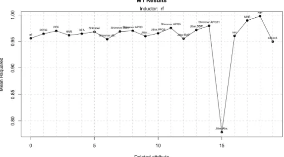
Figure 37: Model 1 performance with 100 instances dataset