Systems biology and statistical data integration of ~omics data sets

Systems biology and statistical data

integration of ~omics data sets

2

Thesis committee Promotor

Prof. Dr. R.G.F. Visser Professor of Plant Breeding Wageningen University

Co-promotor

Dr. Ir. C.A. Maliepaard

Assistant professor at the Laboratory of Plant Breeding Wageningen University

Other members

Prof. Dr. A.K. Smilde, University of Amsterdam Prof. Dr. F.A. van Eeuwijk, Wageningen University Prof. Dr. H.J. Bouwmeester, Wageningen University

Prof. Dr. Ir. M. Koornneef, Wageningen University and Max Planck Institute for Plant Breeding Research, Köln, Germany

This research was conducted under the auspices of the Graduate School Experimental Plant Sciences

Systems biology and statistical data integration

of ~omics data sets

Animesh Acharjee

Thesis

submitted in fulfilment of the requirements for the degree of doctor at Wageningen University

by the authority of the Rector Magnificus Prof. dr. M.J. Kropff,

in the presence of the

Thesis Committee appointed by the Academic Board to be defended in public

on Wednesday 12 June 2013 at 1.30 p.m. in the Aula.

4

Animesh Acharjee

Systems biology and statistical data integration of ~omics data sets 177 pages.

PhD thesis, Wageningen University, Wageningen, The Netherlands, 2013 With references, with summaries in Dutch and English

Contents

Chapter 1 6

General introduction Chapter 2 23

Comparison of regularized regression methods for metabolomics data Chapter 3 46

Data integration and network reconstruction with ~omics data using random forest regression in potato Chapter 4 66

Untargeted metabolomic quantitative trait loci (mQTL) analysis reveal a relationship between primary metabolism and potato tuber quality Chapter 5 90

Genetical genomics of quality related traits in potato tubers using proteomics Chapter 6 115

Prediction of potato quality traits from ~omics data Chapter 7 133 General discussion References 149 Summary 167 Samenvatting 170 Acknowledgements 173

About the author 175

6

Chapter 1

Potato breeding and potato quality traits

Potato (Solanum tuberosum L.) is the world’s third major food crop in terms of food

consumption, and number eight in terms of area under cultivation (FAO statistics 2008). The potato tuber is a high-energy staple food in many countries around the world.

Today’s world has a high demand of potatoes for consumption and industrial applications. To meet this demand, a continuous improvement of the potato crop by breeding is required. One of the major goals in potato breeding is high yield and an improved agronomic performance. An improvement in agronomic performance can be made in different areas such as introduction of resistance to pests and diseases, tolerance to abiotic stress factors like salinity, drought or low mineral content of soils, physiological and plant architectural traits leading to improved agricultural performance. Another area of improvement comprises quality aspects and it is an area that is likely to become ever more important in the near future. Depending on the target market, focus is shifting more towards breeding for quality. For instance, from a practical grower’s perspective, being able to produce outstanding potato quality can offer a distinctiveness that can create extra revenue (Caswell and Mojduszka 1996). The physical properties connected to quality traits, like shape, colour and size, are easily observable by consumers and are therefore major factors determining market value of a product.

The nutritional composition of potatoes is important considering the high use of this crop in diets of people around the world. Potato is rich in carbohydrate content but it also provides significant quantities of other nutrients such as proteins, minerals and vitamins (Kadam et al., 1991). For the industry (e.g. crisps) quality in terms of texture, colour, frying properties, composition in terms of starch and sugars is very important as well.

Potato skin colour, eye depth, size and shape are crucial quality aspects of fresh potatoes for consumers, as they are immediately obvious while making the purchase. Therefore, these as well as other quality traits, are being considered in breeding and genetic research (Werij 2011). In cultivated potato, the flesh colour is predominantly white or yellow. Strong cultural preference exists for either white, preferred in the US and UK, or more yellow, for instance in the Netherlands and Germany, making breeding for potato flesh colour important. Fig. 1 shows an example of white and yellow flesh colour. The yellow to orange colouring of the potato tuber flesh is caused by the presence of carotenoids (Wolters et al., 2010).

8 Figure 1: Examples of white and yellow flesh colour in potato

Tuber shape varies from long to compress/round and is measured by the ratio between length and width. Long tubers can be used for French fries while round ones are preferred for crisps. Such traits are controlled by a number of genes and highly influenced by environmental factors . Because cultivated potato is an autotetraploid species, genetic studies are complex, but there are some studies on tetraploid potato as well (D’hoop 2009). However, most genetic studies using biparental crosses are on diploid potatoes (Menendez et al., 2002; Schafer-Pregl et al., 1998). Also in this thesis, we used a diploid backcross population, indicated with ‘CxE’ where clone C (USW533.7) is a hybrid between Solanum phureja and Solanum tuberosum and clone E (77.2102.37) is the result of a cross between clone C and Solanum vernei

(Celis-Gamboa et al., 2002).

The ~omics era: data generation and plant breeding

Researchers in plant breeding are often interested in finding out how certain traits, especially quantitative traits, in plants are regulated in terms of genetic pathways, developmental processes and environmental conditions. These quantitative traits are often difficult to select for, and in some cases it is expensive or difficult to measure the phenotype. With the help of molecular markers it is possible to find statistical associations of genomic regions with the trait variation using analysis of quantitative trait loci (termed QTL analysis). However, there are certain limitations to QTL analysis: we do not directly find candidate genes due to the limited resolution of QTL mapping studies and sometimes we do not find all the genome regions involved, due to the limited power of the QTL studies. In addition, QTL analysis does not show the direct or causal relation to the trait of interest, first of all because we do not necessarily identify the causative gene(s), but also because the influence of the gene is through regulation of certain pathways. These pathways involve proteins, primary and secondary metabolites, and their influence may probably be through many processes interacting with the genes and the genetic and metabolic pathways. In

order to shed more light on these other, contributing factors, we also need to study the relationship between the traits of interest and the expression of genes and proteins, and the presence and quantitative variation of metabolites. High-throughput ~omics technologies like microarray (Brazma and Vilo 2000) mass spectrometry (e.g. LC-MS, GC-MS) (Fiehn 2002; Dunn et al., 2005) and protein chips (Aebersold and Mann 2003; Zhu et al., 2003) have gained much interest in the crop sciences. These techniques allow one to measure thousands of variables (genes, metabolites, proteins) simultaneously across populations. The data generated by these techniques - transcriptomics, metabolomics and proteomics- are often collectively denoted as ~omics data (Joyce and Palsson 2006).

Transcriptomics

Transcriptomics refers to the quantification of mRNA transcripts in a given organism, or in a particular tissue or cell type. Higher abundance of the mRNA transcripts are indicative of higher gene expression of the corresponding gene.

Common technologies for high-throughput analysis of gene expression are: cDNA microarray, oligonucleotide microarray, cDNA-AFLP (Amplified Fragment Length Polymorphism), SAGE (Serial analysis of gene expression) and RNAseq (Ozsolak and Milos 2011; Wang et al., 2009). In this Thesis we use data from cDNA microarrays to study gene expression in combination with phenotypic traits and other ~omics data sets.

Microarray

A cDNA microarray works by using the ability of a given mRNA molecule to bind specifically to, or hybridize to, its original DNA coding sequence in the form of a cDNA template spotted on an array. cDNA microarray experiments typically involve hybridising two mRNA samples, each of which has been converted into cDNA and labelled with its own fluorescent dye (usually a red fluorescent dye, Cyanine 5 (Cy5) and a green-fluorescent dye, Cyanine 3 (Cy3), on a single glass slide that has been spotted with (several thousands of) cDNA probes. Because of competitive binding between the two samples, the ratio of the red and green fluorescence intensities for each spot is indicative of the relative abundance of the corresponding cDNA in the two samples and provides information on the relative expression of the genes.

Metabolomics

Metabolomics is the comprehensive analysis in which metabolites of an organism are identified and quantified (Griffiths and Wang 2009). The components of the

10 metabolome can be viewed as the end products of gene expression that define the biochemical phenotype of a cell or tissue. Currently, some of the technologies available for analyzing a metabolome are: mass spectrometry (MS), nuclear magnetic resonance (NMR), liquid chromatography (LC), gas chromatography (GC), liquid chromatography-mass spectrometry (LC-MS), gas chromatography-mass spectrometry (GC-MS). In this thesis, we used GC-MS and LC-MS data sets which are briefly described below.

Gas Chromatography-Mass Spectrometry (GC-MS)

The GC-MS (Weckwerth 2003) approach is an analytical technique that can be used for plant metabolomics to detect mainly volatiles and primary metabolites such as organic acids and hormones. With GC-MS, first compounds are separated by GC and then transferred online to a mass spectrometer (MS) for further separation and mass detection. The GC can separate metabolites that have almost identical mass spectra (such as isomers), while MS provides fragmentation patterns that differentiate between co-eluting but chemically diverse metabolites. In this way hundreds of different compounds can be detected in parallel, although some can only be detected after deconvolution of overlapping peaks (www.systemsbiology.nl; Griffiths and Wang 2009).

One major limitation of GC is that it can only be used for volatile compounds or compounds that can be chemically transformed into volatile derivatives (derivatisation). The volatile compounds are fractionated by a gas chromatograph, which is usually coupled to a mass spectrometer. The volatile compounds that come off the GC column are not ionized and therefore first need to be ionized for (ion) mass detection and impact ionization, which is an ionization method that actually fragments each gaseous component into ion fragments. Due to the ionization method, each compound results in a specific fragmentation pattern. From the resulting mass spectra, peaks can be quantified based on their mass to charge ratios (m/z values). The fragmentation spectra of individual components are actually used to aid to the deconvolution of overlapping peaks in the total ion trace. In GC-MS each compound is thus characterized by its specific GC retention time and its specific fragmentation pattern (Griffiths and Wang 2009).

In potato breeding, metabolomic studies have progressively increased in importance as many potato tuber traits such as content and quality of starch, chipping quality, flesh colour, taste and glycoalkaloid content have been shown to be linked to a wide range of metabolites (Coffin et al., 1987; Dobson et al., 2008). GC-MS is useful for the rapid and highly sensitive detection of a large fraction of plant metabolites

covering the central pathways of primary metabolism (Roessner et al., 2000; Lisec et al., 2006). Untargeted metabolomic approaches by GC-MS have been successfully applied to assess changes in metabolites, evaluate the metabolic response to various genetic modifications (Roessner et al., 2001; Szopa et al., 2001; Davies et al., 2005), and to explore the phytochemical diversity among potato cultivars and landraces (Dobson et al., 2008; 2009).

Liquid Chromatography-Mass Spectrometry (LC-MS)

In Liquid Chromatography-Mass Spectrometry (LC-MS), analytes are separated according to their retention times on an HPLC (high performance liquid chromatography) column, and an MS-method to separate them according to their molecular masses. The LC-MS approach is similar to GC-MS (Weckwerth 2003) except that the samples are not derivatised before analysis, and an HPLC instrument is used to fractionate the samples.

Although the number and range of metabolites that can be quantified with GC-MS is impressive, an even larger number of compounds cannot be determined using GC-MS. For labile compounds, for compounds that are hard to derivatise, or hard to render volatile, LC-MS is more suitable than GC-MS. The main objective for using LC-MS analyses, also the case for this Thesis, is to detect and quantify secondary metabolites responsible for plant secondary metabolism. Due to improvements of LC-MS it is now possible to measure isoprenes, alkaloids, phenylpropanoids, glucosinolates, flavonoids, saponins and oxylipins. However, optimal extraction procedures differ for each class of compounds, and it is unlikely that a single extraction allowing accurate quantification for all the above compounds will be achievable.

Proteomics

Proteomics is the comprehensive, quantitative description of protein expression or protein-level measurements and its changes under the influence of biological (such as disease) or environmental conditions. There are various methods for generating proteomics data such as using gel electrophoresis (for example: 1-Dimensional, 2-Dimensional gel electrophoresis), or using MS based proteomics such as LC-MS, MS-MS. In this thesis, we used 2D difference gel electrophoresis (DIGE) for quantification of the protein expression.

12 Plant tissue samples are labeled prior to electrophoresis with fluorescent dyes Cy2, Cy3 or Cy5. Two samples are then mixed prior to IEF (isoelectric focusing) and resolved on the same 2D gel (Viswanathan et al., 2006). The two dyes allow a comparison of the two samples on the same gel directly. Instead of comparing two experimental samples, each sample in a larger experiment can also be compared to a reference sample containing a mixture of all samples in the experiment. This pooled standard can then be used to normalize protein abundance measurements across multiple gels in an experiment. As a consequence, each gel will contain an image with a highly similar spot pattern, simplifying and improving the confidence of inter-gel spot matching and quantification.

So far, there have been only limited potato proteomics studies, but the few that have been performed show that proteomics research might add to the identification of genes involved in certain processes (Urbany et al., 2012).

Genetical genomics

Allelic variations in the DNA sequence of genes and their regulatory regions underlie most of the phenotypic variation that has been exploited in modern crops and specifically in plant breeding (Bryan et al., 2000; Masouleh et al., 2009). Quantitative Trait Loci (QTL) (Paterson et al., 1988; Collard et al., 2005; Kearsey 1998; Kearsey and Farquhar 1998; Mackay 2001) mapping allows the identification of such genomic regions involved in quantitative traits in a segregating population (F1 of a cross between two heterozygous plants of a cross pollinator, F2, backcross, doubled haploids or recombinant inbred lines). We can consider quantified gene expression levels as molecular quantitative traits that can also be used in a QTL analysis. This approach is called ‘genetical genomics’ (Jansen and Nap 2001). More recently, metabolite and protein abundances have also been considered as molecular quantitative traits and analyzed by performing QTL analyses (Doerge 2002; Schadt et al., 2003). QTLs of gene expression profiles are denoted as expression QTLs (eQTL) (Schadt et al., 2003). By analogy, QTLs for proteomics data are called protein QTLs (pQTLs) and QTLs for metabolomics data metabolite QTLs (mQTLs) (Keurentjes et al., 2006; Kliebenstein 2007; Acharjee et al., 2011). The objective of a genetical genomics study is to identify genomic regions associated with observed variation in and between molecular quantitative traits such as gene expression. This approach can be used to identify regulatory genes that regulate other sets of genes as well as to derive information on genetic pathways and the relationship between regulatory and functional genes. Although the genetical genomics approach has successfully been applied to understand the genetic basis of ~omics data (Keurentjes

et al., 2006) there are still limitations: the mapping resolution is often not high enough to identify causal genes underlying detected QTLs (phQTLs, eQTLs, mQTLs or pQTLs) directly. However from using the different ~omics platforms, additional information will be available which can aid in identifying functional relationships, regulatory functions, DNA sequence positions and pathways.

Data integration and networks with ~omics

The rapid advances in ‘~omics’ technologies (genomics, transcriptomics, proteomics, and metabolomics) provide an opportunity to better understand the organization principles of cellular functions at different levels such as metabolite, gene or proteomic levels, but we have to link quantities of the metabolites, proteins and gene expression to a phenotype of interest. Therefore an integrative approach is needed for this (Fukushima et al., 2009). We can consider different approaches:

 Linking a phenotypic trait to a single ~omics data set (whether transcriptomics, proteomics, LC-MS or GC-MS)

 Linking a phenotypic trait to multiple ~omics data sets simultaneously  Linking two (or more) ~omics data sets to one another

Linking a phenotype to an ~omics data set

High-throughput technologies such as microarrays, LC-MS, GC-MS are commonly used to study the behaviour of genes, proteins and metabolites and typically generate large data sets. Here ‘large’ is referring to the number of genes, proteins, metabolite peaks compared to the much smaller number of samples (individuals) being tested in any given study and hence it creates a high-dimensional, multivariate data set.

In plant breeding research, phenotypic data of interest could be disease scores, growth characteristics, agronomical traits or quality traits such as flesh colour of potato, phosphate content etc. Such phenotypic data can be scored on a continuous scale, an ordinal scale or as binary scores. To link such phenotypes with ~omics data one could think of a regression approach (in case of a binary response, one could use a classification or a logistic regression approach) where the phenotypic trait is considered as a response variable and the ~omics data set as a predictor set. This makes sense as we are usually interested in the phenotypic trait as predicted from the molecular profile variation between individuals in a population. However, in such data sets the number of variables (p) is larger than the number of individuals (n) and there will be collinearity due to p>>n (Kiers and Smilde 2007) but also because of

14 high correlations among sets of variables due to common biological functions. Because of this, we cannot invert the variance-covariance matrix to estimate regression coefficients and hence traditional statistical methods such as multiple linear regression cannot be applied.

Therefore we need other methods that can be used despite the overabundance of candidate variables associated with a response variable. Traditional methods such as forward selection or forward stepwise regression could be applied but they have some limitations. In forward selection, one starts with an empty model and adds variables to the model, each time the one that gives the best improvement to the model, given the variables already present. When the improvement is no longer statistically significant, this process is stopped so that a subset of the explanatory variables is included in the model. In stepwise regression, in each step it is evaluated whether removing or adding a variable gives the best improvement of the model (Hastie et al., 2001).

The mean square error (MSE) of a regression model can be decomposed into two components: the square of the bias (difference between the estimate and the expectation of a parameter) and the variance of the parameter estimate. When there are many correlated variables in a linear regression model, their regression coefficients can become poorly determined and their estimates will exhibit high variance. A large positive regression coefficient of one variable can be canceled out by a similarly large negative coefficient of its correlated cousin. The recent statistical literature shows that approaches using regularization or penalization or shrinkage (Ghosh 2008; Hastie et al., 2001) are the most preferred in this context.

Regularization methods impose a penalty on the size of the regression coefficients; by doing so, the variance-covariance matrix can be inverted and hence we can estimate regression coefficients; those estimated coefficients will be shrunken towards zero or exactly zero due to the imposed size constraint (penalty).

Preprocessing and standardization of ~omics data sets

Preprocessing of ~omics data sets is done mainly to remove known systematic errors (other than the treatments applied or the variation we want to investigate), to improve comparability among samples. For example, background correction in a transcriptomics study is meant to remove signal that is always there, regardless of the level of gene expression. In metabolomics (LC-MS or GC-MS) data sets preprocessing steps could include baseline correction, alignment of peaks, peak detection etc. Before a statistical analysis of ~omics data, the data set is usually 10log or 2log transformed. The motivation for the log transformation is that the distribution

of expression level is typically asymmetric with a long tail at the high expression end. Many statistical tests require variables to follow a Gaussian (normal) distribution. Other advantages are that it might reduce heteroscedasticity (i.e. increasing variance with increasing mean values) and improve linearity of effects (Van den Berg et al., 2006). Depending on the statistical methods, further preprocessing may be required. One of the ways to do this, is standardization of the variables, also called autoscaling. Autoscaled variables have a mean of zero and a variance (and also standard deviation) of one, thereby if weights are induced by differences in variance or mean, this effect is taken away.

Prediction

The availability of high-throughput ~omics (transcriptomics, proteomics and metabolomics) and molecular marker data makes it possible to infer and predict direct relationships between a quantitative trait and an ~omics data set. For prediction often regression methods are used. To assess the goodness-of-fit of a regression model, R2 can be used; however, R2 does not quantify the prediction performance for new data. Therefore we are interested in assessing the quality of the model in terms of prediction; resampling methods (for example: cross-validation) can be used in order to quantify the accuracy of prediction of so-called new data (data not used to fit the model) from the actual data (data in hand used to fit the model).

In this thesis we used cross validation since an independent test set was not available. In such situations, we can apply k-fold cross validation by dividing the data set randomly into a number of folds that, together, make up the whole data set. For example, in ten-fold cross-validation (where k=10) the data set is divided into ten folds: nine tenth is then used for fitting the regression model (called the “training set”), and one tenth portion is left out and used to test the predictions (called the “test set”). All tenth parts are rotated so that they each have been the test set exactly once, so that after ten rounds every individual sample has been in the test set exactly once. In addition to this, many different random divisions into ten subsets can be generated to repeat the ten-fold cross validation, thereby avoiding that the prediction is just based on one particular division of the data set.

To evaluate the performance of regression models (Mevik et al., 2004) two parameters are used: Goodness of fit (R2) and the mean squared error of prediction (MSEP) (Mevik et al., 2004). Goodness of fit (R2) is used to describe how well the predictions fit a set of observations. It is a measure for the proportion of variability in a data set that is accounted for by the statistical model. The usual R2 from a linear regression is just a measure of goodness-of-fit of the data at hand (training data), but

16 is not usually valid for future predictions (test data). However, in the cross validation, we can estimate the R2 on the test set, as this set is used as an independent data set.

The mean squared error of prediction (MSEP) is obtained by averaging the squared prediction errors (differences between observed and predicted values) of the test samples. A lower MSEP value corresponds to a better predictive model.

Ranking of variables or variable selection

In high-dimensional ~omics data sets, we may be interested to find a relevant smaller subset of variables which, combined, are associated with the response (a phenotypic trait, usually). Procedures to find such smaller subsets are called variable selection

procedures. By doing this, it is possible to reduce the dimensionality of the data set and perhaps also to get rid of some or even many noise variables (variables which have no predictive power for the response variable) in the data set. Some of the regularization regression methods which select a single or a smaller subset of variables from a set of correlated variables are adaptive LASSO (Zou 2006) and Bayesian LASSO (Park and Casella 2008). Some of the examples of regularized regression methods which also do subset selection but select also groups of correlated variables are: LASSO (Least Absolute Sum of Squares Operator) (Tibshirani 1996), elastic net (Zou and Hastie 2005), sparse PLS regression (SPLS) (Chun and Keles 2009), group lasso (Yuan and Lin 2004) and a sparse group lasso (Friedman et al., 2010).

There are also methods which do not perform variable selection, but instead use all variables in the prediction. These methods include ridge regression (Hoerl and Kennard 1970), principal component regression (PCR) (Massy 1965), partial least squares (PLS) regression (Wold 1975), and Random Forest (RF) regression (Breiman 2001).

These methods still allow ranking of the variables based on the size of the regression coefficients or other measures of variable importance such as the Gini index in Random Forest (Breiman 2001). However, they differ in the criterion and/or the function of the regression coefficients that is being penalized. For example, in lasso it is the sum of the absolute values of the regression coefficients, in ridge regression the sum of the squares of the regression coefficients, and in elastic net a combination of both. In PLS (partial least squares) and PCR (principal component regression) the reduced number of principal/PLS components imply a penalization. The regression coefficients are shrunken due to this penalization (Hastie et al., 2001).

Some of the regularization methods have only a single parameter that needs to be optimized, for example: partial least squares regression, lasso, principal components regression, ridge regression. In other methods there might be two parameters, for example the two penalty parameters in case of elastic net regression; Random Forest, and sparse partial least squares also have two parameters that need to be optimized.

Linking a phenotypic trait to multiple ~omics data sets

If we have multiple ~omics data such as transcriptomics and metabolomics (LC-MS or GC-MS); transcriptomics and proteomics; metabolomics and proteomics; or transcriptomics, metabolomics and proteomics data sets and a trait of interest, we are in a different situation than just linking each of them separately to the trait (explained in the previous section).The aim is to find relationships among these multiple different levels of regulation with a connection to a phenotype of interest, for example to relate phenotype (e.g. potato tuber flesh colour) to gene expression and

metabolite levels. Here we can consider two possibilities: fuse multiple ~omics data sets into a single data set and treat the variables as if they are from a single data matrix and regress the phenotype on the variables in the data matrix. The other one is to treat the ~omics data sets separately and regress a phenotype separately on each one, select subsets of variables for each and then evaluate the relationships among the variables selected from the different data sets.

Linking two or more ~omics data sets

When comparing multiple ~omics data sets, we are not dealing with a single response variable versus a multivariate ~omics data set, but rather two or more multivariate data sets for which we want to find relationships. In this situation we are also not predominantly interested in predicting one data set from another one (or multiple others), but we consider the relationships between the data sets in any direction (e.g. we want to find relationships between a transcriptomics data set with a proteomics data set).

Integrating two data sets from different analytical platforms can enable an improved understanding of some underlying biological mechanisms and interactions between different functional levels. The advantage of this approach is that we can get integrated results, e.g. from multiple correlated metabolites and genes together at the same time. Different attempts have been made to integrate multiple ~omics data sets from different species such as metabolomics and proteomics in Arabidopsis thaliana

18 (ICA) (Wienkoop et al., 2008), and transcriptomics and metabolomics in Arabidopsis thaliana using orthogonal partial least squares regression (O2PLS) (Bylesjo et al., 2007), and transcriptomics, metabolomics and proteomics in grapevine berry also using O2PLS (Zamboni et al., 2010). Other related statistical methods can be canonical correlation analysis (CCA) which is an exploratory statistical method to highlight correlations between two data sets acquired on the same experimental units (n) but in case of ~omics data sets, where the number of variables (p) is much larger than the number of experimental units (n), a regularized version of canonical correlation analysis (CCA) should be applied to overcome p>>n issues (González et al., 2008). A regularized CCA allowing variable selection, sparse canonical correlation analysis was developed and applied by Waaijenborg and Zwinderman 2009 to a gene-expression microarray and a data set of DNA-markers.

A two-way variant of partial least squares (PLS) regression, PLS2 (Wold 1966) is capable of handling two or more multivariate data sets for which we want to find relationships. PLS2 has been successfully applied to biological data, such as gene expression, integration of gene expression and clinical data (with bridge PLS, Gidskehaug et al., 2007). A type of PLS2 called sparse PLS2 (Lê Cao et al., 2008, 2009) was developed to simultaneously integrate and select variables using lasso penalization (Tibshirani,1996). This method was applied to two different transcriptomics platforms: cDNA and Affymetrix chips where gene expression was measured on sixty cancer cell lines with both platforms. Such methods (CCA, O2PLS, PLS2) are relevant in this thesis as one could find multiple different levels of regulation and relationships across ~omics data sets, for example: gene expression vs. proteomics data sets, gene expression vs. metabolomics (LC-MS or GC-MS) data sets.

Networks

Genes and their gene products interact with one another and with other molecules (proteins, metabolites etc.) in a regulatory web of cause and effect including different feedback loops. Gene induction or repression occurs through the action of specific proteins, which are in turn products of certain genes, but gene expression can also be affected directly by metabolites or proteins, or through gene, gene-metabolite, gene-protein, metabolite-protein or gene-protein-metabolite complexes and their interactions. Such interactions can be modeled in a cellular network (Barabási et al., 2004 and 2011; Bernardo et al., 2005; Bansal et al., 2006) where genes, metabolites and proteins can be represented as nodes in a network and the strength of their interactions as edges in the network. Such networks come in two

types: inter-level and intra-level. In the intra-level category, we focus on relationships within one particular molecular domain; for example, a network consisting only of genes is called a gene regulatory or gene co-expression network; networks containing only metabolites are denoted as metabolite networks (Lacroix et al., 2008; Terzer et al., 2009; Han 2008; Fiehn et al., 2003). Inter-level networks consist of multiple types of molecules such as expression of genes and metabolites (Nikiforova et al., 2005; Acharjee et al., 2011), gene expression and proteins (Russo et al., 2010), metabolites and proteins (Yamada et al., 2009), expression of genes, metabolites and proteins (Yuan et al., 2008), genes, metabolites, proteins and phenotypes. In Fig. 2, we show an approach of inter-level networks by integrating ~omics data with a phenotype of interest and associations among ~omics data sets. To build an inter or an intra-level network different methods can be applied: Pearson correlation, mutual information, partial correlations etc. A detailed review about the methods can be found in Markowetz and Spang 2007. In this thesis, we used Pearson correlation coefficients (in chapter 3) for building a network with genes, metabolites and a phenotypic trait.

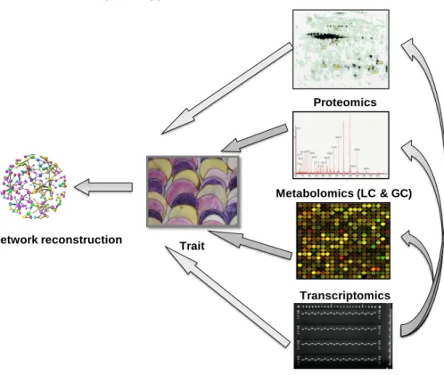
Figure 2: Integration of ~omics data sets (transcriptomics, metabolomics and proteomics) and markers with one trait (here, flesh colour) at a time to identify important metabolites, genes and proteins associated with flesh colour, followed by a correlation network analysis with a trait, genes, proteins and metabolites.

Transcriptomics Proteomics Trait Metabolomics (LC & GC) Network reconstruction Marker

20

Objectives and outline of this thesis

In this thesis we used a segregating diploid potato population (CxE) that has also been used for mapping and QTL analysis. Over the years and different research projects, much data has been accumulated: molecular marker data, phenotypic data (e.g. developmental traits, tuber quality traits), microarray data, metabolomics data (LC-MS and GC-MS) and 2D DIGE proteomics data. The current challenge and the subject of this thesis is to extract biologically meaningful associations from these data sets and relate these to phenotypes of interest, to study the methodology used to find these associations and to obtain an idea about the general reliability of the used methods and associations.

The main objective of this thesis is to link a particular phenotype to ~omics data to finally end up with a minimum set of markers (irrespective of being metabolite, transcript or protein) which can predict a quantitative trait. This objective can be subdivided into the following parts: to link phenotype to omics data, ~omics to ~omics data sets and the study of the genetics of (quantitative) traits and ~omics data sets. A further goal is to compare statistical methods suitable for ~omics data sets in terms of the prediction, correlations among variables, and ranking of genes, metabolites or proteins based for example on regression coefficients or Gini index in predictive models. To achieve this goal we considered quality traits in potato (such as tuber flesh colour, enzymatic discoloration, phosphate content, cold sweetening traits, tuber shape and starch gelatinization). We analyzed different ~omics data sets: transcriptomics, metabolomics (LC-MS & GC-MS) and proteomics data sets in the C x E potato population. These results are described in the seven chapters of this thesis.

In chapter 2 we study different regression methods to link a quantitative phenotypic trait to a metabolomics data set (the predictor data set). These regression methods are all methods that can be used in typical ~omics situations with large numbers of variables and smaller numbers of samples. We compare the methods in terms of mean square error of prediction, goodness of fit, variable selection and the ranking of the variables.

In chapter 3, we study potato tuber quality traits in relation to transcriptomics and metabolomics (LC-MS) data sets, using a Random Forest approach, and we select a subset of metabolites and transcripts that show an association with the quality traits. We construct a Pearson correlation network for two of the quality traits, flesh colour and enzymatic discoloration, with gene expression data and metabolites, leading to the integration of known and uncharacterized metabolites with genes already known

to be associated with the carotenoid biosynthesis pathway. We show that this approach enables the construction of meaningful networks with regard to metabolite pathways.

In chapter 4, we use GC-TOF-MS data sets to identify genetic factors underlying variation in primary metabolism in a mapping population. We perform a QTL analysis for starch and cold sweetening related traits and infer links between these phenotypic traits and primary metabolites. We apply Random Forest regression to find significant associations between phenotypic and metabolic traits. We confirm putative predictors in an independent collection of potato cultivars. Our results show the value of combining biochemical profiling with genetic information to identify associations between metabolites and phenotypes. This approach reveals previously unknown links between phenotypic traits and primary metabolism.

In chapter 5, we perform a proteomics analysis of potato tubers in order to obtain an insight into the relationships between protein traits and tuber quality traits such as enzymatic discoloration, starch and cold sweetening related traits. We use genetic information through QTL co-localizations and a Pearson correlation study between protein traits and quality traits. We show hot spot areas for protein QTLs consistent between data sets of two growing years (2002 and 2003). We report the first attempt for identification of protein spots of which the QTLs co-localize with quality traits. In chapter 6, we perform an integrated analysis over all the ~omics data sets. Here we study the relationship between phenotypic traits (tuber quality traits) and multiple related ~omics data sets simultaneously. We apply a genetical genomics approach to find regions of the genome explaining quantitative variation in the transcripts, metabolites and proteins predictive for quality traits. We present an approach to find a limited set of genes, metabolites and proteins for which the association to the trait is a functional relationship. First, we select subsets of genes, metabolites (LC-MS and GC-MS) and proteins showing a significant association with phenotypic traits, using Random Forest. Then variation in the expression of selected genes or in concentration of metabolites and proteins is mapped as eQTLs, mQTLs and pQTLs across the genome. Per trait, genomic regions associated with the trait are identified; in a third step, representatives of genes, metabolites and/or proteins are selected for an integrated network analysis. This integrated analysis results in a list of a minimum set of candidate genes and underlying metabolic pathways possibly linking genes, metabolites and proteins in different genomic regions underlying trait variation.

Chapter 7 provides a general discussion on all the findings. Suggestions for future approaches for the dissection of traits and ~omics data sets are given. We discuss appropriate statistical methodologies for ~omics studies in terms of prediction and

22 variable selection. We also discuss how plant breeders can use the integrated knowledge about marker and ~omics data for selecting a trait.

Chapter 2

Comparison of regularized regression methods for

metabolomics data

Animesh Acharjee1,2, Richard Finkers2,3, Richard GF Visser2,3 and Chris Maliepaard2,3

1_{Graduate School Experimental Plant Sciences, Droevendaalsesteeg 1, 6708 PB}

Wageningen, The Netherlands

2 _{Wageningen UR Plant Breeding, Wageningen University and Research Center, P.O.}

Box 386, 6700 AJ Wageningen

3_{Centre for BioSystems Genomics, PO Box 98, 6700 AB, Wageningen, The}

Netherlands

24

Abstract

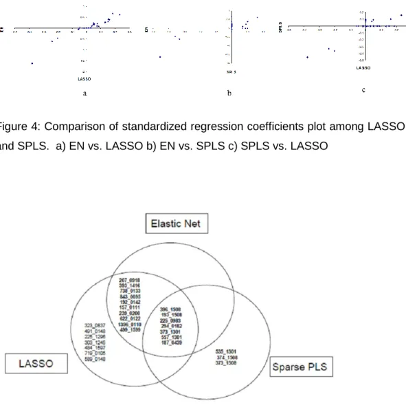
In this study, we compare methods that can be used to relate a phenotypic trait of interest to an ~omics data set, where the number or variables outnumbers by far the number of samples. We apply univariate regression and different regularized multiple regression methods: ridge regression (RR), LASSO, elastic net (EN), principal components regression (PCR), partial least squares regression (PLS), sparse partial least squares regression (SPLS), support vector regression (SVR) and Random Forest regression (RF). These regression methods were applied to a data set from a potato mapping population where we predict potato flesh colour from a metabolomics data set. We compare the methods in terms of the mean square error of prediction of the trait, goodness of fit of the models, and the selection and ranking of the metabolites. In terms of the prediction error, elastic net performed better than the other methods. Different numbers of variables are selected by the methods that allow variable selection but seven variables were in common between LASSO, EN and SPLS. SPLS performed better than EN with respect to the selection of grouped correlated variables. We developed a web application that can perform all the described methods and that includes a double cross validation for optimization of the methods and for proper estimation of the prediction error.

1 Introduction

High-throughput technologies like microarray (Brazma and Vilo 2000; Gaasterland and Bekiranov 2000) mass spectrometry (e.g., LC-MS, GC-MS) (Fiehn 2000; Dunn et al., 2005) and protein chips (Aebersold and Mann 2003; Patterson and Aebersold 2003; Zhu et al., 2003) have gained much interest in the biological domain. These techniques allow one to measure thousands of variables (genes, metabolites, proteins) simultaneously. The data generated by these techniques are often denoted as ~omics data (Joyce and Palsson 2006). These data sets are generally very large in terms of the number of variables (p) and often small in terms of the number of the biological samples (n). In statistics, this problem is often termed as the “large p and

small n problem” (p>>n). In such wide data sets there will be collinearity due to p>>n (Kiers and Smilde 2001) but also because of high correlations due to common biological functions (e.g. metabolites in the same pathway).

In many of these ~omics situations one wants to find functional relationships between a phenotypic trait of interest and the ~omics variables and often the interest would also be in selecting a smaller subset of the variables that have good prediction of the trait.

In traditional statistical methods, multiple linear regression techniques are used for prediction situations such as outlined above, but, due to the high collinearity, these methods cannot be applied. Therefore we need different approaches: penalization regression methods or machine learning methods.

We wanted to compare the different methods on real data, but we still wanted to be able to infer whether results were biologically meaningful, so we chose a trait for which a fair amount of information is already available, including a possible relationship to underlying metabolites. Therefore, we considered potato tuber flesh colour as the phenotypic trait of interest, the response in our regression, and a large metabolomics data set as the set of predictor variables. We apply a double cross validation scheme to include optimization of any hyperparameters needed in the models, and allow estimation of prediction error.

We apply different regression methods: ridge regression (RR) (Hoerl and Kennard 1970), LASSO (Tibshirani 1996), elastic net (EN) (Zou and Hastie 2005), principal component regression (PCR) (Massy 1965), partial least squares regression (PLS) (Wold 1975) sparse PLS regression (SPLS) (Chun and Keles 2009), support vector

26 regression (SVR) (Vapnik 1995) and Random Forest regression (RF) (Breiman 2001).

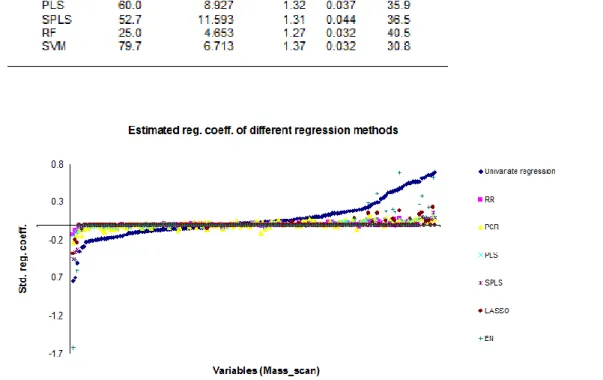
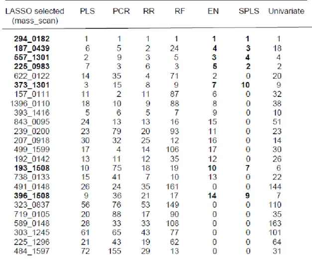
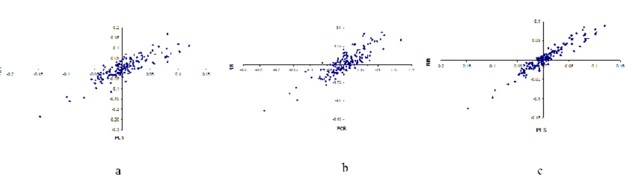
We use univariate regression as a reference and compare the results of univariate regressions with multiple regression methods. We also study the properties of these multivariate methods both from a theoretical point of view as well as their performance in practical situations in terms of the variable selection (Saeys et al., 2007) or ranking of the variables, grouping of correlated variables in variable selection (Zou and Hastie 2005), and the prediction error. Regarding the grouping of correlated variables, we are interested in finding out whether in the variable selection methods (LASSO, EN, SPLS) variables are selected as a group or not, and we also compare regression coefficients of these correlated variables.

So far in literature, comparison studies are usually focused on classification methods instead of regression methods (Hendriks et al., 2007) and data used in these studies often were transcriptomics data (Bøvelstad et al., 2007, 2009). In the context of regression, Kiers and Smilde 2001 did a comparison of various multiple regression methods on simulated data with collinear variables but their study was mainly focused on prediction and comparison of the regression coefficients when predictor variables are collinear. Menendez et al., 2012, reported comparison of stepwise linear regression, LASSO, EN and RR but did not cover other penalization methods such as SPLS, PLS, PCR, RF and SVM. We compare these methods (RR, EN, LASSO, SPLS, RF, SVM, PLS, PCR) in terms of mean square error of prediction, goodness of fit, variable selection and the ranking of the variables. In addition, we developed a web application with all the methods mentioned including the double cross validation procedure. This website can be accessed from : http://www.plantbreeding.wur.nl/omicsFusion/

2 Materials and methods 2.1 Plant material

Ninety-one individuals from a diploid mapping population of potato were used in this study. Clone C is a hybrid between Solanum phureja and Solanum tuberosum. Clone E is the result of a cross between Clone C and Solanum vernei (Celis Gamboa et al., 2003). All clones were grown in the field, Wageningen, The Netherlands in 1998. For each genotype, tubers from two plants were collected and representative samples from these tubers, of each genotype, were used for phenotypic analysis directly after harvest, and for LC-MS.

2.2 Evaluation of phenotypic traits

Many quality traits were collected for this potato population (Celis-Gamboa 2002; Celis-Gamboa et al., 2003; Werij et al., 2007). In this study we used one well-studied phenotypic trait (potato tuber flesh colour) allowing better to compare methodology and to be able to verify the results that we found. Potato tuber flesh colour was visually scored on a scale from 1 (white) to 9 (dark yellow/orange) in three repeats consisting of two plants each. Flesh colour scores were then averaged over the three repeats.

2.3 Data preprocessing

For metabolomics analysis the exact same material (potato tubers of the same genotypes) was used for Liquid chromatography–time of flight mass spectrometry (LC-QTOF MS) analysis which resulted in over 16,000 individual mass peaks. Mass peak signals below background were removed resulting in about 10,000 remaining mass peaks. The next step was to make a selection of these 10,000 peaks based on skewness of the data and all mass peaks with a skewness score below -2 and above 2 for the progeny and a score below -1 and above 1 for the parental repeats were discarded. The signal intensities of the 1,100 remaining mass peaks were then correlated to the available quality trait data of this population, in order to obtain the most interesting metabolites i.e. the metabolites linked to quality traits, P-values of these correlations were calculated using Student’s t-test. A number of 163 mass peaks with the highest significance (p<0.0005) were selected. Before analysis the metabolite data was 10logtransformed for symmetry and then autoscaled. Autoscaled variables have a mean of zero and a variance (and also standard deviation) of one, thereby giving all variables (mass scan numbers) an equal weight in the analysis. LC-MS peaks are characterized by their mass and scan number (mass_scan).

2.4 Statistical methods for regression in p >> n situations 2.4.1 Methods used

We compared the prediction, variable selection and ranking of variables. In this section, we first review the regression model in these eight methods. For all methods, values for one or more tuning parameters needed to be chosen. This was done using tenfold cross-validation, described in section of criteria for comparison of the methods.

28 Regression methods are essentially curve-fitting approaches. When there is one response variable and one predictor variable, simple linear regression consists of finding the best straight line relating the response to the predictor variable. In case of multiple predictors, a hyperplane is fitted. The usual criterion, the least squares criterion, minimizes the sum of squared distances between the observed responses and the fitted responses from the regression model (Montgomery and Peck1991). We can represent the least squares criterion as:

2 1 1

min















_

x

y



Where; y= response vector (here: flesh colour); β=regression coefficients; x=predictor variables (the log intensity values of the mass_scans from LC-MS data measured over different samples)

Here we are describing nine different regression methods which were applied to relate potato tuber flesh colour to the LC-MS data set

2.4.3 Univariate regression

Univariate regression was used as a reference. We compare the variable selection and ranking of variables in the multivariate regression methods to the results from the univariate regressions of flesh colour to each of the individual LC-MS peaks. Univariate regression with a FDR (False discovery rate) adjustment was done according to the procedure of Benjamini and Hochberg 1995.

2.4.4 Penalization or shrinkage methods

Shrinkage methods, also called penalization methods, impose a penalty on the size of the regression coefficients. The penalty term is also called a ‘regularization parameter’. We have grouped the methods according to the type of penalty applied to the regression coefficients. The mean square error (MSE) of a regression model can be decomposed into two components: the square of the bias (difference between the estimate and the expectation of a parameter) and the variance. In situations with high collinearity (p>>n), regression models usually have a very large variance and the MSE will mainly be determined by this large variance. Therefore, in such situations it can be advantageous (lower MSE) to accept some bias if it is allows us to decrease the variance by considerable amount (Hastie et al., 2001). Penalization methods impose a bias by applying a penalty to the regression coefficients.

2.4.5 Continuous penalization methods

In this category of regression methods, shrinkage factors can take any value between zero and infinity. LASSO, RR and EN belong to this category. The value of the shrinkage parameter decides the amount of penalty applied to the regression coefficients. We use tenfold cross validation (Hendriks et al., 2007) to choose the optimum penalty value; this will be discussed in detail in the section about criteria for comparison of the methods

2.4.6 Ridge regression (RR)

Ridge regression (Hoerl and Kennard 1970) shrinks the regression coefficients by imposing a penalty on the sum of squares (L2 norm) of the regression coefficients.

The left part of the term shown above is the usual least squares criterion. In the right part,



regression coefficients. The larger the value of



regression coefficients and the more they are shrunk towards zero. In ridge regression all the regressor variables stay in the model since regression coefficients do not become exactly zero (that would be equivalent to variables dropping out of the regression model). Ridge gives equal weight to absolutely correlated variables in the data set (Hastie et al., 2001).

2.4.7 LASSO

The LASSO (Least Absolute Shrinkage and Selection Operator, Tibshirani, 1996) is another regularization method but here the penalty is applied to the sum of the absolute values of the regression coefficients, the L1 norm. Mathematically, we can write this in the following way:

















_



x

y

min







Again, the left part of the term is the normal least squares criterion. The right part now is the penalized sum of the absolute values of the regression coefficients. Similar to ridge regression, the shrinkage parameter (



use tenfold cross validation for this. Penalizing the absolute values of the regression

















_



x

y

min







30 coefficients has the effect that a number of the estimated coefficients will become exactly zero which means that some regressors drop out of the regression model so that a LASSO fitted model can consist of fewer variables than the number of available regressors. In other words, LASSO can implicitly perform variable selection. The number of selected variables is upper limited by the numbers of samples (n). In case of absolutely correlated variables LASSO just selects one and ignores the rest in the group (Hastie et al., 2001).

2.4.8 Elastic net (EN)

Elastic net (Zou and Hastie 2005) is a combination of LASSO and ridge regression. It uses both a ridge penalty (penalty on the sum of the squares of the regression coefficients) and a LASSO penalty (on the sum of the absolute values of the regression coefficients):          _     













In elastic net, we optimize both penalty parameters simultaneously using tenfold cross validation. Variable selection is encouraged by the LASSO penalty (



correlated variables get similar regression coefficients. Groups of correlated variables are either in or out of the model (Zou and Hastie 2005). In contrast with LASSO, the number of selected variables is not limited by the number of individuals.

2.4.9 Discrete penalization methods:

Partial least squares (PLS) and Principal component regression (PCR) are based on latent variables or components which are linear combination of the original variables. For both methods it is essential to select the optimum numbers of latent components for prediction of the response variable. We used tenfold cross validation to choose the optimum number of latent components based on the smallest mean square error of prediction (MSEP) value. The number of latent components can only take discrete values, hence these methods are discrete penalization methods.

2.4.10 Principal component regression (PCR)

Principal component regression (Jolliffe 1982) is a combination of principal components analysis (PCA) and multiple linear regression. First, PCA is done on all original regressors and each component (latent variable) is represented by a linear combination of the original variables. The number of latent variables (components) is

chosen by tenfold cross validation and the response is regressed on the selected latent variables. These latent variables in PCA are uncorrelated. In PCR the principal components are found by maximization of the variance in the predictors; the covariance of the predictors with the response variable is not taken into account.

2.4.11 Partial least squares (PLS)

Partial least squares (PLS) (Wold 1975; Geladi and Kowlaski 1986; Hoskuldson 1988) is a method to relate a single response variable or a matrix of response variables to a matrix of regressor variables. Here, we are considering only a single trait as the response. PLS is a dimension reduction method like PCA, but it uses a different criterion: maximization of the covariance between the latent variables and the response. As a consequence, usually fewer components are required for prediction as compared to PCR. The optimum number of latent components is chosen by tenfold cross validation. Since the optimum number of latent components is a discrete number, this method is also a discrete penalization method. Like in PCR, latent variables in PLS are also uncorrelated.

2.4.12 Hybrid penalization method

In this section, we consider a method in which two different types of penalties (continuous and discrete)are applied simultaneously.

2.4.13 Sparse partial least square (SPLS)

SPLS (Chun and Keles 2009) is a combination of two different penalties. The continuous penalty is a LASSO penalty and discrete penalization is achieved by PLS. Variable selection is achieved by LASSO, dimension reduction by PLS. The respective hyperparameters i.e. the number of PLS components and the size of the LASSO penalty are optimized simultaneously by tenfold cross validation. As in normal PLS, each of the latent components is a linear combination of the original variables.

2.4.14 Machine learning methods

The goal of machine learning is to build a computer system that can adapt and learn from experience (Dietterich 1999). Machine learning methods can handle data which are not normally distributed whereas the methods mentioned above assume normality. Machine learning methods can also handle nonlinear relationships between response and predictor variables.

32 The support vector machine (SVM) (Vapnik 1995) was originally developed in a classification (Demiriz et al., 2001) context and maximizes predictive accuracy while avoiding overfitting(Hastie et al., 2001; Cristianini and Shawe-Taylor 2000) to the data.Two parameters such as epsilon (insensitive zone) and regularization parameter “C” are optimized (Vapnik 1995). However, the methodology can also be used in a regression model (Cristianini and Shawe-Taylor 2000). Mathematically, given the input data {(x1, y1), …., (xn,yn)}, we want to find a function which will fit the following

equation:

Where w is a weight vector and b is a constant

The goal of support vector regression (SVR) is to find a function f(x) that has at most ε deviation (Cristianini and Shawe-Taylor 2000) from the actually obtained targets (response)for all the predictors, and at the same time minimizes the distance between predicted and target values. SVR does not encourage grouping or variable selection.

2.4.16 Random Forest (RF)

A Random Forest (Breiman 2001) is a collection of unpruned decision trees (Hastie et al., 2001), usually developed for a classification purpose but this method can be applied in a regression context as well (Segal 2004). A RF model is typically made up of hundreds of decision trees. Each decision tree is built from bootstrap samples of the data set. That is, some samples will be included more than once in the bootstrap sample, and others will not appear at all. Generally, about two thirds of the samples will be included in this training dataset, and one third will be left out (called the out-of-bag samples or OOB samples). In RF regression the prediction error is calculated as the average prediction error over OOB predictions. Variable importance (Breiman 2001) can be quantified in RF regression. Variables used which decrease the prediction error obtain a higher variable importance. Two parameters have to be chosen in RF regression: the number of candidate variables (mtry) to choose from at any split in the regression trees, and the number of trees (ntree). The number of variables to choose from was optimized by cross validation. The number of trees was fixed at 500 trees.

2.5 Criteria for comparison of the methods 2.5.1 Double cross validation

,

)

(

x

wx

b

All methods above require input values for one or more hyperparameters (e.g. the number of components in PCR and PLS, the penalty parameter lambda in ridge regression and LASSO, etc.) and the values for these hyperparameters were optimized using cross validation. Using a single cross validation to estimate both the hyperparameters and the prediction error will result in an overly optimistic estimate of the error rate value (Smit et al., 2007). Hence, a double cross validation scheme was used (Stone 1974; Hendriks et al., 2007; Varma and Simon 2006). We used tenfold double cross validation (Hastie et al., 2001) for choosing optimum values for the hyperparameters and to estimate prediction error. First, tenfold cross validation is performed and one tenth portion of the data is left out for estimation of the prediction error, this portion is called the outer test set. The remaining nine tenth portions is the outer training set. Another tenfold cross validation uses nine tenth portions of the outer training data set which then are called the inner training sets and one tenth portions which are called the inner test sets. The hyperparameters are chosen which give the lowest MSEP values on the inner test data. We run this procedure 100 times, each with different tenfold divisions and in each division prediction was done and averaged over the results from 100 runs to obtain results in Table 1. The same divisions were used for all regression methods.

2.5.2 Mean squared error of prediction (MSEP)

The mean squared error of prediction (MSEP) is frequently used to assess the performance of regressions (Stallard et al.,1996; Mevik and Cederkvis 2004). MSEP of a regression can be estimated by predicting the test data set and comparing the predicted response with the observed response of the test set samples. Often, a (large enough) independent test set is not available. In such situations, the MSEP has to be estimated from the test data in cross-validation. An estimate of the MSEP is obtained by averaging the squared prediction errors of the outer test samples. Mathematically, we can write

MSEP = (1/n)





n

i 1

(yi – ypredicted)2

Where y and ypredicted are the observed and predicted response values for the i th test

sample, respectively. We calculated and compared the MSEP on outer test sets for all the regression methods to evaluate the different methods. We consider the lowest MSEP to correspond to a better predictive model.

34 Variable selection is defined as selecting subsets of variables that together have predictive power. LASSO, SPLS and EN are variable selection methods as they select a subset of the predictor variables. For the variable selection methods we investigated the numbers of variables and the identity of the variables which were selected by those methods. For the methods that do not include variable selection we can still rank the variables according to their estimated regression coefficients or variable importance measures. In case of RR, PLS, PCR, RF all the variables remain in the regression model. In case of SVM, we do not perform variable ranking or variable selection as we cannot estimate regression coefficients. We compare the ranking between these different methods and we compare the ranks in the ranking methods with the selection of variables in the variable selection methods.

2.5.4 Goodness of fit (R2)

Goodness of fit (R2) of statistical models is used to describe how well the predictions fit a set of observations. It is a measure for the proportion of variability in a data set that is accounted for by the statistical model. In our analysis, we use R2 values to compare the methods. R2 is calculated as the square of the Pearson correlation between observed and fitted values for training and test data set and is converted to a percentage. The usual R2 from a linear regression is just a measure of goodness-of-fit of the data at hand (training data), and not for future predictions (test data). We calculated R2 values both for training and for the cross-validation test data.

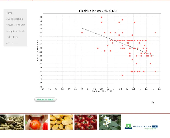
2.6 OmicsFusion web application

OmicsFusion is a web-based application written in Java EE 6 and Struts 2 and runs on a glassfish v3 application server. SQLite v3 (http://www.sqlite.org) is used as the backend database management system. Standardized excel sheets are used to upload data to OmicsFusion. The end-user can select one or several of the described methods for data analysis. A Oracle Grid Engine 6.2u5-1 cluster (http://www.oracle.com) is used to execute the R based (http://cran.r-project.org/) script in parallel. The end-user is notified by email upon completion of the analysis. Results are summarized within the web-based interface. Results which are found in this paper by analyzing metabolomics data can be found in OmicsFusion with the identifier d8933.

3 Results